Abstract—This research proposes an approach for optimizing fuzzy multiple responses using desirability function and fuzzy regression. Each response repetition is transformed into signal to noise ratio then modeled using statistical multiple regression. A trapezoidal fuzzy regression model is formulated for each response utilizing the statistical regression coefficients. The most desirable response values and the deviation function are determined for each response. Finally, four optimization models are formulated for the trapezoidal membership fuzzy numbers to obtain optimal factor level at each number. A a case study is employed for illustration. In conclusion, the proposed approach successfully dealt with inherent variability and fuzziness in multiple responses. This shall be valuable to process and product engineers for optimizing fuzzy multiple responses in manufacturing applications on the Taguchi method.
Index Terms—Desirability function, Fuzzy regression, Optimization, Taguchi method
I. INTRODUCTION
HE Taguchi [1] method utilizes a fractional factorial designs, or the so-called orthogonal arrays (OAs), to reduce the number of experiments under permissive reliability. This method has been widely accepted for obtaining robust designs in many business applications. Nevertheless, most of the published researches on the applications of the Taguchi method have been conducted to optimize a single quality response of a process or product [2, 3]. Recently, several optimization approaches have been proposed for the optimization of multiple responses [4-8].
Statistical regression has many applications [9-10], in many manufacturing processes the behavior of processes is usually vague and the observed data is irregular, hence the statistical regression models have an unnaturally wide possibility range. A fuzzy regression approach in modeling manufacturing processes, which has a high degree of fuzziness, possesses the distinct advantage of being able to
Manuscript received June, 2012; Accepted Nov., 2012. This work was supported by the University of Jordan, Amman.
A. Al-Refaie is with the Department of Industrial Engineering, University of Jordan, Amman, 11942, Jordan (e-mail: [email protected]).
I. Rawabdeh is with the Department of Industrial Engineering, University of Jordan, Amman, 11942, Jordan.
Issam Jalham is with the Department of Industrial Engineering, University of Jordan, Amman, Jordan. E-mail: [email protected]
N. Bata has received her master degree in Industrial Engineering. R. Abu-Alhaj is with the Department of Industrial Engineering, University of Jordan, Amman, 11942, Jordan.
generate models using only a small number of experimental data sets. The fuzzy regression analysis uses fuzzy numbers expressed as intervals with membership values as the regression coefficients. Fuzzy linear regression approaches have been successfully applied in many business applications [11-13].
In fact, many manufacturing processes tend to be very complex in behavior and have inherent system fuzziness; such as, fluctuation of process pressure and temperature due to environmental effects. This research, therefore, aims at optimizing multiple responses in the manufacturing application on the Taguchi method using fuzzy regression analysis.
II. THE PROPOSED OPTIMIZATION APPROACH The proposed approach for optimizing multiple responses in the Taguchi method is outlined in the following steps: Step 1: Typically, the quality response, y, is divided into three main types; involving the smaller-the-better (STB), the nominal-the-best (NTB), and the larger-the-better (LTB) response types. The Taguchi's OA conducts n experiments to investigate f factors concurrently. Let q denotes the number of responses of main concern that are measured in each experiment. To include all fuzziness in the observations values for each response, calculate the S/N ratio, ijr,at experiment i for each repetition of response j,
using an appropriate equation from the following formulas: 2
10
2 2
10 2 10
10 log ( ) for STB, 10 log ( / ) for NTB, , 10 log (1 / ) for LTB,
,
ijr
ijr
ijr ijr
ijr y
s y i j
y
r
(1)
where yiand si are the estimated average and standard deviation of yir replicates at the ith experiment. Determine the optimal factor setting for rth repetition of response j using S/N ratio. Let lfrdenotes the average of ivalues at
level l of factor f for the rth repetition. Calculate the lfr
values for all factor levels. Identify the combination of optimal factor levels for each repetition as the levels that maximize the lfrfor this factor.
Optimization of Multiple Responses in the
Taguchi Method Using Desirability Function
and Fuzzy Regression
Abbas Al-Refaie, Ibrahim Rawabdeh, Issam Jalham, Nour Bata, and Reema Abu-Alhaj
Step 2: Letjrdenotes the S/N ratio for rth repetition of response j. Obtain the multiple linear regressionsjrfor all factor level combinations using the values of ijr. That is,
2 0
1 1 <
,
1, 2,...,
v v
jr r fr f ffr f fgr f g
f f g f
x x x x
r k
(2)where 2
, ,
f f
x x andx xf gare the independent factor variables, and the coefficients, f , fg, ff are crisp values, and is random error observed in the response value. Then, determine the best-fit models for describing the functional relationship between the S/N ratio for response j and process factors. The fuzzy regression expressed as
2 0
1 1 g<
,
v v
j f f ff f fg f g
f f f
x x x x
j f
(3)
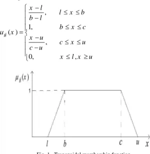
A trapezoidal fuzzy number B as shown in Fig. 1 can be defined as (l,b,c,u), where l, b, c, and u are trapezoidal limits.
The B( )x is then defined as:
, 1, ( )
,
0, ,
B
x l
l x b
b l
b x c
x
x u
c x u
c u
x l x u
(4)
Fig. 1. Trapezoidal membership function.
Let( l, b, c, u) are trapezoidal fuzzy coefficients. Obtain l, b, c
and u
as follows: m
1 k
l m
b m
c m
u m
Average( ,..., )
s
s
s
s
(5)
where s is standard deviation of (1,...,k), and is
a positive constant 0 1, chosen by an expert depending on experience about the repetitiveness of the
proposed data. For instance a large means that the expert has a poor opinion about their repetitiveness.
Step 3: Let j(xq)be jth response value by substituting the optimal fuzzy factor levels of qth response. Calculate the
( )
j xq
or all xqvalues. Provide the "most desirable"
response values for all response types using
min min
min max
max min
max 0,
( )
( ( )) , ( )
1,
j
j
j j j
j X
d X X
(6)
Let Uj and Lj denote the upper and lower limit for the desirability functions, respectively. Calculate Uj and Lj as follows
*
( ( )) , 1,...,
j j j j
U d X j q
(7)
* *
1
( ( )),..., ( ( )) , 1,...,
j j j j j q
L Min d X d X j q
(8) Step 4: Let Dj( )x denotes the deviation function to be minimized then calculate the Dj( )x using (9).
( ) ( )
( ) , 1,...,
(1 )
u c
j j
j
x x
D x j q
(9)
Then, calculate the followings
*
( )
j j j
P D x
(10)
( 1),..., ( q) ,
1,...,j j j
Q Max D x D x j q
(11) Step 5: Formulate the final model as follows
1
1
( ), ..., ( ) , 1, ...,
( ), ..., ( ) , 1, ...,
.
[Factor Levels] j
j
M ax d x d x j q M in D x D x j q s t
x
(12)
Equation (12) is converted to single objective by introducing two functionsSj( )x andTj( )x . Let
( ) ( l( ), b( ), c( ), u( ))
j j j j j
S x S x S x S x S x
(13) and
( ) ( l( ), b( ), c( ), u( ))
j j j j j
T x T x T x T x T x
whereSj( )x and Tj( )x indicate the degrees of satisfaction from desirability and robustness, respectively. Then, estimateSj( )x and Tj( )x as follows:
0, ( )
( )
( ) , ( )
1, ( )
j j
j j
j j j j
j j
j j
d x L d x L
S x L d x U U L
d x U
(15)
and
1, ( )
( )
( ) , ( )
0, ( )
j j
j j
j j j j
j j
j j
D x P Q D x
T x P D x Q
Q P
D x Q
(16)
Consequently, the objective is to maximize Sj( )x and
( )
j
T x . That is,
( ) 1, ...,
( ) 1, ...,
.
[Factor Levels]
j
j
M ax S x j q
M ax T x j q
s t x
(17)
Zimmerman Max-Min operator will be applied to convert the two-objective model to a single objective, which maximizes the minimum degree of satisfaction [14]. Let
( )
j
Min S X S
(18) and
( )
j
Min T X T
(19) Then, the final model is formulated as:
( ) ( )
M ax S X
M ax T X
(20)
Subject to: ( )
, then ( ) ( ) ,
1, ...,
j j
j j j j
j j
d X L
S d X S U L L
U L
j q
( )
, then ( ) ( ) ,
1,...,
j j
j j j j
j j
Q D X
T D X T Q P Q
Q P
j q
[Factor Levels]
x
Finally, let w1 and w2 indicate the important weights for desirability and robustness expressed by user based on cost, quality loss, and warranty. The final model with only
one objective is transformed to
1 2
1 2
.
( ) ( ) , 1,...,
( ) ( ) , 1,...,
1
0 1
0 1
[Factor Levels]
j j j j
j j j j
Max w S w T s t
d X S U L L j q
D x T Q P Q j q
w w
S T X
(21)
Solve the models l, b, c, and u to determine the values of factor fuzzy levels.
III. ILLUSTRATIVE CASE STUDY
Chen et. al [15] investigated sputtering process of GZO films using the grey-Taguchi method. Five process factors were studied including: R.F. power, x1, sputtering pressure,
x2, deposition time, x3, substrate temperature, x4, and post-annealing temperature, x5. The deposition rate (DR, y1, LTB), electrical resistively (ER, y2, STB), and optical transmittance (OT, y3, LTB) were the main responses. Let
1
i r
,i r2 , and i r3 denote the S/N ratio for DR, ER, and OT responses at experiment i(i=1,…, 18) with r (r =1, 2) repetitions, respectively. The i r1 ,i r2 , and i r3 are calculated for each repetition using the appropriate formula in (1). The obtainedi r1 ,i r2 , and i r3 are then summarized for both repetitions in Table I. The lfrvalues in each
response repetition are calculated for all factor levels for the DR, ER, and OT responses. Table II displays the lfr values
for DR, the combination of optimal factor levels for the two repetitions are identified as
(3) (2) (2) (3) (2)
1 2 3 4 5
x x x x x . In a
similar manner, the combination of optimal factor levels for the first and second repetitions of ER are found respectively as
(3) (2) (3) (3) (3)
1 2 3 4 5
x x x x x and
(3) (2) (2) (3) (3)
1 2 3 4 5
x x x x x . Finally, the combination of optimal factor levels is
(1) (1) (1) (3) (3)
1 2 3 4 5
x x x x x for both OT repetitions. It is noticed that there is a conflict among the combinations that optimize the three responses concurrently. Moreover, there are two distinct combinations of optimal factor levels for ER repetitions. This shows the fuzziness effect on ER response. The multiple linear regression equations for 11and 12are respectively written as:
3 3
11 10.29 0.08x1 0.39x2 1.2 10 x3 2.64 10 x4
4
5 8.75 10
x
4 4
12 10.42 0.08x1 0.38x2 7.2 10 x3 4.6 10 x4
4 5 7.18 10 x
21 27.499 0.1063x1 0.016x2 0.0105x3 0.0165x4
5
0.0113x ; R-Sq (adj) = 92.4%
22 27.947 0.105x1 0.394x2 0.0109x3 0.0217x4
5
0.0112x ; R-Sq (adj) = 93.1%
Finally, the multiple linear regression equations for31 and 32
are respectively expressed as:
3 3 3
31 39.202 2.34 10 x1 0.048x2 4.75 10 x3 1.11 10 x4
4 5
5.78 10 x ; R-Sq (adj) = 84.9%
3 3 3
32 39.211 2.39 10 x1 0.058x2 4.64 10 x3 1.02 10 x4
4 5
5.53 10 x ; R-Sq (adj) = 84%
Using (5), the ( l, b, c, u)values are obtained. The trapezoidal fuzzy regression 1,2and 3 are then formulated for the three responses as follows:
1
(10.28, 10.31, 10.40, 10.44) + (0.08796, 0.0797, 0.0800, 0.08022) x1 + (0.3709, 0.3772, 0.3897, 0.396) x2 + (0.0006, 0.0008, 0.0011, 0.0013) x3 + (0.00001, 0.0008, 0.0023, 0.0031) x4 + (0.0007, 0.00074, 0.00085, 0.0009) x5
2
(-28.04, -27.88, -27.57, -27.41) + (0.1047, 0.1052, 0.1061, 0.1065) x1 + (-0.0622, 0.0713, 0.3383, 0.4718) x2 + (0.0104, 0.0105, 0.0108, 0.0109) x3 + (0.0154, 0.0172, 0.0209, 0.0227) x4 + (0.0112, 0.01121, 0.0113, 0.01132) x5 and
3
(39.1999, 39.2030, 39.2093, 39.2124) + (-0.00239, -0.00238, -0.00235, -0.00233) x1 + (-0.0603, -0.0567, -0.0496,-0.0461) x2 + (-0.0048, -0.0047, -0.00465,-0.0046)
x3 + (0.001, 0.00102, 0.00107, 0.00109) x4 + (0.00055, 0.00056, 0.000575, 0.00058) x5
From Tables III to V, the values of the combinations of optimal fuzzy factor levels for DR are given calculated as
1
x = (200, 200, 200, 200), x2= (0.67, 0.67, 0.67, 0.67), 3
x = (60, 60, 60, 60), x4= (100, 100, 100, 100), and x5=
(100, 100, 100, 100). The corresponding values of 1 are (26.5432, 26.7056, 27.0392, 27.2276). Similarly, for ER the values of the combinations of optimal fuzzy factor levels are
1
x = (200, 200, 200, 200), x2= (0.67, 0.67, 0.67, 0.67), 3
x = (53.79, 64.39, 85.61, 96.21), x4= (100, 100, 100,
100), and x5= (200, 200, 200, 200). The corresponding
values of 2 are (-2.8021, -2.1555, -0.8434,-0.2114).
Finally, the values of the combinations of optimal fuzzy factor levels for OT are *
1
x = (50, 50, 50, 50), x2= (0.13,
0.13, 0.13, 0.13), x3= (30, 30, 30, 30), x4= (100, 100,
100, 100), x5= (200, 200, 200, 200). The corresponding
values of * 3
are (39.1386, 39.1496, 39.1679, 39.1769). Assuming that the acceptable ranges of min and max for DR values are equal to (12, 12, 12) and (30, 30, 30), respectively. Similarly, the values of min and max for ER are (30, 30, 30) and (-24, -24, -24), respectively. Finally, the values of min and max for OT are determined as (38, 38, 38) and (40, 40, 40), respectively. The desirability function for each response is calculated using (6) and (7) then the following values are determined:
1 (0.8080, 0.8170, 0.8355, 0.8460),
U
1 (0.1364, 0.1443, 0.1600, 0.1684)
L
2 (0.8832, 0.9102, 0.9649, 0.9912),
U
2 (0.2200, 0.2360, 0.2691, 0.2849)
L
3 (0.5693, 0.5748, 0.5840, 0.5885),
U
3 (0.2490, 0.2650, 0.3002, 0.3167)
L
Next, the fuzzy deviation functions for DR, ER, and OT are expressed respectively as:
1 1 2 3 4
5
0.0864 + 0.00044 + 0.0126 + 0.0004 + 0.0016 + 0.0001
D x x x x
x
2 1 2 3 4
5
0.3168 + 0.0008 + 0.267 + 0.0002 + 0.0036 + 0.00004
D x x x x
x
3 1 2 3 4
5
0.0062 + 0.00004 + 0.007 + 0.0001 + 0.00004 + 0.00001
D x x x x
x
Using (10) and (11), the Pj and Qjvalues are calculated and found respectively equal to
1 (0.3768, 0.3768, 0.3768, 0.3768),
P
1 (0.3844, 0.3886, 0.3971, 0.4013)
Q
2 (1.0344,1.0366,1.0408,1.0429),
P
2 (1.0344,1.0366,1.0408,1.0429)
Q
3 (0.0181, 0.0181, 0.0181, 0.0181),
P
3 (0.0303, 0.0313, 0.0335, 0.0345)
Q
wide ranges between the lower and maximal DR and ER values, whereas a tight range is noted for OT. Excluding the fuzziness will result in misleading response values if solved by the traditional regression technique. Thus, by considering
each response repetition separately, the inherent variability in the collected data is minimized.
Model b
5 5 5
1 2 3 4 5
4 4 4
1 2 3 4 5
0.5 0.5 .
0.09384 0.00443 0.021 4.44 10 4.44 10 4.11 10 0.6727 0.1443
0.16173 0.00438 0.00297 4.375 10 7.17 10 4.67 10 0.6742 0.236
0.6015 0.0011
b b
b b b b b b
b b b b b b
Max S T s t
x x x x x S
x x x x x S
4
1 2 3 4 5
1 2 3 4 5
1 2 3 4 5
9 0.0284 0.00235 0.00051 2.8 10 0.3098 0.2650
0.0863 0.00044 0.126 0.0004 0.0016 0.0001 0.0118 0.3886
0.3168 0.0008 0.267 0.0002 0.0036 0.00004 0 1.0
b b b b b b
b b b b b b
b b b b b b
x x x x x S
x x x x x T
x x x x x T
1 2 3 4 5
1 2
1 2 3 4 5
366
0.0062 0.00004 0.007 0.0001 0.00004 0.00001 0.0132 0.0313 1
0 , 1
, , , , [Factor Levels]
b b b b b b
b b
b b b b b
x x x x x T
w w S T
X x x x x x
Model c
5 4 5
1 2 3 4 5
4 4 4
1 2 3 4 5
1
0.5 0.5
.
-0.0867 0.0045 0.022 7.22 10 1.72 10 5 10 0.6776 0.1684
-0.1419 0.0044 0.0197 4.5 10 9.46 10 4.71 10 0.7063 0.2849
0.6062 0.00117 0.02
c c
c c c c c c
c c c c c c
c
Max S T s t
x x x x x S
x x x x x S
x
4 4
2 3 4 5
1 2 3 4 5
1 2 3 4 5
31 0.0023 5.45 10 2.9 10 0.2718 0.3167
0.0864 0.00044 0.126 0.0004 0.0016 0.0001 0.0245 0.4013
0.3168 0.0008 0.267 0.0002 0.0036 0.00004 0 1.0429
0.006
c c c c c
c c c c c c
c c c c c c
x x x x S
x x x x x T
x x x x x T
1 2 3 4 5
1 2
1 2 3 4 5
2 0.00004 0.0071 0.0001 0.00004 0.00001 0.0164 0.0345
1
0 , 1
, , , , [Factor Levels]
c c c c c c
c c
c c c c c
x x x x x T
w w S T
X x x x x x
TABLE I
The S/N ratios for the repetitions of sputtering experiment Exp. i
DR ER OT
11
i
i12 i21 i22 i31 i32
1 13.064 13.442 -23.464 -23.694 38.929 38.929
2 14.964 14.964 -19.825 -19.735 38.860 38.860
3 13.979 13.804 -17.953 -17.842 38.900 38.900
4 19.645 19.370 -14.648 -14.964 39.007 39.017
5 20.906 21.062 -13.255 -12.669 38.800 38.790
6 20.000 20.000 -16.258 -16.391 38.558 38.558
7 25.977 26.107 -4.0824 -4.609 38.750 38.750
8 26.689 26.690 -5.5751 -6.021 38.308 38.319
9 26.403 26.403 -5.1055 -4.082 38.649 38.619
10 13.625 13.255 -17.266 -16.902 38.850 38.850
11 13.979 13.804 -16.777 -17.025 38.998 38.998
12 13.804 13.625 -17.842 -17.730 38.830 38.830
13 19.735 19.735 -15.707 -15.417 38.790 38.7900
14 20.906 21.289 -15.563 -15.269 38.455 38.455
15 20.588 20.668 -14.807 -15.117 38.929 38.919
16 25.801 25.753 0.000 -0.828 38.392 38.392
17 26.888 26.848 -1.584 -2.279 38.660 38.600
TABLE II
THE OPTIMAL FACTOR LEVELS FOR THE TWO REPETITIONS OF DR
Factor
(f )
Replicate r =1 Replicate r =2
Level 1 Level 2 Level 3 Level 1 Level 2 Level 3
x1 16.002 20.297 26.332 13.816 20.354 26.340
x2 19.641 20.722 20.168 19.611 20.776 20.123
x3 20.095 20.270 20.167 20.089 20.288 20.132
x4 20.027 20.248 20.256 20.146 20.179 20.185
x5 20.030 20.296 20.205 20.057 20.253 20.200
TABLE III
THE OPTIMAL FACTOR LEVELS FOR THE SPUTTERING PROCESS
Model l Model b Model c Model u
* 1
x 139.84 140.73 142.52 200
* 2
x 0.13 0.13 0.13 0.13
* 3
x 30 30 30 30
* 4
x 25 25 25 25
* 5
x 0 200 200 200
IV. CONCLUSIONS
This research proposed an optimization approach using desirability function and fuzzy regression to deal with fuzzy multiple responses. A case study from previous literature are employed for illustration. It is found that the proposed approach (1) successfully deals with inherent variability and fuzziness in multiple responses by considering trapezoidal membership for each response, (2) provides ranges for optimal solution in contrast with traditional optimization techniques, (3) deals with response repetition rather than average value of response repetitions and hence provides reliable results, and (3) considers fuzzy process factor levels rather than crisp settings, hence allows flexibility in changing factor levels that may be affected during operation by uncontrollable factors. In conclusion, the proposed approach shall provide great assistance to process engineers in minimizing deviation and obtain desirable response values in manufacturing applications on the Taguchi method.
REFERENCES
[1] G. Taguchi, “Taguchi Methods,” Research and Development Dearborn, MI: American Suppliers Institute Press, vol. 1, 1991.
[2] M. H. Li, A. Al-Refaie, and C. Y. Yang, “DMAIC approach to improve the capability of SMT solder printing process,” IEEE Transactions on Electronics Packaging Manufacturing, vol. 31, no. 2,
pp. 126-133, 2008.
[3] A. Al-Refaie, M. H. Li, and R. Fouad, “Applying DMAIC procedure to improve the performance of LGP printing process companies,”
Advances in Production Engineering and Management, vol. 6, no. 1,
pp. 45-56, 2011.
[4] A. Al-Refaie, “ Optimizing SMT performance using comparisons of efficiency between different systems technique in DEA,” IEEE Transactions on Electronics Packaging Manufacturing, vol. 32, no. 4,
pp. 256-264, 2009.
[5] A. Al-Refaie, T. H. Wu, and M. H. Li, “DEA approaches for solving the multi-response problem in Taguchi method,” Artificial Intelligent for Engineering Design, Analysis and Manufacturing, vol. 23, pp.
159-173, 2009.
[6] A. Al-Refaie, “Super-efficiency DEA approach for optimizing multiple quality characteristics in parameter design,” International Journal of Artificial Life Research, vol. 1, no. 2, pp. 58-71, 2010.
[7] A. Al-Refaie, and D. M. Al-Tahat, “Solving the multi-response problem in Taguchi method by benevolent formulation in DEA,”
Journal of Intelligent Manufacturing, vol. 22, pp. 505-421, 2011.
[8] A. Al-Refaie, M. H. Li, and K. C. Tai, “Optimizing SUS 304 wire drawing process by process by grey analysis utilizing Taguchi method,” Journal of University of Science and Technology Beijing, Mineral, Metallurgy Material, vol. 15, no. 6, pp. 714-722, 2009.
[9] Y. T. Shu, D. J. Ming, T. W. Jen, and S. W. Chun, “A robust design in
hardfacing using a plasma transfer arc,” International Journal of Advanced Manufacturing Technology, vol. 27, pp. 889–896, 2006.
[10] B. M. Gopalsamy, B. Mondal, and S. Ghosh, “Taguchi method and ANOVA: An approach for process parameters optimization of hard machining while machining hardened steel,” Journal of Scientific and Industrial Research, vol. 68, pp. 686-695, 2009.
[11] H. Tanaka, S. Uejima, and K. Asai, “Linear Regression Analysis with
Fuzzy Model,” IEEE Transactions on Systems, Man, and Cybernetics SMC, vol. 12, pp. 903–907, 1982.
[12] C. Wen, and C. Lee, “Development of a cost function for wastewater treatment systems with fuzzy regression,” Fuzzy Set System, vol. 106,
pp 143–153, 1999.
[13] S. B. Oh, W. Kim, and J. K. Lee, “An approach to causal modeling in
fuzzy environment and its application,” Fuzzy Set System, vol. 35, pp.
43–55, 1990.
[14] H. J. Zimmermann, Fuzzy Sets, Decision Making and Expert Systems.
Kluwer, Boston, 1987.
[15] C. C. Chen, C. C. Tsao, Y. C. Lin, and C. Y. Hsu, “Optimization of the sputtering process parameters of GZO films using the Grey– Taguchi method,” Ceramics International, vol. 36, pp. 979–988,