www.atmos-chem-phys.net/16/1545/2016/ doi:10.5194/acp-16-1545-2016
© Author(s) 2016. CC Attribution 3.0 License.
Observations of surface momentum exchange over the marginal ice
zone and recommendations for its parametrisation
A. D. Elvidge1,a, I. A. Renfrew1, A. I. Weiss2, I. M. Brooks3, T. A. Lachlan-Cope2, and J. C. King2
1School of Environmental Sciences, University of East Anglia, Norwich, UK 2British Antarctic Survey, Cambridge, UK
3School of Earth and Environment, University of Leeds, Leeds, UK
apresent address: Atmospheric Processes and Parametrisations, Met Office, Fitzroy Road, Exeter, UK
Correspondence to:A. D. Elvidge ([email protected])
Received: 17 August 2015 – Published in Atmos. Chem. Phys. Discuss.: 1 October 2015 Revised: 5 January 2016 – Accepted: 15 January 2016 – Published: 10 February 2016
Abstract. Comprehensive aircraft observations are used to characterise surface roughness over the Arctic marginal ice zone (MIZ) and consequently make recommendations for the parametrisation of surface momentum exchange in the MIZ. These observations were gathered in the Barents Sea and Fram Strait from two aircraft as part of the Aerosol–Cloud Coupling And Climate Interactions in the Arctic (ACCA-CIA) project. They represent a doubling of the total num-ber of such aircraft observations currently available over the Arctic MIZ. The eddy covariance method is used to derive estimates of the 10 m neutral drag coefficient (CDN10)from
turbulent wind velocity measurements, and a novel method using albedo and surface temperature is employed to derive ice fraction. Peak surface roughness is found at ice frac-tions in the range 0.6 to 0.8 (with a mean interquartile range in CDN10 of 1.25 to 2.85×10⁻³).CDN10 as a function of
ice fraction is found to be well approximated by the nega-tively skewed distribution provided by a leading parametri-sation scheme (Lüpkes et al., 2012) tailored for sea-ice drag over the MIZ in which the two constituent components of drag – skin and form drag – are separately quantified. Cur-rent parametrisation schemes used in the weather and climate models are compared with our results and the majority are found to be physically unjustified and unrepresentative. The Lüpkes et al. (2012) scheme is recommended in a compu-tationally simple form, with adjusted parameter settings. A good agreement holds for subsets of the data from different locations, despite differences in sea-ice conditions. Ice con-ditions in the Barents Sea, characterised by small, unconsoli-dated ice floes, are found to be associated with higherCDN10
values – especially at the higher ice fractions – than those of Fram Strait, where typically larger, smoother floes are ob-served. Consequently, the important influence of sea-ice mor-phology and floe size on surface roughness is recognised, and improvement in the representation of this in parametrisation schemes is suggested for future study.
1 Introduction
Sea-ice movement is determined by five separate forces: a drag force from the atmosphere, a drag force from the ocean, internal sea-ice stresses, a downhill ocean-surface slope force, and the Coriolis force (e.g. Notz, 2012). The two drag forces are associated with a surface exchange of mo-mentum across the atmosphere–ice or the ice–ocean bound-ary respectively. These exchanges impact the dynamical evo-lution of both atmosphere and ocean; here we focus on the interaction with the atmosphere only. Within the atmospheric surface layer (where the turbulent stress remains close to its surface value) the wind speed,U (z), is related to the surface stress through
U=u∗ κ
ln
z z0
−ϕ
, (1)
whereu∗ is the friction velocity,κ is the von Karman con-stant (0.4), z0 is the roughness length for velocity, and
the level at which the wind speed described by Eq. (1) be-comes 0 and represents the physical roughness of the surface (Stull, 1988). The momentum exchange (or wind stress) is then
τ =ρu2∗=ρCDU2, (2)
whereρis the density andCDis the drag coefficient for the fluid at heightz. Combining Eqs. (1) and (2) we can directly relate the drag coefficient and roughness length; for example, for neutrally stratified conditions andz=10 m,
CDN10=
u
∗
U10N 2
= κ
2
ln 10 z02
. (3)
Over a rough surface the drag has two components: a sur-face skin drag caused by friction and a form drag caused by pressure forces from the moving fluid impacting on rough-ness elements (Arya, 1973, 1975). The form drag acts on sea-ice ridges, on floe edges, on melt pond edges, and on surface undulations of all types. In other words, it is a function of the morphology of the sea ice and consequently it is strongly related to ice concentration and thickness.
To parametrise surface drag in numerical weather predic-tion, or climate or Earth system models, the above formulae are implemented to determine the surface stress for a given fluid velocity and stability1. To do thisCD, or equivalently
z0, must be prescribed and so observations of these
param-eters for different sea-ice surfaces are required. To calculate these for the atmosphere–ice boundary, for example, obser-vations of surface-layer momentum flux, wind speed, and at-mospheric stability are required. These are challenging ob-servations to make over sea ice and even more challenging over the marginal ice zone (MIZ).
Over the main sea-ice pack, with ice fraction,A, close to 1, early studies based on tower or aircraft observations of turbulent fluxes estimatedCDN10in the range∼1–4×10⁻³
for continuous sea ice, depending on the ice morphology. In a comprehensive review, Overland (1985) breaks down this range by morphology and location: for large flat floes CDN10ranges 1.2–1.9×10⁻³and a median of 1.5×10⁻³is
given (e.g. based on Banke and Smith, 1971 over the Cana-dian Arctic); for rough ice with pressure ridgesCDN10ranges
1.7–3.7×10⁻³; over first year ice in marginal seas (e.g. the
Beaufort Sea or Gulf of St Lawrence) theCDN10subjective
median values are 2.2–3.0×10⁻³. More recently, Castellani
et al. (2014) use airborne-derived laser altimeter data gath-ered between 1995 and 2011 in conjunction with a sea-ice drag parametrisation scheme to demonstrate the considerable topographic and geographic variability in CDN10 over Arc-tic pack ice, with values ranging between 1.5 and 3×10⁻³,
largely corroborating the results of earlier studies.
1Note a turning angle between the fluid and the ice surface is also required if the surface-layer Ekman spiral is not resolved (Notz, 2012; Tsamados et al., 2014).
For the MIZ, data are not so readily available. On the “in-ner MIZ”, with ice fractions of 0.8–0.9 and consisting of small and rafted floes, Overland (1985) report only a few data sets, withCDN10in the range 2.6–3.7×10⁻³; while for the “outer MIZ”, withA=0.3–0.4, the only two values provided areCDN10=2.2 and 2.8×10⁻³from MIZEX-1984 over the
Greenland Sea (Overland, 1985) and from the Antarctic MIZ using an indirect balance method (Andreas et al., 1984). Fur-ther drag measurements over the MIZ using aircraft were made by Hartman et al. (1994) and Mai et al. (1996) as part of the “REFLEX” and “REFLEX II” experiments over Fram Strait. Hartman et al. (1994) obtained 16CDN10values
with ranges ofCDN10=1.0–2.3× 10⁻³forA=0.5–0.8 and CDN10=1.1–1.6×10⁻³ forA=0.9–1.0. They found gen-erally higherCDN10values over ice fractions of 0.5–0.8. Mai
et al. (1996) found a similar range over their 85 12-km runs, withCDN in the range∼1.3×10⁻³ over open water, to a
maximum of∼2.6×10⁻³ atA=0.5–0.6, then decreasing
to about 1.8×10⁻³forA=1. Schröder et al. (2003) largely corroborate these results with their 32 runs, finding a mean CDN10of 2.6×10⁻³forA=0.5 over Fram Strait and a mean CDN10of 1.6×10⁻³forA=0.86 over the Baltic Sea. These aircraft-based MIZ drag results are compiled together in Lüp-kes and Birnbaum (2005). In short, they suggest thatCDN10
peaks over the MIZ (A≈0.5–0.6) and decreases for lower or
higher ice fractions.
Sim-ulations of the near-surface atmosphere can also be signifi-cantly affected (Rae et al., 2014).
Here we present over 200 new estimates of surface drag over the MIZ in Fram Strait and the Barents Sea from two independent research aircraft. This represents a more than doubling of theCDNestimates currently available for surface
exchange parameterisation development. Only low-level legs (mainly 30–40 m a.s.l.) are used to provide quality-controlled eddy covariance estimates of the turbulent momentum flux. We use these data to provide a validation of the leading parametrisation schemes and make recommendations for pa-rameter settings. In the next section we present a brief review of surface exchange parametrisations. Section 3 covers data and methods and Sect. 4 presents our results. In Sect. 5 rec-ommendations for the parametrisation of drag in the MIZ are made, before our conclusions in Sect. 6. Note that a summary of notation is provided at the end of the paper.
2 Parametrising surface momentum exchange over sea ice
2.1 Background
All atmospheric models require an exchange of momen-tum with the surface for accurate simulations. Over sea ice this has generally been treated rather crudely, usually with a constant drag coefficient prescribed for all sea-ice types and thicknesses (e.g. Notz, 2012; Lüpkes et al., 2013). For model grid boxes that are partially ice-covered a “mosaic method” is commonly employed, which typically calculates the flux over the ice and water surfaces separately, then aver-ages these in proportion to the surface areas (e.g. Claussen, 1990; Vihma, 1995). Unfortunately, using this approach with a constant drag coefficient doesnotrepresent momentum ex-change over the MIZ correctly. It results in a linear function ofCDN withArather than the maximum in drag at interme-diate ice concentrations supported by observations.
Both empirical and physical-based parametrisations of surface drag have recently been developed. Andreas et al. (2010) composited together all available MIZ CDN
ob-servations (primarily from Hartmann et al., 1994 and Mai et al., 1996) with the vast number of summertime sea-ice pack CDN observations from the SHEBA project (Uttal et
al., 2002) forA >0.7. They argued that summertime sea ice, replete with melt ponds and leads, was morphologically sim-ilar to the MIZ and so these data sets could be combined. Plotting CDN againstA, and ignoring various outliers, they found a maximum inCDNaroundA=0.6. They empirically fitted by eye a second-order polynomial to this data set: 103CDN=1.5+2.233A−2.333A2. (4) Here,CDNis simply a function of ice fraction (A), and other
morphological characteristics are neglected.
A series of physical-based parametrisation schemes for surface drag has also been developed based on trying to cap-ture the effect of form drag by equating sea-ice character-istics to roughness elements. The form drag is added to the skin drag to give a total surface drag, as represented in these schemes by
CDN=(1−A) CDNw+ACDNi+CDNf, (5) whereCDNwandCDNiare the neutral skin drag coefficients
over open water and continuous ice respectively, andCDNfis the neutral form drag coefficient. This approach has its basis in work by Arya (1973, 1975) that has been developed and refined – see Hanssen-Bauer and Gjessing (1988), Garbrecht et al. (1999, 2002), Birnbaum and Lüpkes (2002), Lüpkes and Birnbaum (2005), Lüpkes et al. (2012), and Lüpkes and Gryanik (2015).
Amongst the leading MIZ drag schemes currently being implemented is that set out in Lüpkes et al. (2012; referred to hereafter as L2012). This scheme has been adapted for use in the Los Alamos sea-ice model CICE (Tsamados et al., 2014; Hunke et al., 2015). It determines neutral 10-m drag coefficients (CDN10)over 3-dimensional ice floes as a func-tion of sea-ice morphological parameters: sea-ice fracfunc-tion as a minimum and, optionally, freeboard height and floe size. Lüpkes et al. (2013) illustrate the substantial impact such a parametrisation has onCDN for summertime Arctic sea ice in contrast to the constant exchange coefficient approach that is currently standard in climate models.
2.2 Derivation of form drag
As a result of its sensitivity to sea-ice morphology, represent-ing the form drag component ofCDN in a parametrisation scheme is a complex procedure. Its derivation in the L2012 scheme is best approached by considering a domain, of area St, containingN identical ice floes of cross-wind lengthDi
and freeboard heighthf. If the area fraction of ice within the
domain is given byA,
St=csN D 2 i
A , (6)
wherecsrelates the deviation of the mean floe area from that
of a square (so that cs=1 for a square and, for example,
cs=π r 2
4r2 = π
4 for a circle). The total form drag acting on the
frontal areas of ice floes within the domain is provided by
fd=N cwSc2Di
hf
Z
z0w
ρ[U (z)]2
2 dz. (7)
Here,cwis the fraction of the available force which
effec-tively acts on each floe (Garbrecht et al., 1999);Scis the
towards 1 for large distances;z0wis the mean local roughness length over open water; andU (z)is the upstream wind speed. Recall from Eq. (1) thatU (z)increases logarithmically with height, so the 10 m neutral wind speed is
UN10=(u∗/κ)ln(10/z0w) . (8)
Noting that the surface wind stress due to form drag is simply the frontal force per unit area τd=fd/St,CDNf can be evaluated at the 10 m height according to Eqs. (3) and (8) as follows:
CDN10f= τd
ρUN102 =
fd/ St
ρ (u∗/κ)2ln2(10/z0w). (9) Equations (6) and (7) are inserted into Eq. (9), and the in-tegral in Eq. (7) is solved with the aid of Eq. (8) to yield
CDN10f=Ahf DiS
2 c
ce
2
"
ln(hf/z0w)−12+1−2z0w/hf
ln2(10/z 0w)
#
, (10)
where the effective resistance coefficientce=cw/cs. Finally,
following the removal of insignificant terms in the above (re-sulting in a deviation typically less than 1 % according to L2012), we obtain
CDN10f=Ahf DiS
2 c
ce
2 "
ln2(hf/z0w) ln2(10/z0w) #
. (11)
2.3 The L2012 parametrisation: equation summary The overall drag coefficient is the sum of the skin and form drag components, so substituting Eq. (1) into Eq. (5): CDN10=(1−A) CDN10w+ACDN10i
+Ahf DiS
2 c
ce
2 "
ln2(hf/z0w) ln2(10/z0w) #
. (12)
Note that our Eqs. (11) and (12) are identical to L2012 Eqs. (51) and (22). L2012 definesCDN10wandCDN10ias skin drag terms. However, this assumes there is no form drag over open water or continuous sea ice, since the form drag contri-bution given by Eq. (11) only accounts for form drag on ice floe edges. In reality, additional form drag can be produced in the ocean due to waves, and over ice due to ridging and other roughness features caused by deformation and melt. Conse-quently,CDN10wandCDN10iare better expressed as the total
(skinandform) drag over open water and continuous sea ice, respectively. The former is provided by
CDN10w=κ2ln−2(10/z0w), (13)
using Eq. (3). Note that z0w is usually provided in models
as a function of the surface stress on the sea surface and the gravitational restoring force via a modified Charnock relation
z0w=αu
2 ∗
g +b υ
u∗, (14)
whereαis the Charnock constant,bis the smooth-flow con-stant, andυis the dynamic viscosity of air (e.g. Fairall et al., 2003). L2012 setα=0.018 and b=0. It is more common to include the smooth-flow term, usually withb=0.11, so that there is some momentum exchange at low wind speeds (e.g. Renfrew et al., 2002; Fairall et al., 2003). The first term leads to an increase in roughness, and hence drag coefficient, as the wind speed increases. This increase is related to wave-induced roughness and is now reasonably well constrained for low to moderate wind speeds, but there is some uncer-tainty at higher wind speeds (Fairall et al., 2003; Petersen and Renfrew 2009; Cook and Renfrew 2015). Various values for the Charnock “constant” are used, typically between 0.011 and 0.018. In the Fairall et al. (2003) review they suggest thatαshould linearly increase from 0.011 to 0.018 (between UN10=10–18 m s−1), although they note some uncertainty
inαforUN10above 10 m s−1.
For the drag over continuous ice, L2012 recommend CDN10i=1.6×10⁻³. This is consistent with the range of values for the total drag over large flat floes, CDN=1.2– 1.9×10⁻³, given in Overland (1985) making the assumption
that the form drag over flat floes is negligible. This choice for CDN10iis also typical of the values commonly set in
numeri-cal models (Lüpkes et al., 2013).
L2012 provides three formulations for the sheltering func-tion,Sc. The form chosen for the CICE model (Tsamados et
al., 2014) is
Sc=
1−exp
−sDw hf
, (15)
wheresis a dimensionless constant and the distance between floes,Dw=Di
1−√A/√A(after Lüpkes and Birnbaum, 2005). Equations (12)–(15) together with the recommended parameters set out in Table 1 establish the parametrisation ofCDN10as a function ofA,hf,Di, andu∗. In many mod-els, however, freeboard heights and floe lengths are not avail-able. In this instance, L2012 provides further simplifications to present bothhfandDiin terms ofA:
hf=hmaxA+hmin(1−A), (16)
Di=Dmin
A
∗
A∗−A β
, (17)
where
A∗= 1
1−(Dmin/Dmax)1/β (18)
Table 1. Parameter settings for the form drag component of the L2012 scheme (Lüpkes et al., 2012): as recommended in L2012, as used in CICE (Tsamados et al., 2014), and as recommended here (E2016A and E2016B).
ce s Dmin Dmax hmin hmax β
L2012 0.3 0.5 8 m 300 m 0.286 m 0.534 m 1 CICE 0.2 0.18 8 m 300 m 0.286 m 0.534 m 1 E2016A 0.17 0.5 8 m 300 m 0.286 m 0.534 m 1 E2016B 0.1 0.5 8 m 300 m 0.286 m 0.534 m 0.2
3 Data collection and methodology
3.1 Data collection and aircraft instrumentation The data used for this study are from research flights over the Arctic MIZ using two aircraft: a DHC6 Twin Otter oper-ated by the British Antarctic Survey and equipped with the Meteorological Airborne Science INstrumentation (MASIN) and the UK Facility for Airborne Atmospheric Measurement (FAAM) BAe-146. Data from eight flights are used here, conducted between 21 and 31 March 2013 as part of the first ACCACIA (Aerosol–Cloud Coupling and Climate In-teractions in the Arctic) field campaign. The relevant flight legs are located both to the northwest of Svalbard over Fram Strait and southeast of Svalbard in the Barents Sea (Fig. 1). Wintertime sea ice in the Barents Sea is relatively thin and, owing to a cool southward-flowing surface ocean current and cyclone activity in the region, tends to extend further south than in Fram Strait where the warm North Atlantic Current has a greater influence (Johannessen and Foster, 1978; Sor-teberg and Kvingedal, 2006).
To estimate surface momentum flux from the aircraft re-quires high-frequency measurements of wind velocity and altitude, along with an estimate of atmospheric stability. To measure 3-D winds the MASIN Twin Otter uses a nine-port Best Aircraft Turbulence (BAT) probe (Garman et al., 2006) mounted on the end of a boom above the cockpit and extend-ing forward of the aircraft’s nose; while the BAE146 uses a five-port radome probe on the nose of the aircraft. To mea-sure altitude at low levels both aircraft use radar altimeters. To measure air temperatures both aircraft use Rosemount sensors (non-deiced and deiced), while to measure sea sur-face temperature (SST) both aircraft use Heimann infrared thermometers. For the calculation of albedo (used to derive estimates of sea-ice concentration), both aircraft use Eppley PSP pyranometers to measure shortwave radiation. Further details about the instrumentation – calibration, sampling rate, resolution, and accuracy – can be found in King et al. (2008) and Fiedler et al. (2010) for the MASIN Twin Otter, and in Renfrew et al. (2008) and Petersen and Renfrew (2009) for turbulence measurements on the BAE146. For brevity these details are not reproduced here.
In general, the aircraft measurements are processed iden-tically. One exception is in the calibration of SST. Here the
Figure 1.Map of Svalbard (landmass in grey) and the surround-ing ocean and sea ice. The blue–white shadsurround-ing conveys the mean sea-ice fraction from the satellite-derived Operational Sea Surface and Sea Ice Analysis (OSTIA) for the March 2013 field campaign, while contours at 0.5 ice fraction illustrated the maximum (dashed black) and minimum (solid black) extents. The relevant flight legs are plotted in colour and listed in chronological order in the legend. Coloured squares show the locations of the images shown in Figs. 5 and 6.
MASIN Twin Otter uses black-body calibrations in conjunc-tion with correcconjunc-tions for emissivity based on SST measure-ments of the same surface at different altitudes, whereas for the BAE146 the Heimann infrared SST is adjusted by a con-stant offset for each flight determined by the ARIES (Air-borne Research Interferometer Evaluation System) instru-ment, which can estimate the emissivity accurately by ro-tating the field of view in flight, thus obtaining very accurate SST estimates (see Newman et al., 2005; or Cook and Ren-frew, 2015 for a discussion).
3.2 Derivation of surface drag coefficients from the aircraft observations
To estimate flight-level momentum flux – from whichCDN10
Table 2.Summary of flights during the March 2013 ACCACIA field campaign. Flight numbers preceded by the letter “B” use the FAAM BAE146; the other flights use the MASIN Twin Otter.
Date Flight No. No. No. “good” Mean altitude Mean wind speed Flight no. legs runs τruns (m a.m.s.l.) (m s−1) location
21-Mar B760 1 18 17 79 7.8 Barents Sea
22-Mar B761 1 7 7 38 7.4 Barents Sea
23-Mar 181 6 40 37 36 8.3 Barents Sea
25-Mar 182 6 37 33 39 7.2 Fram Strait
26-Mar 183 7 36 34 29 7.2 Fram Strait
29-Mar 184 6 30 29 33 6.9 Fram Strait
30-Mar B765 1 9 9 41 8.9 Barents Sea
31-Mar 185 8 32 29 33 4.9 Barents Sea
velocity perturbations calculated from linearly detrended run averages. The flight-level momentum flux (τ )for each run is calculated from the covariance between the perturbation of the horizontal wind components from their means (u′,v′)
and that of the vertical wind component (w′)as follows:
τ =ρ q
u′w′2+v′w′2, (19)
whereρ is the mean run air density. It is assumed that the measurements are made in the surface layer, and that this is a constant-flux layer soτ is not adjusted for height (see Pe-tersen and Renfrew, 2009 for a discussion). For the great ma-jority of flights, a mean altitude of∼34 m suggests that this
is a good assumption. Even so, despite this assumption be-ing widely adopted and generally accepted as necessary, its accuracy is a point of contention (see Garbrecht et al., 2002) and is an issue for future work. The surface roughness length, z0, is derived using Eqs. (1) and (2). The stability correction ϕ in Eq. (1) is an empirically derived function of zand the Obukhov length,L, a parameter related to stratification. We use the corrections of Dyer (1974) for stable conditions and Beljaars and Holtslag (1991) for unstable conditions. The neutral drag coefficient at 10 m (CDN10)is then evaluated for each run via Eq. (3).
Eachflux runis subject to a quality control procedure, de-tails of which can be found in Appendix A. Through this quality control procedure, it was determined that a flux-run length of∼9 km was optimum. For this run length, 14 from the total 209 runs available are rejected following quality control, which leaves a total of 195 usable flux runs.
In order to test our observations against the L2012 parametrisation described in Sect. 2, an estimate of the ice fraction Ais required. For this, two methods have been de-veloped using the simultaneous aircraft observations: the first uses albedo (from shortwave radiation); the second uses SST (from the downward infrared thermometer with some adjust-ments based on the albedo). The sensitivity to choices made in our estimation of Ain both approaches is tested via the adoption of two different criteria – one based on flight video
evidence, the other based on theory. For detailed description of our methodology for estimatingAplease see Appendix B.
4 Results
4.1 Complete data set
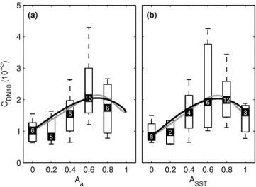
Our observations enable investigation into the relationship between sea-ice drag and ice fraction. Figure 2 showsCDN10
plotted as a function ofAfor allflux-runsand for all methods used to deriveA(see Appendix B). These are ice fraction de-rived via albedo (Aa)and via surface temperature (ASST) us-ingno ice transitiontie points set according to inspection of our in-flight videos and also to values expected theoretically (ASST2)or as previously observed (Aa2). The observational
data are partitioned into ice fraction bins using intervals inA of 0.2 (corresponding to a total of six bins). This interval was chosen as it permits a relatively large number of data points in each bin (between 11 and 65; see Fig. 2), whilst providing a sufficient number of bins to assess the sensitivity ofCDN10
toA. The distribution of values within each bin is represented by the median, the interquartile range, and the 9th and 91st percentiles.
In all four panels in Fig. 2, the lowest median drag coeffi-cients are found at the upper and lower limits of ice fraction (in theA=0, 0.2, and 1 bins), whilst the highest median drag coefficients are in the 0.6 and 0.8 bins. This describes a uni-modal, negatively skewed distribution (i.e. with a longer tail towards lowerA). This distribution qualitatively conforms to the L2012 parametrisation using typical parameter settings (this is revisited in Sect. 4.3). Across all ice fractions our re-sults lie within the range of those obtained in previous studies (see review in Sect. 1 and Andreas et al., 2010).
The small interquartile range inCDN10 evident in Fig. 2 in theA=0 bin reflects the small variability in wind veloc-ity during the field campaign, with run-averaged wind speeds averaging 7 m s−1(close to the climatological mean for the
Arctic summer), peaking at 13 m s−1(see Table 2) and
off-0 0.2 0.4 0.6 0.8 1 0
1 2 3 4 5
Aa C DN10
(10
−3
)
40 49 34 16
11 34
0 0.2 0.4 0.6 0.8 1 ASST
64 45 19
19
17 26
0 0.2 0.4 0.6 0.8 1 0
1 2 3 4 5
Aa2 C DN10
(10
−3
)
43 48 35 17
16 25
0 0.2 0.4 0.6 0.8 1 ASST2
65 51 19 16
20 19
(a) (b)
(c) (d)
Figure 2. CDN10 as a function of ice fractionA:(a) Aa (from albedo);(b)ASST(from sea surface temperature with ano ice tran-sitionat−3.4◦C;(c)Aa2(from albedo with alternative tie points);
and(d)ASST2(from SST with ano ice transitionat−1.8◦C). Ob-servational data are arranged in ice fraction bins of interval 0.2. Box and whisker plots show the median (black square), interquar-tile range (boxes), and 9th and 91st perceninterquar-tiles (whiskers) within each bin. The number of data points within each bin is indicated at the bin-median level. The L2012 scheme is illustrated by curves an-chored at our observed values forA=0 andA=1, using parameter settings E2016A (black curve) and E2016B (grey curve) in Table 1.
ice). Note that over the open ocean (away from ice), surface roughness is a strong function of wave height and therefore wind speed. Our bin-averaged CDN10 values over open sea
water compare well with those expected by inputting ob-served wind speeds into the well-established COARE bulk flux algorithm of Fairall et al. (2003). Values derived from COARE Version 3.0 consistently lie within the interquartile range.
For data points over continuous ice (A=1) our observed
median values of CDN10 are towards the lower end of the
range for large flat floes given in Overland (1985) of 1.2–3.7. However, relative to that forCDN10w, there is a high degree
of variability inCDN10iwithin bins. This reflects significant
heterogeneity in ice conditions and hence roughness, as pre-viously discussed (e.g. Overland, 1985), and as was visually apparent from the aircraft throughout our field campaign. For this reason, over uninterrupted iceCDN10 is region specific, unlike over open water. In our observations these values are indeed found to vary systematically and considerably with location and this is investigated further below. Even greater scatter inCDN10is apparent within the intermediate ice
frac-tion bins (0.2, 0.4, 0.6 and 0.8) as form drag here is affected not only by variability in ice roughness, but also by variabil-ity in the frontal area of floes (governed by floe size and free-board height). Furthermore, the upper limit of ice roughness is likely to be greater here due to deformation as a result of waves and floe advection (Kohout et al., 2014).
It is apparent from Fig. 2 that our results are qualitatively similar for all derivations ofA. In particular, apart for some minor shifts inCDN10due to the rearrangement of data points between adjacent bins, the impact of varying theno ice tran-sitiontie point is small – compare panel (a) with panel (c) and panel (b) with panel (d). This implies that our results are relatively robust.
4.2 Variability within the data set
To further explore the observed sensitivity ofCDN10withA as well as the scatter inCDN10 within ice fraction bins, we
now focus on subsets of the data. Given the dependence of surface roughness not only on ice fraction but also on sea-ice properties, a logical divide would be based on location. As is apparent in Fig. 1, the flights were conducted either to the northwest of Svalbard in Fram Strait or to the southeast of Svalbard in the Barents Sea. Conveniently, this split appor-tions approximately equal numbers of data points to each lo-cation. Results from Fram Strait are shown in Fig. 3, whilst those from the Barents Sea are shown in Fig. 4. Given the lack of sensitivity of results to varying theno ice transition tie point, onlyAaandASSTare shown here.
Significant differences in the distribution ofCDN10 as a
function ofAfor these two locations are apparent, especially towards the higher ice fractions. The Barents Sea is char-acterised by far greater values ofCDN10 for A≥0.6, with medianCDN10≈2.5×10⁻³atA=1, compared to less than 1.2×10⁻³in Fram Strait (note that at lower ice fraction there
is more consistency inCDN10between the locations). These
differences imply rougher sea-ice conditions in the Barents Sea, a result that might be expected given the typically thin-ner ice, a less sharp ocean–ice transition here (i.e. a geo-graphically larger MIZ, see Fig. 1), and greater variability in the position of the ice edge in the Barents Sea during the field campaign – suggestive of ice melt, deformation, and change-able ice conditions. Such heterogeneity is reflected by the considerably greater scatter inCDN10, whilst the wider MIZ
0 0.2 0.4 0.6 0.8 1 0
1 2 3 4 5
Aa C DN10
(10
−3
)
8 16
25 10
10 19
0 0.2 0.4 0.6 0.8 1 ASST
10 29 14
13 11
20
(a) (b)
Figure 3.As in Fig. 2, but for Barents Sea flights only (see Table 2 for details of flights).
0 0.2 0.4 0.6 0.8 1 0
1 2 3 4 5
Aa C DN10
(10
−3
)
32 33 9 6 1
15
0 0.2 0.4 0.6 0.8 1 ASST
54 16 5
6 6 6
(a) (b)
Figure 4.As in Fig. 2, but for Fram Strait flights only (see Table 2 for details of flights).
0.6, and 0.8) for the Barents Sea data (around 69 %) com-pared to Fram Strait data (35–51 %).
The systematic differences in ice conditions between these locations are also apparent in flight videos and photographs. Figure 5 shows images from two Barents Sea flights: a photo-graph from the port-side of the FAAM aircraft during Flight B760 and a still taken from the forward-looking video cam-era 10 days later during MASIN Flight 185 (see Fig. 1 for image locations). Each of these images is representa-tive of sea-ice conditions associated with the highest indi-vidual values ofCDN10observed during each flight (4.7 and 5.7×10⁻³respectively) and correspond to ice fractions of ∼0.8 and∼0.6, respectively. The ice morphology depicted
in the two photos is comparable, constituting relatively small, broken floes (of order tens of metres in scale) with raised edges implying collisions between the floes. Whilst evidently
Figure 5. (a) Photograph taken from the FAAM aircraft during Flight B760flux-runmarked with an arrow in Fig. 7; and(b)still from video recorded from the MASIN aircraft during Flight 185. The image locations are marked in Fig. 1.
widespread in the Barents Sea MIZ, such conditions are not apparent in video footage and photographs made during two of the three Fram Strait flights (182 and 183). During these flights, ice morphology in the MIZ appears quite different: consisting of larger floes often separated by large leads and a more distinct ice edge (as depicted for Flight 182 in Fig. 6). The jagged, small floes illustrated in Fig. 5 are associated with highCDN10 values. Such conditions in the wintertime
Figure 6.Photograph taken from the MASIN aircraft between legs 3 and 4 during Flight 182 at an altitude of∼100 m. The location is marked in Fig. 1.
Figure 7.Spatial maps of ice fraction (a)Aa, (b)ASST, and(c) drag coefficientCDN10for allflux-runsduring FAAM Flight B760. The background greyscale shading is OSTIA sea-ice concentration (lighter shades indicating higher ice concentrations).
Sea flights. Note that whilst the relevant Flight 182 and 183 legs overlap, Flight 184 was conducted further east (Fig. 1).
To delve more deeply into the relationship betweenCDN10 and ice fraction, we now examine two particular flights – one from each research aircraft. We focus on the flights with the greatest number offlux-runsfrom each aircraft: FAAM Flight B760 and MASIN Flight 181 (Table 2). Figures 7 and 8 show distributions ofAa,ASST, andCDN10for allflux-runs in map form for both flights. Note there is generally good agreement between Aa andASST where data are available
for both (a pyranometer malfunction during B760 limits the availability of Aa). In Flight 181, the aircraft traversed the
relatively broken ice immediately southeast of Svalbard, and over the ice edge and open water further south. The B760 leg traversed north–south over the ice edge at a similar lo-cation. From these figures it is apparent that in general the highest values ofCDN10relate to MIZ conditions. This is es-pecially clear for Flight B760, due to the simple gradient in ice fraction; towards the south,CDN10is small over open wa-ter; moving northward over the MIZCDN10increases and ex-hibits more variability, reflecting typically heterogeneous ice conditions in the MIZ, and for the northernmost runsCDN10
decreases again as more consolidated pack ice is encountered (Fig. 7). As discussed above, sea-ice conditions during the B760 flux-runfor which peak CDN10 is observed (arrow in
Fig. 7) are captured in the photograph shown in Fig. 5a.
Figure 8.Spatial maps of ice fraction(a)Aa, (b)ASST, and(c) drag coefficientCDN10for allflux-runsduring MASIN Flight 181, as Fig. 7.
Figure 9 showsCDN10as a function ofAfor Flight 181. The distribution is similar to that described previously, with CDN10peaking in theA=0.6 and 0.8 bins. Comparing Fig. 9 with Fig. 3 shows that drag coefficients are towards the lower end of the range for the Barents Sea. Note that a similar plot is not shown for Flight B760 due to the sparsity of data. Of all our flights only 181 provides sufficient data across the range of ice fractions to make presentation in this form worthwhile. 4.3 Validation and modifications to the L2012
parametrisation
The curves shown in Figs. 2, 3, 4, and 9 represent the L2012 parametrisation. They result from setting the observed me-dianz0w,CDN10w, andCDN10i in Eq. (12) – to fix the end
points of the curves – then adopting new parameter settings for the form component of drag,CDN10f. These were chosen to provide a good fit to our observational results whilst also largely satisfying previously gathered empirical evidence. In fact, the parameter settings recommended by L2012 provide a near-satisfactory fit to our observations, and only minor op-timization is recommended.
Of the parameters dictating the form component of the drag coefficient (CDN10f; see Eq. 11), hmin, hmax, Dmin,
Dmax, andβare all appointed in L2012 according to previous observations. Values assigned to the effective resistance co-efficientce and sheltering parametersare considerably less well verified, making them preferential for tuning. Increas-ingsfrom the value recommended in L2012 such as to bring about a better fit to our data has minimal effect onCDN10
0 0.2 0.4 0.6 0.8 1 0
1 2 3 4 5
Aa C DN10
(10
−3
)
6 15
5
5 6
0 0.2 0.4 0.6 0.8 1 ASST
3 12 6 4
2 8
(a) (b)
Figure 9.As in Fig. 2, but for Flight 181 only (see Table 2 for flight details).
The fit using the E2016A settings is not perfect. In par-ticular, there is a suggestion that for the full data set (Fig. 2) CDN10is underestimated at high ice fraction (theA=0.8 and 0.6 bins) and overestimated at A=0.2. As indicated by our results and those of previous studies,CDN10at high ice
frac-tions is governed by sea-ice morphology and as such its vari-ability is large and location dependent. Consequently, dis-crepancies here are unsurprising. A possible explanation for the overestimate at lower ice fractions is that the parametri-sation does not take into account the attenuating effect of sea ice on waves (e.g. Wadhams et al., 1988). To compute the form drag coefficient (Eq. 11) we use observedz0w, av-eraged over allflux-runswhereA=0. In the MIZ, this as-sumes these values to be representative of the water between ice floes. However, given the sensitivity ofz0to wave ampli-tude (discussed in Sect. 4.1) and the attenuation of waves in the MIZ, these values may in fact be overestimates, leading to an overestimation ofCDN10.
With these discrepancies in mind, we define a second set of parameters, for which β (a morphological exponent de-scribing the dependence ofDi– the floe dimension – onA) is adjusted as well asce. In L2012 aβ value of 1 is derived empirically by fitting their parametrisation for Di (Eq. 17)
to laser scanner observations from Fram Strait obtained by Hartmann et al. (1992) and Kottmeier et al. (1994). However, L2012 also found that by changing onlyβ, their parametrisa-tion was able to explain the variability inCDN10derived from various observational sources. For example, β=1.4 better represented observations made during REFLEX in the east-ern Fram Strait (Hartmann et al., 1994), whilstβ=0.3 bet-ter represented observations made in the Antarctic (Andreas et al., 1984) and the western Fram Strait (Guest and David-son, 1987). Reducing β has the effect of reducing Di and
consequently amplifyingCDN10for all ice fractions, though
particularly towards the higher fractions (though note thatDi
will always eventually converge onDmaxatA=1, accord-ing to Eq. 17). Consequently, settaccord-ing a low value forβ helps explain particularly high drag coefficients atA≈0.8, justi-fying our second parameter set, for which we reduceβ to 0.2 (the lowest value recommended in L2012) in addition to further reducingce to 0.13, to account for the reduction in
CDN10 across all values of Awhich comes from reducing β. Figure 2 shows that these parameter settings (E2016B in Table 1) provide in general a marginally better fit to the com-plete data set than the E2016A settings.
The parametrisation is shown to also provide a generally good fit to subsets of the data. For example, the black and grey curves in Figs. 3 and 4 (the Barents Sea and Fram Strait subsets) denote as before the scheme using the E2016A and E2016B parameter settings respectively, and fit well despite the different ice morphologies and related contrasting val-ues ofCDN10atA=1. For the Barents Sea observations, the curve again passes through the interquartile range of all bins – though a little higher than the median values – both for AaandASST. For the Fram Strait observations there is good agreement in the case ofAa, whilst forASSTthe form drag
is generally overestimated. Finally, the parametrisation also provides an accurate representation of the Flight 181 obser-vations (Fig. 9). It is important to note that the success of the scheme for different localities characterised by different ice conditions depends crucially on an accurate representation ofCDN10 atA=1. As mentioned in Sect. 2.3, in Eq. (12), CDN10atA=1 is provided byCDN10i, defined in L2012 as
the skin drag over sea ice. However, given that over rough, ridged sea ice, there is a form drag component in addition to skin drag, this term is more suitably expanded and expressed asthe total (skin and form) drag over continuous sea ice, and considered to be a variable quantity, dependent on ice condi-tions.
As discussed in Sect. 4.2, our observations suggest that ice conditions in the MIZ characterised by relatively small, unconsolidated “pancake” ice floes at intermediate ice con-centrations are characterised by higher drag coefficients than larger floes. The roughness extends locally to the highest ice concentrations, suggesting a case could be made for the use ofDiat intermediate ice fractions as a proxy for local MIZ
surface roughness. Although this is partially implicit in the L2012 scheme in the sense that it accounts for smaller floes exerting greater form drag for a given ice concentration due to a greater frontal area (see Eq. 11), it seems likely given our observations that smaller floes are often associated with largerCDN10due to other, unaccounted-for reasons – for ex-ample, greater deformation and ridge-forming as a result of more frequent floe collisions due to smaller gaps between the floes or to floe advection caused by reduced ocean wave at-tenuation in areas of smaller floes. Note that this additional roughness corresponds to that discussed in the above para-graph as requiring inclusion in theCDN10iterm in Eq. (12).
the literature (Garbrecht et al., 2002; Andreas, 2011), though there is as yet no clear solution to this problem, and further progress in this area is beyond the scope of this study; see Conclusions for recommendations for future work.
5 Implications and parametrisation recommendations It is clear that the physically based parametrisation of L2012 qualitatively fits our observations of surface drag (i.e. mo-mentum exchange) over the MIZ very well. The recom-mended settings provided by L2012 (see Table 1) also quan-titatively fit our observations well, although with some tuning ofce(the effective resistance coefficient) and, optionally,β(a sea-ice morphology exponent) this fit can be improved when compared to median CDN10 values – see Figs. 2–4 and 9.
We recommend two settings for the L2012 parametrisation: E2016A withce=0.17 andβ=1 and E2016B withce=0.1
andβ=0.2 (see Table 1). The E2016B setting enhances the negative skew of theCDN10distribution, increasing
(decreas-ing) values at high (low) ice concentrations. These settings are illustrated as the black and grey lines in Figs. 2–4 and 9.
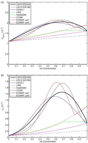
Our recommended L2012 settings are also plotted in Fig. 10 to allow a comparison against several other parametrisations used in numerical sea ice, climate or weather prediction models. Figure 10a shows the effective 10 m neutral drag coefficient for a grid square with the ice concentration indicated, i.e. it is an effectiveCDN10
calcu-lated proportionally for that mix of water and sea ice. To al-low a direct comparison, the drag coefficient over open wa-ter,CDN10w, is set to 1.1×10⁻³for all the algorithms. This
value is appropriate for low-level winds of about 5 m s−1. It is
simply chosen for illustrative purposes; similar illustrations result for other values ofCDN10w. Figure 10b shows the
ef-fective roughness length – derived from the efef-fectiveCDN10
using Eq. (3) – as a function of sea-ice concentration. In ad-dition to our recommended L2012 parametrisation settings, we also show those set as default in the sea-ice model CICE version 5.1 (see Tsamados et al., 2014; Hunke et al., 2015). In these, ce=0.2, β=1, and the ice flow sheltering con-stants=0.18 (see Table 1). Note that there is a typograph-ical error in Table 2 of Tsamados et al. (2014), where the parameters csf andcsp are listed as equal to 0.2 (implying
ce=1) when these should have been listed as equal to 1 (M.
Tsamados, personal communication, 2015). When the cor-rected values are used, the CICE5.1 parametrisation matches our observations reasonably well (Fig. 10); although it does not account for the negative skew in the observations.
The ECMWF introduced a new parametrisation of surface drag over sea ice in cycle 41 of the Inte-grated Forecast System, which became operational on 12 May 2015. This introduces a variable sea-ice roughness lengthz0i =max[1, 0.93(1−A)+6.05e−17(A−0.5)
2
]×10−3
(see ECMWF documentation and Bidlot et al., 2014). This parametrised an increase in drag coefficient over the MIZ
0 0.1 0.2 0.3 0.4 0.5 0.6 0.7 0.8 0.9 1 0
0.5 1 1.5 2 2.5 3
Ice Concentration
CDN10
(10
−3
)
(a)
L2012 E2016A L2012 E2016B CICE5.1 LIM3 HadGEM3 CCSM ECMWF cy41 ECMWF cy40
0 0.1 0.2 0.3 0.4 0.5 0.6 0.7 0.8 0.9 1 0
0.2 0.4 0.6 0.8 1 1.2 1.4 1.6 1.8 2
Ice Concentration
z0
(10
−3
)
(b)
L2012 E2016A L2012 E2016B CICE5.1 LIM3 HadGEM3 CCSM ECMWF cy41 ECMWF cy40
Figure 10. (a)Effective sea-ice drag coefficient and (b) derived effective roughness length as a function of ice concentration. Parametrisations shown are: Lüpkes et al. (2012) with settings as recommended here, namely L2012 E2016A with ce=0.17 and
β=1 (black), and L2012 E2016B with ce=0.1 and β =0.2 (grey); the default L2012 settings used in CICE5.1 (blue) as de-scribed in Tsamados et al. (2014); the LIM3 interpolation (blue dash-dotted); the HadGEM3 default used in the Met Office Unified Model (green); the CCSM (and CAM5) interpolation (magenta); the ECMWF cycle 41 function (red) and the previous ECMWF cycle 40 interpolation (red dashed). See Table 1 for other L2012 settings.
which was inspired by the observations described in Andreas et al. (2010), so is consistent with L2012, and is close to our recommended settings for L2012 (Fig. 10).
All of the other parametrisations that are illustrated lin-early interpolate between the drag coefficient over open wa-ter and constant values for CDN10i (or z0i). Consequently,
they appear as straight lines in Fig. 10a. In the case of the ECMWF (cycle 40 and earlier) a constantz0i=1×10⁻³m
default setting in the ECHAM climate model (see Lüpkes et al., 2013) and in the WRF numerical weather predic-tion model (Hines et al., 2015) – not shown in Fig. 10. In the CCSM (Community Climate System Model) and CAM5 (Community Atmospheric Model) CDN10i is set to 1.6×10⁻³ (see Neale et al., 2010) and in LIM3 (the
Louvain-la-Neuve Sea Ice Model)CDN10iis set to 1.5×10⁻³
by default (see Vancoppenolle et al., 2012). Previous versions of the CICE sea-ice model also used a constant z0i set as
0.5×10⁻³m. The Met Office use separate constant values
for “the MIZ” (set at A=0.7) and “full sea ice” and then linearly interpolate. For their HadGEM3 climate model both z0iandz0MIZare set to 0.5×10⁻³m for version 4.0 of their
Global Sea Ice (GSI) configuration, as illustrated in Fig. 10; while for UKESM1, using GSI6.0, much higher values of z0i=3×10⁻³m andz0MIZ=100×10−3m are planned (see
Rae et al., 2015). These are equivalent toCDN10values of 2.4 and 7.5×10⁻³, respectively, so arenotsupported by our
ob-servations (see Fig. 2).
Examining Fig. 10, only the new (cycle 41) ECMWF parametrisation is qualitatively and quantitatively compara-ble to our recommended settings of the L2012 parametrisa-tion. At present most numerical weather and climate predic-tion models do not have a maximum in drag coefficient over the MIZ. Consequently, they are not consistent with our ob-servations, nor those of relevant previous compilations (e.g. Andreas et al., 2010; L2012).
It is clear that in configuring sea-ice models,CDN10over
sea ice has commonly been used as a “tuning parameter”. In fact it was specifically treated as such in the model sen-sitivity studies of, for example, Miller et al. (2006) and Rae et al. (2014). Miller et al. (2006) used the CICE model in standalone mode and varied three parameters widely, in-cluding CDN10 between 0.3–1.6×10⁻³, in an optimisation exercise. They found significant variability in extent and thickness across their simulations and concluded that de-termining an optimal set of parameters depended heavily on the forcing and validation data used. Rae et al. (2014) carried out a comprehensive fully coupled atmosphere– ocean–ice modelling sensitivity study, testing a large num-ber of sea-ice-related parameter settings within their obser-vational bounds. They found statistically significant sensitiv-ity to the two sets of roughness length settings they tested: “CTRL” (z0i=0.5×10⁻³ and z0MIZ=0.5×10⁻³m) and
“ROUGH” (z0i=3×10⁻³andz0MIZ=100×10−3m). The
rougher settings (also consistent with those in the Met Of-fice global operational model) generally lead to simulations with a better sea-ice extent and volume compared to obser-vations. However, we would note again that they are not con-sistent with our observations. Instead, our results would sug-gest these seemingly required large roughness lengths must be compensating for other deficiencies in the model configu-ration.
As discussed in Sect. 2, the exchange of momentum be-tween the atmosphere and sea ice depends heavily on sea-ice
morphology, thickness, and concentration. Prior to this study, observations of sea-ice drag were relatively limited, espe-cially for the MIZ (i.e. for ice fractions 0< A <1). Conse-quently,CDN10has not previously been well constrained by observations. Our data set doubles the number of observa-tions available over the MIZ and is based on independent re-search platforms and analysis procedures to previously pub-lished data sets. Importantly, our results are broadly con-sistent with these previous observational compilations (e.g. Andreas et al., 2010; and L2012). This corroboration pro-vides further confidence in our recommendations. In short, CDN10is now better constrained and we recommend that its
parametrisation is consistent with our results.
6 Conclusions
We have investigated surface momentum exchange over the Arctic marginal ice zone using what is currently the largest set of aircraft observed data of its kind. Our results show that the momentum exchange is sensitive to sea ice concentra-tion and morphology. Neutral 10 m surface drag coefficients (CDN10)are derived using the eddy covariance method and Monin–Obukhov theory, and two methods (which provide qualitatively similar results) are adopted for the derivation of ice fraction from our aircraft observations. After averag-ingCDN10 data into ice fraction bins, the roughest surface
conditions (characterised by the highest surface drag coeffi-cients) are typically found in the ice fraction bins of 0.6 and 0.8, while the smoothest surface conditions tend to be over open water and sometimes (dependent on sea-ice conditions) over continuous sea ice. Consequently, a good approxima-tion for our observedCDN10as a function of ice concentra-tion is provided by a negatively skewed distribuconcentra-tion, in gen-eral agreement with previous observational studies (Hartman et al., 1994; Mai et al., 1996; Lüpkes and Birnbaum, 2005). However, we have found systematic differences in roughness between different locations. Over deformed, 10 m scale pan-cake ice in the Barents Sea, drag coefficients are considerably greater than over relatively homogeneous, non-deformed sea ice in Fram Strait. This dependence on ice morphology gov-erns the magnitude and variability with ice fraction ofCDN10,
and is likely to be the major cause of the considerable scatter inCDN10within each ice fraction bin.
CDN10=(1−A) CDN10w+ACDN10i
+Ahf DiS
2
c
ce 2
" ln2(h
f/z0w)
ln2(10/z0w) #
. (20)
The final term on the right-hand side of this equation ex-presses the form drag component, and is derived following the theory of pressure drag exerted on a bluff body. This ex-pression can be simplified following L2012 to be given as a function of only ice fractionAand tuneable constants via Eqs. (15) to (18). In this simple form, the scheme provides a generally accurate representation of the observed distribution ofCDN10as a function of sea-ice fraction. The agreement is
optimized by adopting minor parameter adjustments to those originally recommended in L2012. These new settings are la-belled as E2016A and E2016B in Table 1. E2016B arguably provides a better fit, though with values ofceandβwhich are at the limit of those physically plausible according to obser-vations, whereas for E2016A these values are well within the confines of those observed. The scheme is shown to be ro-bust, its success holding for subsets of our data (e.g. for each of the Barents Sea and Fram Strait locations, and for the sin-gle flight with the greatest number of data points) so long as it is anchored atA=1 by an observed value forCDN10i.
Given the success of a sophisticated scheme such as that of L2012, the representation of sea-ice drag in many weather and climate models seems crude by comparison, withCDN10
often set with little consideration of physical constraints and instead used as a tuning parameter. Our comprehensive ob-servations provide the best means yet to constrain parametri-sations of CDN10 over the MIZ. They clearly imply that linearly interpolating between the open water surface drag (CDN10w)and a fixed sea-ice surface drag (CDN10i), as many
parametrisations do, is not physically justified or represen-tative. It is recommended that, as a minimum, parametrisa-tions incorporate a peak inCDN10 within the rangeA=0.6 to 0.8 (as a guide, in the 0.6 and 0.8 ice fraction bins of our observations,CDN10has a mean interquartile range of 1.25
to 2.85×10⁻³for all data – i.e. averaged across both bins
for all panels in Fig. 2). Note that the precise peak value will vary with sea-ice morphology and, as found in Lüpkes
and Gryanik (2015), stratification. Though sophisticated, the simplest form of the L2012 scheme is not computationally complex (having only one independent variable,A) and is recommended for adoption in weather and climate models.
The sensitivity ofCDN10 to ice fraction is now well es-tablished. Consequently, we recommend that future work fo-cuses on the remaining major source of uncertainty: sensi-tivity to ice morphology. Our results suggest that the simpli-fication of the L2012 scheme by parametrising floe dimen-sion (Di)and freeboard (hf)in its expression for form drag on floe edges usingAprovides sufficiently accurate results. Even so, as discussed above, floe size and ice morphology has a major impact on surface roughness and a more so-phisticated representation of this should benefit sea-ice and climate simulations. In particular, this study demonstrates that setting an appropriate value ofCDN10atA=1 is vital to the success of the L2012 parametrisation; given the ob-served variation with location (and hence ice conditions), a constant value forCDN10 atA=1 is clearly unsuitable for simulations over large areas such as the entire Arctic. Here, we simply varyCDN10iin the L2012 scheme to reflect the
ob-served location-dependent ice roughness atA=1. In sea-ice or climate models, perhapsCDN10atA=1 should be deter-mined from sea-ice model output – for example, Tsamados et al. (2014) account for form drag on ice ridges. In oper-ational models, perhapsCDN10 atA=1 should be derived from sea-ice thickness observations (e.g. from CryoSat-2).
Our observations indicate that floe size is a governing fac-tor in local variations of sea-ice roughness, even at the high-est ice fractions. Consequently, to account for MIZ rough-ness associated with local ice conditions an option could be to accentuate the dependency ofCDN10 on floe size by ex-pandingCDN10i to incorporate both the skin drag term and an additional “local” sea-ice form drag term which would be inversely proportional to a representative value ofDi(e.g. av-erageDiat a given ice fraction). To pursue such an approach
Appendix A: Quality control of momentum flux data In order to remove unsuitable data, a quality control proce-dure is utilised. This proceproce-dure follows previous studies (e.g. French et al., 2007; Petersen and Renfrew, 2009; Cook and Renfrew, 2015) and involves the visual inspection of a series of statistical diagnostics describing the variability of the per-turbation wind components along eachflux-run. “Bad” data points arise as a result of instrument malfunction or the viola-tion of assumpviola-tions made in the methodology – notably that the turbulence is homogeneous along each run. The criteria that determine a “good” run are as follows:
The power spectra of the along-wind velocity component should have a well-defined decay slope (close tok−5/3for wavenumberk).
The total covariance of the along-wind velocity and verti-cal velocity should be far greater in magnitude than that of the cross-wind velocity and vertical velocity (which should be small), indicating alignment of the shear and stress vec-tors.
The cumulative summation of the covariance of the along-wind velocity and the vertical velocity should be close to a constant slope, indicating homogeneous covariance.
The cospectra of the covariance of the along-wind ve-locity and the vertical veve-locity should have little power at wavenumbers smaller than about 10−4m−1, implying that
mesoscale circulation features are not contributing signifi-cantly to the stress.
The cumulative summation of the cospectra should be shaped as ogives (“S”-shaped, with flat ends) implying that all of the wavenumbers that contribute to the total stress have been sampled and again that mesoscale features are not present.
Examples of “good” and discarded runs are illustrated in Fig. A1 (where theflux-runlength is∼9 km). In the “good” example, there is little cross-wind spectral power and the cu-mulative summation has a near-constant slope indicating ho-mogeneous turbulence structure along the length of the run. The “S”-shaped ogives and lack of power at small wavenum-bers in the cospectra suggest that the turbulence is fully cap-tured and that the signal is “unpolluted” by mesoscale cir-culations. For this typical case, the majority of energy is in eddies ranging from about 30 to 500 m in size, with no en-ergy at all for wavelengths over 2500 m. This information helps inform a suitable run duration, since it is important that the runs are long enough to capture several eddies of sizes at least across the dominant range of the spectrum. On the other hand, lengthening runs reduces the number of data points and increases the risk of sampling organised mesoscale features instead of pure turbulence.
Note that five differentflux-rundurations were trialled us-ing a sample of the data set. These durations varied between the two aircraft (according to their mean flight speed) in or-der that they correspond to lengths of approximately 3, 6, 9, 12, and 15 km. Using the above quality control procedure it
10−4 10−3 10−2 10−1 100 −0.5
0 0.5 1 1.5
Ogives
uw
Wavenumber (m−1)
10−4 10−3 10−2 10−1 100 −0.3
−0.2 −0.1 0 0.1
Cospectra
uw
(m
2 s
−2
)
Wavenumber (m−1)
0 0.2 0.4 0.6 0.8 1 −0.5
0 0.5 1 1.5
Fractional distance
Cum. Summation
uw
10−4 10−3 10−2 10−1 100
Wavenumber (m−1)
10−4 10−3 10−2 10−1 100
Wavenumber (m−1)
0 0.2 0.4 0.6 0.8 1
Fractional distance
Total uw covariance: −991 m2 s−2 Total vw covariance: 12 m2 s−2
Total uw covariance: −223 m2 s−2 Total vw covariance: 344 m2 s−2
Figure A1.Quality control diagnostics for momentum flux (u′w′).
Left column shows a “good” run (Flight 181, leg 2, run 7); right column shows a “bad” run (Flight 181, leg 5, run 11). The rows show (top) the cumulative summation ofu′w′versus distance along
the run, (middle) the frequency weighted cospectra, and (bottom) the ogives (integrated cospectra) both as a function of wavenumber. The cumulative summation is normalised by the total covariance and the ogives by the total cospectra.
was ascertained that a run length of 9 km procures the high-est quality data and so is used here. This is comparable to Weiss et al. (2010) and Fiedler et al. (2010) who used 8 and 8.8 km; and a little shorter than Petersen and Renfrew (2009) and Cook and Renfrew (2015) who used 12 km.
Appendix B: Deriving ice fractionAfrom the aircraft observations
Two different remote sensing techniques are used to derive estimates ofice fractionAfrom the aircraft observations, us-ing proxies based on albedo and surface temperature. These techniques rely on sea ice being more reflective and colder than sea water. In both approaches the proxy is linked toA using two tie points: one at theno ice transitionbetween open water and the onset of ice (A→0) and another at theall ice transitionbetween continuous ice and the appearance of some water (A→1). This allows an estimate of ice
concen-tration for each data point, accounting for the fact that each measurement may sample multiple floes. Ice fraction is then provided for each measurement by
AX=
0 for X≤XA→0
(X−XA→0)
(XA→1−XA→0) for XA→0< X < XA→1
1 forX≥XA→1,
whereXis the instantaneous value of the proxy andXA→0
and XA→1 are the tie points for theno ice transition and
theall ice transitionrespectively. Note that the recorded air-craft data (1 Hz for the relevant diagnostics) and approxi-mate mean aircraft speed for straight and level runs (60 and 100 m s−1for MASIN and FAAM respectively) translates to
each measurement point sampling over a distance of 60 and 100 m (≫Dmin), respectively. We average over the 9 km run
to obtain a representative ice fractionA.
Albedo is calculated from measurements of the upward and downward components of the shortwave radiative flux: a=SWU/SWD.Aais derived using tie pointsaA→0=0.15
andaA→1=0.85, which were chosen following careful
re-view of video footage from four flights (two from each air-craft: MASIN 182 and 185; FAAM B761 and B765). It is accepted that these tie points are approximate and may vary depending on ice conditions; however, there is good agree-ment between the flights for which video footage was avail-able. While these values are broadly consistent with text-book albedo values (e.g. Curry and Webster, 1999), aA→0
is towards the upper end of the expected range, so an alter-native albedo-derived ice fraction, Aa2, is calculated using
aA→0=0.07 (matching that used to approximate freezing
point in the Weddell Sea in Weiss et al., 2012). A limitation of the albedo approach is thatAawill be underestimated for
semi-transparent thin ice, as measurements will be affected by the lower albedo of the sea water below.
In the SST approach, a lower tie point of SSTA→0= −3.4◦C was ascertained following inspection of the flight
videos. It is recognised that this value is lower than might be expected given typical ocean salinity. Indeed, salinity mea-surements made by the RRS James Clark Ross as part of the ACCACIA field campaign suggests typical values of be-tween 30 and 35 (a little fresher than is typical, likely as a result of spring melt), implying a freezing point of about
−1.8◦C. It is possible this discrepancy may be due to a
cool skin being measured by the aircraft’s radiometers. In the vicinity of the MIZ, cool skin temperatures are likely to be a result of the top few centimetres of the ocean containing small fragments of ice (e.g. frazil) as was observed during the flights. In addition, the radiatively driven “cool skin effect” (Fairall et al., 1996) may also contribute. To account for this uncertainty, we also calculate two different ice fractions us-ing the SST approach;ASSTuses the lower value suggested
by the video footage (−3.4◦C), whileASST2 uses the
theo-retical value based on observed salinities (−1.8◦C).
Due to the thin-ice problem, the SST approach is arguably more suitable than the albedo approach at prescribing the on-set of ice with a suitable fixedno ice transition(so long as a suitable value is determined). However, there is a funda-mental problem in assigning an SSTall ice transitionthat is suitable across multiple flights. This is because the surface temperature over continuous ice varies greatly according to the atmospheric conditions. Using a fixed value for SSTA→1
could therefore lead to inconsistencies between flights under
0 0.2 0.4 0.6 0.8 1
0 0.2 0.4 0.6 0.8 1
0 0.2 0.4 0.6 0.8 1
A
a ASST
0 0.2 0.4 0.6 0.8 1
A
a
Aa | ASST
Aa | ASST2
Aa2 | ASST
Aa2 | ASST2
(a) (b)
Figure B1.Ice fraction calculated from aircraft observations using the surface temperature method (ASST)plotted against that using the albedo method (Aa).(a)Data points for every run (dots) and linear regression (black line) are shown, using the default criteria for both methods (aA→0=0.15 and SSTA→0= −3.4◦C). Dots are coloured according to the OSTIA satellite-derived ice fraction, and the one-to-one line (grey) is shown.(b)Linear regressions of all combinations of observation-derivedAaandASST.
different weather conditions; for example overestimatingA in the case of particularly cold ice floes asA→1. Conse-quently, in the SST approach an adjustment of the SSTA→1
tie point using albedo is used, which provides a robust esti-mate of SSTA→1 for any atmospheric conditions. For each
flight, SSTA→1is set equal to the median SST value for all
flux-rundata points whereais within the rangeaA→1±0.05,
i.e. between 0.8 and 0.9. Using this criterion, SSTA→1ranges
from−23.6 to−9.6◦C between flights, with this variability
being a strong function of latitude (the colder values being for the northernmost flights). The suitability of this method is demonstrated by the high level of internal consistency in SST values within theaA→1±0.05 range for each flight, with a
mean standard deviation (averaged across all flights) of only 1.3◦C.
Figure B1 compares the ice fractions estimated using the albedo and SST methods. It shows that there is a near one-to-one relationship betweenAaandASST, with a correlation
coefficient of 0.94, a root-mean-square error of 0.12 and a bias error of 0.03 for the video-assigned values ofaA→0and
SSTA→0. Linear regressions with the alternative tie point
Table B1.Notation.
A ice fraction
α Charnock constant
b smooth-flow constant for the Charnock relation β constant exponent describing the dependence of
DionA
CD drag coefficient
CDN10 drag coefficient for neutral stability at a height
of 10 m
CDNf10 neutral form drag coefficient at a height of 10 m CDNi10 neutral drag coefficient over sea ice at a height
of 10 m
CDNw10 neutral drag coefficient over sea water at a
height of 10 m
ce effective resistance coefficient
cs ice floe shape parameter
cw fraction of the available force acting on each floe
Di cross-wind floe dimension
Dmin,Dmax minimum and maximum cross-wind floe di-mension
Dw distance between floes
fd total force acting on the frontal areas of ice floes within the area
hf freeboard height of floes
hmin, hmax minimum and maximum freeboard height of floes
κ von Karman constant (0.4) N number of floes in areaSt
ρ air density
s ice floe sheltering function constant Sc ice floe sheltering function
St domain area ofNfloes
τ momentum flux
τd momentum flux related to form drag U horizontal wind speed
U10N adjusted 10-m neutral horizontal wind speed
u∗ friction velocity
υ dynamic viscosity
ϕ Monin-Obukhov stability correction z0 roughness length