Hardware Implementation of Vector Control of Induction Motor Drive without Speed Encoder Using an Adaptive Luenberger Based MRAS Observer

(1)

Leonardo Electronic Journal of Practices and Technologies ISSN 1583-1078

Issue 20, January-June 2012 p. 99-114

Hardware Implementation of Vector Control of Induction Motor

Drive without Speed Encoder Using an Adaptive Luenberger Based MRAS

Observer

Karim NEGADI1*, Abdellah MANSOURI2, and Rabeh KOUREK2

1

Laboratory of Energy and Intelligent Systems, Khemis Miliana University, Algeria

2

Laboratory of Automatics and Systems Analysis (L.A.A.S.), Department of Electrical Engineering, E.N.S.E.T. Oran BP 1523 El’ M’naouer, Oran, Algeria

E-mail(s): karim.negadi@yahoo.fr, ammansouri@yahoo.fr *

Corresponding author: Phone: 00213670251890; Fax: 0021346450435

Abstract

Vector control of induction motor drives without mechanical speed sensors

has the attraction of low cost and high reliability. An adaptive Luenberger

style stator flux observers is presented. Therefore, this paper presents a theory

of adaptive Luenberger observers and his capability to compensate for stator

voltage errors and usefully in electrical drivers systems without sensorless.

Keywords

Sensorless control; Induction motor drives; Adaptive Luenberger observers;

MRAS; Modelling; Vector control.

Introduction

Induction motor drives have been thoroughly studied in the past few decades and

many vector control strategies have been proposed, ranging from low cost to high

performance applications. In order to increase the reliability and reduce the cost of the drive, a

great effort has been made to eliminate the shaft speed sensor in most high performance

(2)

induction motor drives where the mechanical speed of the rotor is generally different from the

speed of the revolving magnetic field. The advantages of speed sensorless induction motor

drives are reduced hardware complexity and lower cost, reduced size of the drive motor,

better immunity, elimination of the sensor cable, increased reliability and less maintenance

requirements. The induction motor is however relatively difficult to control compared to other

types of electrical motors. For high performance control, field oriented control is the most

widely used control strategy. This strategy requires information of the flux in motor; however

the voltage and current model observers are normally used to obtain this information.

Generally, using the induction motor state equations, the flux and speed can be

calculated from the stator voltage and current values. The flux is estimated or observed from

the stator voltage equation and the speed is obtained using the estimate flux and the rotor

equation.

The main objective of the research presented in this paper was to analyse and evaluate

of optimum used flux observer (Adaptive Luenberger) in electrical drivers systems without

sensorless. The analysis was done by use of modern control theory and by extensive testing.

The testing was done with Matlab/Simulink software implemented in real time hardware

model.

Material and Method

Dynamic Model of Induction Motor

The fifth order nonlinear state space model of induction motor is represented in the

synchronous reference frame (d-q) by as follows: [2]

(

s s

)

sd s e sq m rdq m e rq

sd R pL i L i pL i L i

v = + − ω + − ω (1)

(

s s

)

sq s e sd m rq m e rd

sq R pL i L i pL i L i

v = + + ω + + ω (2)

(

Rr pLr

)

ird Lr slirq pLmisd Lm slisq

0= + − ω + − ω (3)

(

Rr pLr

)

irq Lr slird pLmisq Lm slisd

0= + + ω + + ω (4)

l r r

em Jp B T

T = ω + ω + (5)

(3)

(

sq rd sd rq

)

m p

em p L i i i i

2 3

T = − (6)

Components of rotor flux are:

sd m rd r

rd =L i +L i

Ψ (7)

sq m rq r

rq =L i +L i

Ψ (8)

From (7) and (8), d- and q- axes rotor currents are:

(

rd m sd

)

r

rd L i

L 1

i = Ψ − (9)

(

rq m sq

)

r

rq L i

L 1

i = Ψ − (10)

Substituting (7)-(10) into (3) and (4) yields:

0 i R L L L R dt d rq sl sd r r m rd r r

rd + Ψ − −ω Ψ =

Ψ (11) 0 i R L L L R dt d rd sl sq r r m rq r r

rq ₋ _Ψ ₋ ₋_ω _Ψ ₌

Ψ (12)

Control Design

If the vector control is established such that q-axis rotor flux is set zero, and d-axis

rotor flux is maintained constant then equations (11), (12), (9), (10), and (6) becomes:

sd m rd =L i

Ψ (13) sd sq r sl i i T 1 = ω (14) 0

i_rd = (15)

sq r m rq i L L

i =− (16)

rq rd r m p em i L L p 2 3

T = Ψ (17)

(4)

sq s e rq r m e rd m rd m s sq s

sd Li

L L dt di L dt d L L i R

v = + Ψ − σ −ω Ψ −ωσ (18)

dt di L i L i L dt di L L dt di L i R

v e mrd e ssd m rq

rq r 2 m sq s sq s

sq= + σ + +ω +ω +

(19)

Proposed Control Scheme

The stator command currents are obtained using equation (13) and the PI control loop

for speed error as follows [4, 5]:

m * rd * sd L

i = Ψ (20)

(

ˆ

)

K

(

ˆ

)

dt

K

i*_sq = _p ω*_r−ω_r + _i

∫

ω_r*−ω_r (21)

where: Kp, Ki are respectively the proportional and integral arbitrary positive gains.

The speed and the current loops are considered to be fast enough to assume that the

actual stator currents are equal to their command inputs (isd=i*sd and isq=i*sq). The command

voltages are generated as follows:

(

i i

)

K

(

i i

)

dt

K

v * _sd

sd 1 i sd * sd 1 p *

sd = − +

∫

− (22)

(

i i

)

K

(

i i

)

dt

K

v_sq* = _p₂ *_sq− _sq + _i₂

∫

_sq* − _sq (23)

For the field oriented control, the following PI gains of the speed adaptive scheme are

selected: Kp=3, Ki=1800.

Model Reference Adaptive Systems (MRAS)

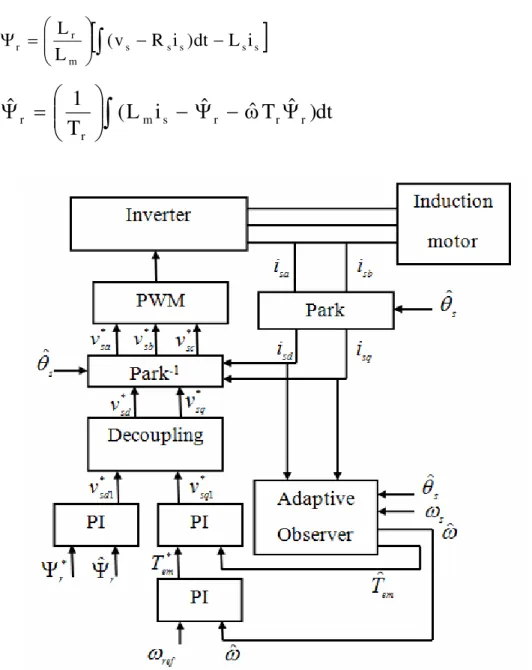
The basic concept of MRAS is the presence of a reference model which determines

the desired states and an adaptive (adjustable) model which generates the estimated values of

the states (figure 1).

The error between these states is fed to an adaptation mechanism to generate an

estimated value of the rotor speed which is used to adjust the adaptive model. This process

continues till the error between two outputs tends to zero [6, 7]. Basic equations of rotor flux

(5)

[

_∫

− −

]

⎟⎟

⎠ ⎞ ⎜⎜ ⎝ ⎛ =

Ψ _s _s _s _s _s

m r

r (v R i )dt L i

L

L (24)

dt

)

ˆ

T

ˆ

i

L

(

T

1 ˆ

r r r

s m r

r

⎟⎟

∫

−

Ψ

−

ω

Ψ

⎠

⎞

⎜⎜

⎝

⎛

=

Ψ

(25)

Figure 1. Integration of adaptive observer and vector control

The reference model (24) is based on stator equations and is therefore independent of

the motor speed, while the adaptive model (25) is speed-dependant since it is derived from the

rotor equation in the stationary reference frame. To obtain a stable nonlinear feedback system,

a speed tuning signal (ε_ω) and a PI controller are used in the adaptation mechanism to generate

the estimated speed. The speed tuning signal and the estimated speed expressions can be

written as [8]:

rq rd rd

rqΨˆ −Ψ Ψˆ Ψ

=

(6)

ω ε ⎭ ⎬ ⎫ ⎩ ⎨ ⎧ ₊ = ω s K K ˆ i p (27)

where: Kp, Ki are the proportional and integral constants, respectively.

Adaptive Luenberger Observer

Luenberger Observer is a deterministic observer with applied to state estimation of

linear time invariant system, the model of induction motor can described by:

) t ( x . C ) t ( y ) t ( u . B ) t ( x . A ) t ( x = + = & (28)

The Luenberger observer is then described by:

) t ( xˆ . C ) t ( yˆ )) t ( yˆ . C ) t ( y ( L ) t ( u . B ) t ( x . A ) t ( xˆ = − + + = & (29)

where L is the observer gain matrix to avoid the use of an expensive speed sensor we estimate

the speed using an adaptive observer based on the MRAS [9].

where: ⎥ ⎥ ⎥ ⎥ ⎦ ⎤ ⎢ ⎢ ⎢ ⎢ ⎣ ⎡ ⎟⎟ ⎠ ⎞ ⎜⎜ ⎝ ⎛ ω − − ⎟⎟ ⎠ ⎞ ⎜⎜ ⎝ ⎛ ⎟⎟ ⎠ ⎞ ⎜⎜ ⎝ ⎛ ω − δ γ − = J T 1 I T L J T I I A r r r m r r _, ⎥ ⎥ ⎥ ⎦ ⎤ ⎢ ⎢ ⎢ ⎣ ⎡ ⎟⎟ ⎠ ⎞ ⎜⎜ ⎝ ⎛ σ = 0 I L 1 B

s , C=

[

I 0

]

, ⎥_⎦ ⎤ ⎢ ⎣ ⎡ = 1 0 0 1

I and _⎥

⎦ ⎤ ⎢ ⎣ ⎡ − = 0 1 1 0 J .

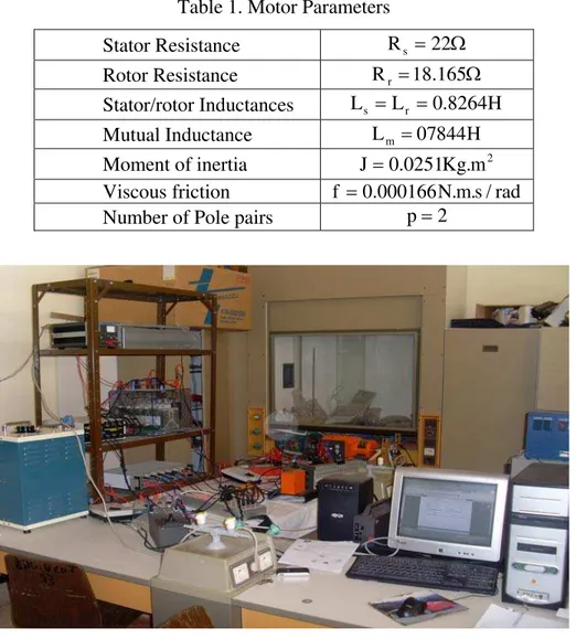
Description of Laboratory Setup

The experimental system consists of two motors, one of which is the driving motor,

and the other serves as the load. The inverters of both motors are controlled by the PC,

providing a possibility for full control for experimental purposes of both the driving motor

and the load motor. The interfacing is made via a dSPACE1104 control board. The

Matlab/Simulink control model can be converted and downloaded to the DSP1104, and then it

can work independently of the Matlab/Simulink environment. During the real-time operation

of the control algorithm, the supervision and capturing of the important data can be done by

the Control Desk software provided with the DSP board. The nominal motor parameters are

(7)

Table 1. Motor Parameters

Stator Resistance R_s =22Ω

Rotor Resistance Rr =18.165Ω

Stator/rotor Inductances L_s =L_r =0.8264H

Mutual Inductance Lm =07844H

Moment of inertia J=0.0251Kg.m2 Viscous friction f =0.000166N.m.s/rad

Number of Pole pairs p=2

Figure 2. Real-time experimental setup

Results and Discussion

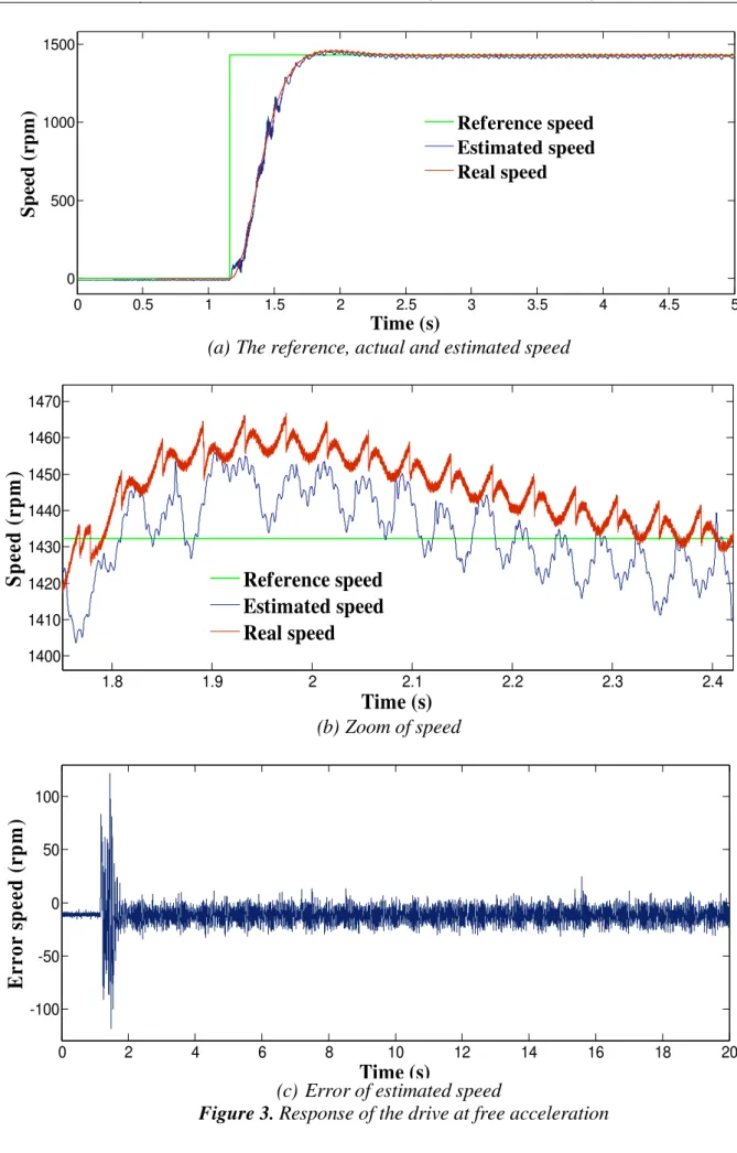
Scenario 1: Free acceleration characteristics

The motor was allowed to accelerate from zero speed to rated speed at no-load. The

steady-state was reached at 1.8 seconds. The waveform of estimated speed show faster

response as compared to its actual counterpart. It can be seen that there is a very good

(8)

0 0.5 1 1.5 2 2.5 3 3.5 4 4.5 5 0

500 1000 1500

Time (s)

Spe

ed (r

pm

)

Reference speed Estimated speed Real speed

(a)The reference, actual and estimated speed

1.8 1.9 2 2.1 2.2 2.3 2.4

1400 1410 1420 1430 1440 1450 1460 1470

Time (s)

Spe

ed (

rpm

)

Reference speed Estimated speed Real speed

(b)Zoom of speed

0 2 4 6 8 10 12 14 16 18 20

-100 -50 0 50 100

Time (s)

E

rro

r s

p

eed

(

rp

m

)

(c) Error of estimated speed

(9)

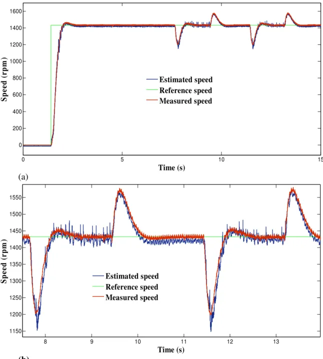
Scenario 2: Free acceleration characteristics

Figure 4 shows the speed-sensorless control performance where the load was applied

and omitted. The estimated speed coincides exactly with the real speed even the load torque

application instant. From these results, it is shown that the proposed speed-sensorless control

algorithm has good performances.

0 5 10 15

0 200 400 600 800 1000 1200 1400 1600

Time (s)

Spe

e

d (

r

pm

)

Estimated speed Reference speed Measured speed

(a)

8 9 10 11 12 13

1150 1200 1250 1300 1350 1400 1450 1500 1550

Time (s)

Spe

e

d

(

r

pm

)

(b)

(10)

0 2 4 6 8 10 12 14 16 18 20 -200

-150 -100 -50 0 50 100 150

Time (s)

E

rr

o

r s

p

ee

d

(

rp

m

)

(c)

Figure 4. Response of the drive with a load applied: (c) = Error of estimated speed

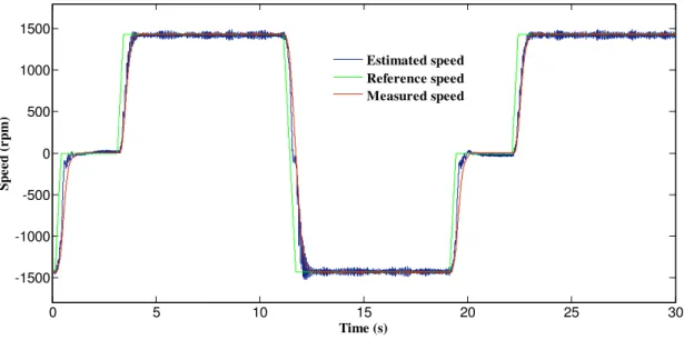
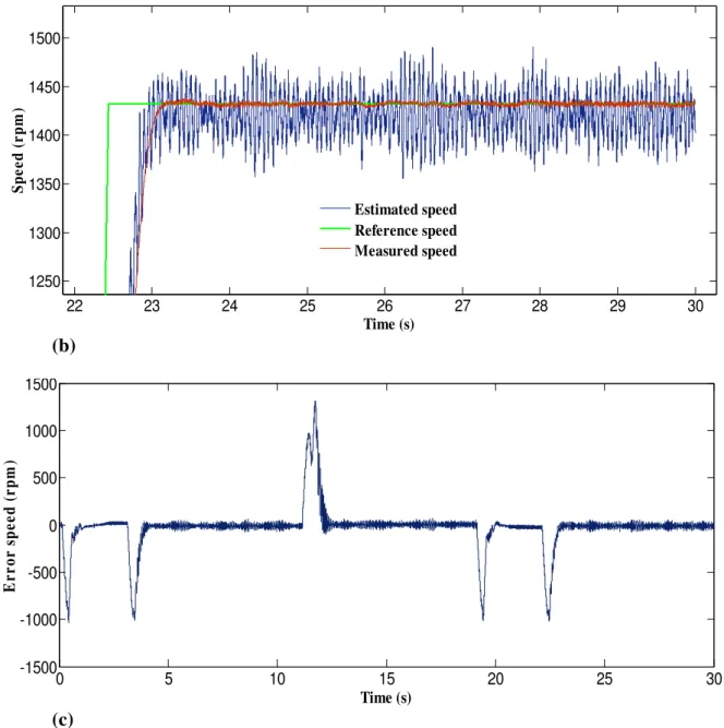
Scenario 3: Inversion of the speed

A step change in speed reference from +1490 rpm to -100% is applied at 11 sec. This

step change is equivalent to 100% speed change. The response is shown in figure 5. The

phase sequence reverses to rotate the motor in reverse direction. The drive reaches

steady-state for this change very short time. This proves that the speed estimation is stable even at

very low and zero speeds.

0 5 10 15 20 25 30

-1500 -1000 -500 0 500 1000 1500

Time (s)

Spe

e

d (

r

pm

)

(a)

(11)

22 23 24 25 26 27 28 29 30 1250

1300 1350 1400 1450 1500

Time (s)

Sp

e

d

(

r

pm

)

(b)

0 5 10 15 20 25 30

-1500 -1000 -500 0 500 1000 1500

Time (s)

E

r

ro

r

s

p

eed

(

r

p

m

)

(c)

Figure 5. Response of the drive at speed reversal with no load condition: (b) = Zoom of speed; (c) = Error of estimated speed

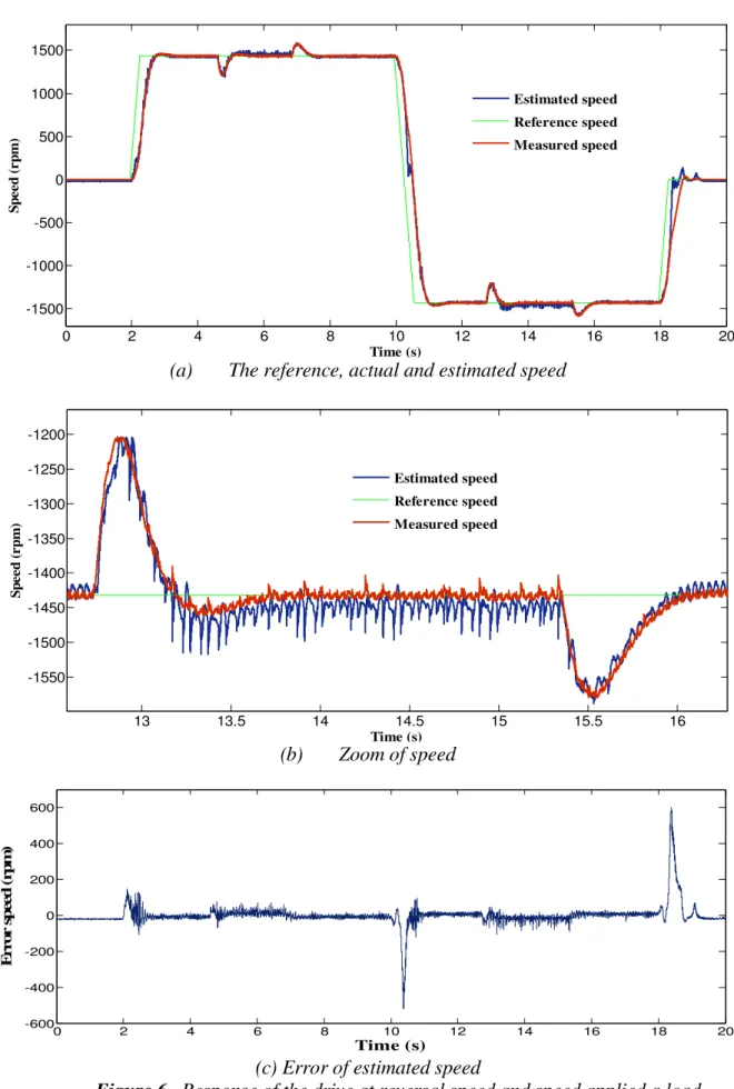
Scenario 4 Inversion of the speed under load change

In this scenario, the controller was tested under the speed dependent load produced by

the synchronous machine. The reversal speed response of the motor is shown in figure 6 at

high speeds under different levels of load torque. This figure indicates that the estimated

value also tracks its true value very closely in both the forward and reverse directions, and it

is possible to verify the excellent behaviour of the proposed algorithm. In fact, the waveforms

(12)

0 2 4 6 8 10 12 14 16 18 20 -1500

-1000 -500 0 500 1000 1500

Time (s)

Sp

e

d (

r

pm)

(a) The reference, actual and estimated speed

13 13.5 14 14.5 15 15.5 16

-1550 -1500 -1450 -1400 -1350 -1300 -1250 -1200

Time (s)

Sp

e

d

(

r

pm)

(b) Zoom of speed

0 2 4 6 8 10 12 14 16 18 20

-600 -400 -200 0 200 400 600

Time (s)

E

r

ro

r s

p

eed

(

rp

m

)

(c) Error of estimated speed

(13)

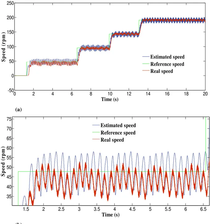
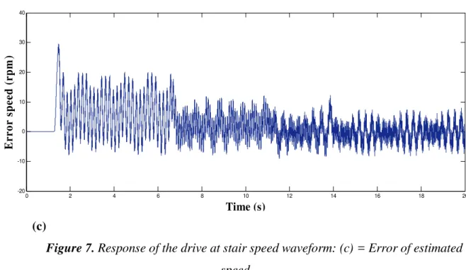
Scenario 5: Staircase tracking waveform include low speed region

A reference speed of 50 rpm was initially applied at t = 1.5 seconds, increased to 100

rpm, 150 rpm and 200 rpm respectively at t = 6.5 seconds, t=10 seconds and at t=13 seconds

(figure 7) (different level of speed including low speed region).

0 2 4 6 8 10 12 14 16 18 20

-50 0 50 100 150 200 250

Time (s)

Sp

e

d (

r

p

m

)

Estimated speed Reference speed Real speed

(a)

1.5 2 2.5 3 3.5 4 4.5 5 5.5 6 6.5

35 40 45 50 55 60 65 70 75

Time (s)

Spe

e

d (

r

p

m

)

Estimated speed Reference speed Real speed

(b)

(14)

0 2 4 6 8 10 12 14 16 18 20 -20

-10 0 10 20 30 40

Time (s)

E

rro

r s

p

ee

d

(

rp

m

)

(c)

Figure 7. Response of the drive at stair speed waveform: (c) = Error of estimated speed

It is seen that the speed responses were smooth in different speed zones. We can see

that the speed follow perfectly the speed reference. We note that the performance degrades as

approaching the low speed region and fails to provide small oscillations.

Conclusions

Both observers presented in the paper can estimate the speed in an electrical drive

system. The values of the on-line speed estimated can be used by the control of the electrical

drive systems in speed range. The main features are the following:

• The rotor speed of the motor is estimated by reference model with Luenberger observers.

• To obtain a high-dynamic current sensorless control, a current to voltage feed forward

decoupling and a good dynamic correction are obtained.

• Moreover, an accurate dynamic limitation of the real electromagnetic torque is obtained.

• The final algorithm can be implemented with relatively few instructions using the Embedded Matlab function block based on an M-file written in the MATLAB language

because it can be supported by RTI (Real Time Interface) with execution times of each

(15)

• Results of the dynamic and steady state behavior of a sensorless speed control of an

induction motor are given.

• The experimental results were satisfactory.

• Both at low, at load applied, at high and reversal motor speed the proposed control

scheme is working very well and proves a robustness of the proposed control structure in

dSPACE environment.

• The described control system is a solution without mechanical sensors for a wide range of applications where good steady state and dynamic properties are required.

At present, sensor-based controls are still widely used in industrial and transportation

applications. But in the near future, speed sensorless-based drive systems will become a

practical reality and will be used in many industrial applications. Sensorless-based systems

will provide higher reliability and operation in adverse environmental conditions at a lower

cost.

References

1. Mabrouk J., Jarray K., Koubaa Y., Boussak M.; A Luenberger State Observer for Simultaneous Estimation of Speed and Rotor Resistance in sensorless Indirect Stator Flux Orientation Control of Induction Motor Drive, IJCSI International Journal of Computer Science Issues, 2011, 6(8), 3 p. 116-125.

2. Ben Hamed M., Sbita L., Abboud W.; ANN Speed Sensorless Fuzzy Control of DRFOC Induction Motor Drives. Leonardo Electronic Journal of Practices and Technologies, 2010, 16, p. 129-150.

3. Piciu M.A., Comparison between Luenberger observer and Gopinath observer used in electrical drives systems without sensorless, 6th international conference on electromechanical and power systems, Rep.Moldova, 2007, p.51-54.

(16)

three-phase induction motors based on sliding mode for washing-machine drive applications. IEEE Trans. Ind. Appli., 2006, 42, p. 694-701.

6. Piciu M.A., Alboteanu L.., Sensorless Speed Control Systems Based on Adaptive Observers Luenberger and Gopinath, Annals of the University of Craiova, Electrical Engineering series, ISSN 1842-4805, 2008, 32, p. 124-129.

7. Kojabadi H.M., Simulation and experimental studies of model reference adaptive system for sensorless induction motor drive, Department of Electrical Engineering, 2005, 13 (6), p. 451-464.

8. Sbita L., Ben Hamed M., A MRAS-based speed estimation for a direct vector-controlled speed sensorless induction motor drives, Proceeding of the 4th IEEE International Conference on Systems, Signals and Devices, Hammamet, Tunisia, 2007.