Aerodynamic roughness length estimation from very high-resolution imaging LIDAR observations over the Heihe basin in China

(1)

HESSD

7, 3397–3421, 2010

Aerodynamic roughness length

estimation

J. Colin et al.

Title Page

Abstract Introduction

Conclusions References

Tables Figures

◭ ◮

Back Close

Full Screen / Esc

Printer-friendly Version Interactive Discussion

Discussion

P

a

per

|

Dis

cussion

P

a

per

|

Discussion

P

a

per

|

Discussio

n

P

a

per

|

Hydrol. Earth Syst. Sci. Discuss., 7, 3397–3421, 2010 www.hydrol-earth-syst-sci-discuss.net/7/3397/2010/ doi:10.5194/hessd-7-3397-2010

Hydrology and Earth System Sciences Discussions

This discussion paper is/has been under review for the journal Hydrology and Earth System Sciences (HESS). Please refer to the corresponding final paper in HESS if available.

Aerodynamic roughness length

estimation from very high-resolution

imaging LIDAR observations over the

Heihe basin in China

J. Colin1, R. Faivre1, and M. Menenti2

1

Image Sciences, Computing Sciences and Remote Sensing Laboratory, UMR7005 CNRS, University of Strasbourg, BP10413, 67412 ILLKIRCH Cedex, France

2

Faculty of Aerospace Engineering, Delft University of Technology, Kluyverweg 1, 2629HS, Delft, The Netherlands

Received: 8 April 2010 – Accepted: 27 April 2010 – Published: 8 June 2010 Correspondence to: J. Colin (j.colin@unistra.fr)

(2)

HESSD

7, 3397–3421, 2010

estimation

J. Colin et al.

Title Page

Tables Figures

◭ ◮

Back Close

Full Screen / Esc

Discussion

P

a

per

|

Dis

cussion

P

a

per

|

Discussion

P

a

per

|

Discussio

n

P

a

per

|

Abstract

Roughness length of land surfaces is an essential variable for the parameterisation of momentum and heat exchanges. The growing interest about the estimation of the sur-face turbulent flux parameterisation from passive remote sensing lead to an increasing development of models, and the common use of simple semi-empirical formulations 5

to estimate surface roughness. Over complex surface land cover, these approaches would benefit from the combined use of passive remote sensing and land surface struc-ture measurements from Light Detection And Ranging (LIDAR) techniques. Following early studies based on LIDAR profile data, this paper explores the use of imaging LI-DAR measurements for the estimation of the aerodynamic roughness length over a 10

heterogeneous landscape of the Heihe river basin, a typical inland river basin in the northwest of China. LIDAR points were used to extract a Digital Surface Model (DSM) and a Digital Elevation Model (DEM) from a single flight pass over an irrigated area covered by field crops, small trees arrays and tree hedges, with a ground resolution of 1 m and a total surface of 7.2 km2. As a first step, the DSM is used to estimate the 15

plan surface density and frontal surface density of obstacles to wind flow and compute a displacement height and roughness length following strictly geometrical approaches. In a second step, both the DSM and DEM are introduced in a Computational Fluid Dy-namics model (CFD) to calculate wind fields from the surface to the top of the Planetary Boundary Layer (PBL), and invert wind profiles for each calculation grid and compute 20

a roughness length. Examples of the use of these three approaches are presented for various wind direction together with a cross-comparison of results on heterogeneous land cover and complex roughness element structures.

1 Introduction

Roughness length (z0m) of land surfaces is an essential variable for the parameterisa-25

(3)

HESSD

7, 3397–3421, 2010

estimation

J. Colin et al.

Title Page

Tables Figures

◭ ◮

Back Close

Full Screen / Esc

Discussion

P

a

per

|

Dis

cussion

P

a

per

|

Discussion

P

a

per

|

Discussio

n

P

a

per

|

the surface energy balance components from passive remote sensing lead to a increas-ing development of models e.g. (Bastiaanssen et al., 1998; Roerink et al., 2000; Su, 2002; Colin et al., 2006b), some of which propose detailed parameterisation of resis-tances to heat transfer using advanced algorithm to retrieve roughness length for heat (z_0h) from kB−1 formulations (Massman, 1997; Bl ¨umel, 1999). However, as complex 5

as the parameterisation can be, the actual benefit from such formulations depends on an adequate estimate of the roughness length for momentum. Numerous formulations to derive this parameter fromNDVI can be found in many studies e.g. (Moran, 1990; Bastiaanssen, 1995), but are commonly used out of recommended bounds and on highly heterogeneous land surfaces, sometime leading to a significant degradation of 10

turbulent flux estimates (Colin et al., 2006a). These approaches would benefit from the combined use of passive remote sensing and land surface structure measurements from Light Detection And Ranging (LIDAR) techniques. Since the very early use of laser altimetry (Ketchum Jr., 1971), sensor performances have significantly improved, allowing airborne profiler to be used for surface aerodynamic roughness measurement 15

(Menenti and Ritchie, 1994). More recently, satellite and airborne imaging LIDAR sys-tems have paved the way to the mapping of vegetation properties over forest areas (Hofton et al., 2002), sometimes associated with complex topography (Dorren et al., 2007), but also on low vegetations like salt-marsh (Wang et al., 2009) or semi-arid steppe (Streutker and Glenn, 2006).

20

The objective of this paper is to explore the use of imaging LIDAR measurements for the estimation of the aerodynamic roughness length over a heterogeneous land-scape of the Heihe river basin, a typical inland river basin in the northwest of China. This investigation is part of the Watershed Allied Telemetry Experimental Research (WATER) project (Li et al., 2009), which is a simultaneous airborne, satellite-borne, 25

(4)

HESSD

7, 3397–3421, 2010

estimation

J. Colin et al.

Title Page

Tables Figures

◭ ◮

Back Close

Full Screen / Esc

Discussion

P

a

per

|

Dis

cussion

P

a

per

|

Discussion

P

a

per

|

Discussio

n

P

a

per

|

covered by field crops, small trees arrays and tree hedges, with a ground resolution of 1 m and a total surface of 7.2 km2. As a first step, the DSM is used to estimate the plan surface density and frontal surface density of obstacles to wind flow and compute a displacement height and roughness length following the work done by (Raupach, 1994) and (MacDonald et al., 1998). In a second step, both the DSM and DEM are 5

introduced in a Computational Fluid Dynamics model (CFD) to calculate wind fields from the surface to the top of the Planetary Boundary Layer (PBL), and invert wind profiles for each calculation grid and compute a roughness length. Examples of the use of these three approaches are presented for various wind direction together with a cross-comparison of results on heterogeneous land cover and complex roughness 10

element structures.

2 Theoretical background

The wind velocity profile over the land surface is commonly approximated by a simple logarithmic expression of the form:

u(z)= u_∗

k ·ln _z

−d0 z0m

(1) 15

where u_∗ is the friction velocity, k the von Karman constant, d0 the displacement height andz0m the aerodynamic roughness length. The later is usually expressed as a constant ratio of the canopy height for homogeneous surface like continuous low vegetation canopy, with a consensus for values of around z_0m

h_v≈0.1 (Brutsaert, 1982). However, the homogeneity assumption makes such kind of approximation of 20

(5)

HESSD

7, 3397–3421, 2010

estimation

J. Colin et al.

Title Page

Tables Figures

◭ ◮

Back Close

Full Screen / Esc

Discussion

P

a

per

|

Dis

cussion

P

a

per

|

Discussion

P

a

per

|

Discussio

n

P

a

per

|

(Lettau, 1969):

z0m=0.5·hv·λf (2)

were the frontal area index is defined as:

λf=

A_f AT

(3)

and expresses the ratio of frontal surfaceA_f (perpendicular to the flow) over the total 5

surface covered by roughness elements AT. A well-known formulation based on the

combined use ofhv and λf was then proposed in (Raupach, 1994). Here the frontal

area index is used in both the calculation ofd0 andz0m, leading to the formulation of the displacement height:

d0 h_v =1−

1−exp h

−(Cdl2λf)

0.5i

(Cdl2λf)0.5

(4) 10

and for the roughness length: z0m

h_v =

1−d0 h_v

·exp

−k_uU

∗

+ψ_h

(5)

with u_∗

U =min

(C_s+C_Rλ_f)0.5; _u

∗

U

max

(6)

whereψ_h expresses the influence of the roughness sublayer, C_s is the drag coeffi -15

cient for an obstacle free surface,C_R the drag coefficient for an isolated obstacle, and Cdl a free parameters. Recommended values of 0.193, 0.003, 0.3 and 7.5 a,

respec-tively used, as for u_∗ U

(6)

HESSD

7, 3397–3421, 2010

estimation

J. Colin et al.

Title Page

Tables Figures

◭ ◮

Back Close

Full Screen / Esc

Discussion

P

a

per

|

Dis

cussion

P

a

per

|

Discussion

P

a

per

|

Discussio

n

P

a

per

|

(Theurer, 1993) quoted in (MacDonald et al., 1998) noted thatz0m and d0 could be approached by combining the frontal area index with the plan area index defined as:

λ_p=Ap

A_T (7)

wereApis the plan surface of the roughness elements within the same total surface

A_T. The plan area indexλ_pis related to the importance of intervening spaces between 5

roughness elements. Considering an array of roughness elements of equivalent height, the canopy tends to be a homogeneous surface to airflow whenλptends to 1.

increas-ing the displacement height. This allows describincreas-ing the non-monotonic behaviour of z0m with λf. If the frontal area index is related to z0m, an increase of λp leads to a decrease of the drag e_ffect of the roughness elements. Therefore the Lettau’s formula-10

tion ofz0mis known to fail for plan area index higher than 0.2–0.25, because of mutual effects of high frontal area index and limited intervening spaces.

This was expressed by (MacDonald et al., 1998), who proposed two formulations forz0m andd0based on Lettau’s concept to account for a larger variety of geometrical configurations of roughness elements, and show an appropriate behaviour over the en-15

tire range of density indexes. The ratio of the displacement height over the roughness element height is expresses as:

d0

h_v =1+α

−λp _λ p−1

(8)

The convexity can be controlled byα. Experiments lead (MacDonald et al., 1998) to recommend a value ofα=4.43 for staggered arrays of roughness elements andα=3.59 20

for squared arrays. This ratio is then incorporated in the calculation of the ratio of the roughness length over the roughness element height following:

z₀_m h_v =

1−d0

h_v

exp "

−

0.5βCD k2

1−d0

h_v

λ_f

−0.5#

(7)

HESSD

7, 3397–3421, 2010

estimation

J. Colin et al.

Title Page

Tables Figures

◭ ◮

Back Close

Full Screen / Esc

Discussion

P

a

per

|

Dis

cussion

P

a

per

|

Discussion

P

a

per

|

Discussio

n

P

a

per

|

The expression includes the obstacle drag coefficient C_D=1.2, and an extra β co-e_fficient to best fit the relation with experiments. In the following study this coe_ffi -cient is not used (β=1). This formulation proved to reproduces the peak ofz0m

h_v for λ_f=0.15−0.30, which is consistent with wind tunnel experiments.

Beside the use of the plan area and frontal area index, the direct use of both the 5

DEM and DSM in a Computational Fluid Mechanics (CFD) solver is explored. The CFD solver called Canyon, embedded in the WindStation software (Lopes, 2003), al-lows for numerical simulations of turbulent fal-lows over complex topography, and can account for the geometry of surface roughness elements through the Digital Surface Model, as obtained from LIDAR data. The solver follows a control-volume approach, 10

and solves for mass conservation, momentum conservation following Navier-Stokes equations, and also energy conservation for non-neutral situations. 3-D wind fields ob-tained in output of the CFD express the combined effect of topography and roughness elements on the airflow, and result from the solving of the transport equation. Values of wind speed of a given profile not only characterise local effects of the vegetation 15

structure, but the total surface stress resulting from the upstream roughness elements on a distance called the length scale (Menenti and Ritchie, 1994). This length scale is usually considered to be of 1–2 order of magnitude of the height of the wind profile used for roughness length calculation. Therefore an aerodynamic roughness length can be obtained from the wind profile of each computation grid by inverting Eq. (1) with 20

values within the ground and a given elevation.

3 Experiment

3.1 Study area

The HeiHe River Basin is a typical inland river basin in the northwest of China. Sec-ond largest inland river basin of the country, it is located between 97◦₂₄′_–102◦₁₀′_E

25

(8)

Ex-HESSD

7, 3397–3421, 2010

estimation

J. Colin et al.

Title Page

Tables Figures

◭ ◮

Back Close

Full Screen / Esc

Discussion

P

a

per

|

Dis

cussion

P

a

per

|

Discussion

P

a

per

|

Discussio

n

P

a

per

|

periments conducted in the scope of the WATER project consisted in simultaneous airborne, satellite-borne and ground-based remote sensing measurements aiming at improving the observability, understanding and predictability of hydrological and eco-logical processes at catchment scale (Li et al., 2009). Observations focused on six dif-ferent areas with landscapes ranging from desert steppe and gobi desert to grassland 5

and irrigated farmland. Airborne data used in this study were acquired over the Yingke area. The Yingke Oasis, located to the south of Zhangye city (100◦25′E, 38◦51′N, 1519 m a.s.l.), is a typical irrigated farmland. The primary crops are maize and wheat, with fields often separated by tree hedges. This site was selected for its interest in in-vestigating crop evapotranspiration, bio-geophysical and structure parameters of crop, 10

interaction between groundwater and surface water, and irrigation.

3.2 Airborne LIDAR

The WATER field campaign has been completed with an intensive observation period. Twenty-five missions were flown in 2008 with different sensors. This study is based on the use of an LiteMapper 5600 imaging LIDAR, whose major characteristics are a 15

wavelength of 1550 nm, a pulse of 3.5 ns at 100 kHz and a scan angle range of±22.5◦. The spatial density for a flight height of 800 m above the ground is 4 impacts per square meter. After correction of the raw data to account for the attitude of the plane, point clouds are processes to extract of the minimum and maximum values for each square meter grid, providing a Digital Elevation Model and a Digital Surface Model respectively, 20

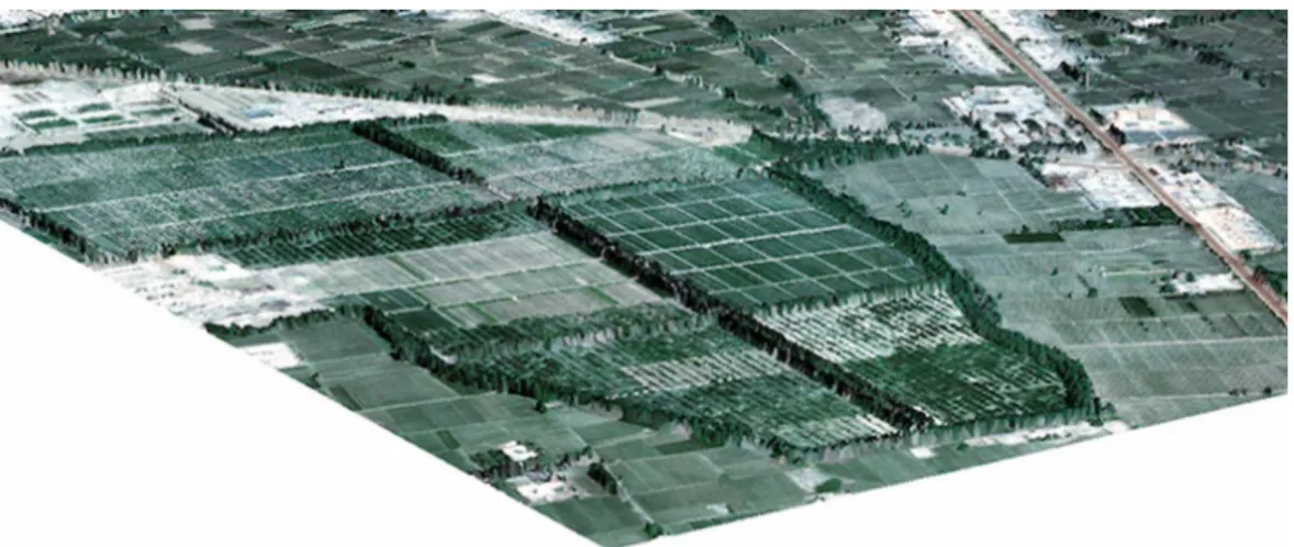
with a spatial resolution of 1 m. The LIDAR flight used here was operated the 20 June 2008, and the scene covers an area of 7.2 km2. A 3-D view of a subset of the entire dataset is presented in Fig. 2.

3.3 Meteorological data

The Yingke Oasis experimental site is permanently instrumented with an Automatic 25

(9)

HESSD

7, 3397–3421, 2010

estimation

J. Colin et al.

Title Page

Tables Figures

◭ ◮

Back Close

Full Screen / Esc

Discussion

P

a

per

|

Dis

cussion

P

a

per

|

Discussion

P

a

per

|

Discussio

n

P

a

per

|

at 2 and 10 m, and air pressure, relative humidity, precipitation, net radiation, soil heat flux, soil temperature and water content every ten minutes. Moreover, latent heat flux, sensible heat flux and water vapour concentration are obtained from eddy correlation systems with an integration step of 30 min.

Six atmospheric soundings were performed during June and July 2008 with GPS-5

tracking balloons. The instruments onboard have measured air temperature, relative humidity, air pressure, wind horizontal component and direction, mixing ratio and some information about localization and altitude.

3.4 Implementation of the approach from (MacDonald et al., 1998)

The canopy height obtained by difference between the DSM and DEM gives the distri-10

bution of roughness elements over the entire area. Considering a subset grid of this area with a surface AT, and the total surface of roughness elements Ap within this

subset, it is possible to compute a plan area index for the grid. The separation of pix-els between roughness element and intervening space was performed by defining a height threshold from the vertical distribution of pixels. It should be noted that a∆h≈0 15

within a LIDAR grid can either mean that there is no vegetation within this grid, or that the canopy if homogeneous and dense enough to prevent impulses to reach the soil underneath. In both cases it could be considered that this grid belongs to interven-ing spaces in between bigger roughness elements. In the followinterven-ing calculations, the threshold was defined as 12 cm. In the same way, pixels of the same subset grid of 20

surfaceA_T can be projected on a plan surface orthogonal to the airflow, giving a total integrated surfaceAf used to compute the frontal area index.

A tool was developed for these purposes. Considering a given grid size, a number of wind direction (2, 4, 8. . . ) and an input pixel size, the tool will sequentially compute the plan area index, the frontal area indexes for each wind directions, and the asso-25

(10)

HESSD

7, 3397–3421, 2010

estimation

J. Colin et al.

Title Page

Tables Figures

◭ ◮

Back Close

Full Screen / Esc

Discussion

P

a

per

|

Dis

cussion

P

a

per

|

Discussion

P

a

per

|

Discussio

n

P

a

per

|

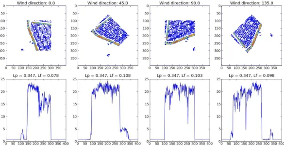
view within a grid, as illustrated in Fig. 3.

Depending of wind direction, the shape of the frontal surface opposed to wind flow can change significantly, as illustrated on Fig. 3, with frontal area index ranging from 0.078 to 0.108. In this particular example, the effect of the orientation of the airflow as compared to the orientation of the tree hedges explains most of the variation, with high 5

values when the wind is perpendicular to the wind flow (45◦and 90◦), and lower ones when it becomes nearly parallel (0◦and 135◦).

3.5 Configuration of the computational fluid dynamics model

The Canyon CFD requires the input of a Digital Elevation Model and at least one local set of wind profile properties for initialization, i.e. wind speed and direction at two lev-10

els, and the height of the top of the Planetary Boundary Layer. It can use a roughness element height map whenever available, or assumes this height constant on the entire scene. In this study, the Digital Surface Model is used to document the height of the elements on the entire scene. Therefore model can account for both the topography and the surface stress from roughness elements. It should be noted that the Yingke 15

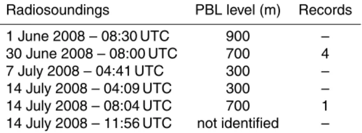
area is almost planar, with a very slight slope from West to East leading to an altitude difference of nearly 30 m over the 2400 m swath of the LIDAR path. The AWS wind speed and direction measurements at 2 and 10 m are used to initialize the profile, to-gether with the PBL height obtained from nearly simultaneous atmospheric soundings (Table 1). In the following experiments, meteorological contexts are limited to neutrally 20

(11)

HESSD

7, 3397–3421, 2010

estimation

J. Colin et al.

Title Page

Tables Figures

◭ ◮

Back Close

Full Screen / Esc

Discussion

P

a

per

|

Dis

cussion

P

a

per

|

Discussion

P

a

per

|

Discussio

n

P

a

per

|

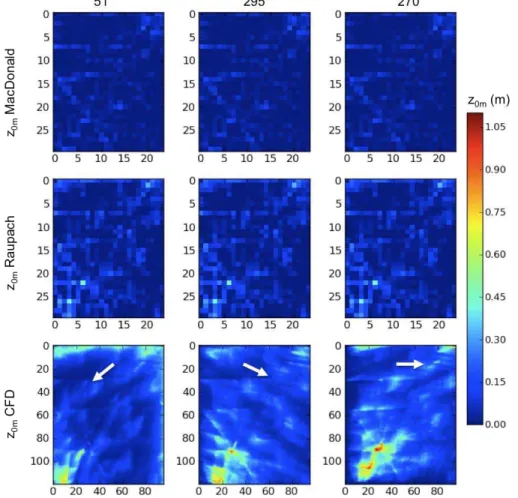
4 Results and discussion

4.1 Wind field computation

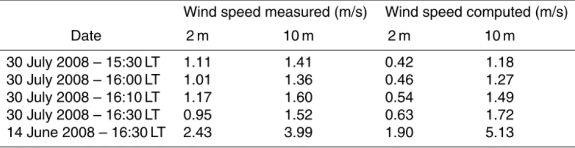
Wind fields were computed with a ground resolution of 25 m and 15 levels from 5 to 870 m above ground. A control of the computed wind speed at 2 and 10 m with original values from the AWS reveals that speeds can significantly vary. Table 3 shows 5

di_fferences between measured and simulated wind speed values. The di_fferences are more important near the surface, with a mean underestimation of 40% for CFD wind speeds at 2m, but reduce at 10 m, with a mean underestimation of 10% and mean overestimation of 20%. As quoted in Sect. 2, this is due to the solving of the transport equation.

10

Output wind fields are affected by a border effect on the upstream boundaries of the scene (e.g. on the lower left image of Fig. 4). This imposes to discard results within the first 150 m north and east of the fields. It could however be overcome following a nested scale approach, with use of a lower resolution regional DEM to compute a first initialization field to be used in place of the AWS initialization measurements. This 15

couldn’t be performed at this stage of the study.

4.2 Roughness length processing

LIDAR data were processed to compute the plan area index of the scene, the frontal area indexes for each wind directions, and associated displacement height following both the approaches from Raupach and MacDonald. The average height of roughness 20

elements within the scene lead to choose a grid size of 100 m, i.e. ten times the height of most of the obstacles to airflow, also tree hedges usually reach 30 m, and up to 38 m for some trees. However, the following calculations stick to the 100 m grid to preserve some granularity. Values ofλ_pwere found to range between 0.08 to 0.64 for tree arrays and some building groups. This leads tod0(Raupach)/hv values mainly ranging between

25

(12)

HESSD

7, 3397–3421, 2010

estimation

J. Colin et al.

Title Page

Tables Figures

◭ ◮

Back Close

Full Screen / Esc

Discussion

P

a

per

|

Dis

cussion

P

a

per

|

Discussion

P

a

per

|

Discussio

n

P

a

per

|

for dense low tree arrays. The lowest λ_f values are of 0.025, but can reach 0.2 for grids containing tree hedges. These values are globally rather low because the area doesn’t contain regular arrays of high elements, but rather one-line obstacles like the alignments of trees. Values ofz0m are very similar from one orientation to the other, e.g. with a variation of the order of±8.10−3m between values obtained with a 51◦and 5

270◦airflow. However, signification variations with wind direction in frontal area index, and as a consequence in roughness length, can be obtained for grids containing tree line structures, as illustrated on Fig. 3. The difference of values of z0m between the formulations of Raupach and MacDonald are more significant, and a related to the larger values of displacement height obtained over densely vegetated surface from the 10

MacDonald’s formulation. Indeed,z0m(Raupach)range from 0.015 to nearly 0.51. with a maximumz0m(Raupach)/hv of 0.142, whilez0m(MacDonald)from 0.015 to 0.195, maximum z0m(MacDonald)/hv of 0.120.

CFD based roughness obtained from the inversion of Eq. (1) using wind fields give a rather different view of the surface drag effect. Also computations are made at a 25 m 15

ground resolution, a grid values expresses the effect of surface stress upstream on the entire footprint of the profile used in the inversion, while the geometrical approach can only account for the frontal density of obstacles within the calculation grid. Here it is assumed that the footprint for the selected neutral conditions is ten times the height of the profile. To obtain results at local scale, the wind field levels from the ground up 20

to 30 m are used to compute the roughness length, for an assumed footprint size of 300 m. Results presented in Fig. 4 illustrate very well in particular the shelter effect of tree hedges, and simulations differ significantly from one wind direction to the other. Here z0m values are of the order of 0.02–0.03 for low vegetation areas, 0.12–0.2 for corn fields, but can reach values as high as 0.8 and even 1.1 nearby tree hedges 25

(13)

HESSD

7, 3397–3421, 2010

estimation

J. Colin et al.

Title Page

Tables Figures

◭ ◮

Back Close

Full Screen / Esc

Discussion

P

a

per

|

Dis

cussion

P

a

per

|

Discussion

P

a

per

|

Discussio

n

P

a

per

|

4.3 Discussion

A strict grid per grid comparison between geometrical and CFD based results may not be relevant. Indeed geometrical approaches account for airflow orientation, but they cannot reproduce the footprint e_ffect of upstream roughness elements. These approaches are designed for regular arrays of roughness elements. It can very well 5

account for heterogeneity in terms of e.g. grassland with staggered arrays of trees, or any configuration where local heterogeneity tends to a meso-scale homogeneity. However, in such a complex land cover context, the CFD approach proves to give a much finer view of interactions between the airflow and the structure and orientations of roughness elements of significant height. That said, geometrical and CFD basedz0m 10

tend to converge on large, open areas covered either by bare soil, grassland, low field crops, and even to some extend on some corn fields. For an example, Fig. 5b shows in green output grids wherez0m(Raupach) matchz0m(CFD) within an interval of±0.05 m. Compared to the Digital Surface Model presented on Fig. 5a, and considering that the wind direction is 51◦, it appears rather clearly that beside areas affected by a significant 15

shelter effects, both approach tend to give comparable results. This suggests that geometrical formulation could give more comparable results on natural heterogeneous land covers present in the region, like the sparse grassland and low trees land covers. It should be mentioned that the values obtained from the CFD wind fields for grids containing tall trees might not be correct. In these calculations, it was decided to use 20

the levels of wind fields within the first 30 m to stick to the 300 m footprint, also in some areas some trees can reach up to 38 m. Further investigations are needed to check the quality of the wind speed estimates in the lower part of the boundary, but it seems clear that in cases were roughness elements can reach such a height, the footprint size should be reconsidered, e.g. by using the first 60 m of wind profiles.

25

(14)

HESSD

7, 3397–3421, 2010

estimation

J. Colin et al.

Title Page

Tables Figures

◭ ◮

Back Close

Full Screen / Esc

Discussion

P

a

per

|

Dis

cussion

P

a

per

|

Discussion

P

a

per

|

Discussio

n

P

a

per

|

computation of the frontal area index cannot account for a more significant variation of the elevation, while the combined use of the DEM and DSM in the CFD could still give consistent results.

Finally, it must be emphasised that both the geometrical and CFD approaches as-sume roughness elements to be solid blocks. In both cases, the Digital Surface Model 5

is used to derive an obstacle height that is used either to estimate a frontal surface and intervening spaces, or as a first assumption on local roughness. But none of these approaches will account for the porosity of vegetation structures. In particular, it is obvious that such a representation of obstacles like the tree hedges will lead to over-estimate their effect on the flow, while these trees will mainly oppose a resistance to 10

the airflow on levels with the highest foliage density. Therefore, the computation of the roughness length over complex land cover would require accounting for the vertical structure of the canopy. This could be achieved by use of the full waveform of the LI-DAR measurements, instead of the use of statistics on points used here. Also the full waveform was retrieved during LIDAR acquisition over the Yingke oasis, these dataset 15

still require further pre-processing, and couldn’t be exploited in this study.

5 Conclusion and perspectives

Hydrological and micro-meteorological studies based on the modelling of surface heat exchanges from radiometric observations can benefit from the contribution of very high-resolution LIDAR digital elevation and digital surface models over a complex land cover. 20

The geometrical characterisation of the surface topography but also the structure of the roughness elements paves the way for a more accurate modelling of aerodynamic processes, and in particular a detailed estimate of the surface roughness. The im-plementation of the geometrical approaches to compute the plan area index and the frontal area index, together with the formulations from Raupach and MacDonald in a 25

(15)

HESSD

7, 3397–3421, 2010

estimation

J. Colin et al.

Title Page

Tables Figures

◭ ◮

Back Close

Full Screen / Esc

Discussion

P

a

per

|

Dis

cussion

P

a

per

|

Discussion

P

a

per

|

Discussio

n

P

a

per

|

scale. On the other hand, the combined used of the DEM and the DSM in a CFD model proves to account for the complexity of the land cover, in particular for staggered structures of tall roughness elements. However, the spatial meaning of the values is different from the gridded geometrical approaches, as a 25 m resolution grid actually accounts for the upstream surface stress within its own footprint. It is also emphasized 5

that both the geometrical and CFD based approach rely on a simple representation of the roughness elements, and do no account for the porosity of foliage structures to the airflow. The definition of the exact footprint of such computations still needs to be investigated. And a cross comparison of results from the CFD based approach with ground measurements at footprint scale could provide a first validation of the results. 10

Moreover, a general analysis of the structure of the landscape along the airflow should allow for an adequate definition of the footprint size and related wind fields levels to be used in the inversion. Results would also benefit from a nested scale computation of the wind fields. The use of coarser DEM over a larger area for the initialization of the high-resolution computations should remove any border effects. Finally, the use of 15

such approaches over other land cover types, but also more accentuated topographies within the Heihe basin could give an extended view of the adequacy of both approaches is various contexts.

Acknowledgements. This study is supported by the ESA Dragon II program under proposal no. 5322: “Key Eco-Hydrological Parameters Retrieval and Land Data Assimilation System

20

Development in a Typical Inland River Basin of China’s Arid Region” and by the European Commission (Call FP7-ENV-2007-1 Grant nr. 212921) as part of the CEOP-AEGIS project (http: //www.ceop-aegis.org) coordinated by the University of Strasbourg. WATER is jointly supported by the Chinese Academy of Science Action Plan for West Development Program (grant KZCX2-XB2-09) and Chinese State Key Basic Research Project (grant 2007CB714400). The authors

25

(16)

HESSD

7, 3397–3421, 2010

estimation

J. Colin et al.

Title Page

Tables Figures

◭ ◮

Back Close

Full Screen / Esc

Discussion

P

a

per

|

Dis

cussion

P

a

per

|

Discussion

P

a

per

|

Discussio

n

P

a

per

|

References

Bastiaanssen, W.: Regionalization of surface flux densities and moisture indicators incomposite terrain: a remote sensing approach under clear skies in Mediterranean climates, PhD thesis, University of Wageningen, 273 pp., 1995.

Bastiaanssen, W., Menenti, M., Feddes, R., and Holtslag, A. A. M.: A remote sensing surface

5

energy balance algorithm for land (SEBAL), 1. Formulation, J. Hydrol., 212–213, 198-212, 1998.

Bl ¨umel, K. B.: A simple formula for estimation of the roughness length for heat transfer over partly vegetated surfaces, J. Appl. Meteorol., 38, 814–829, 1999.

Brutsaert, W.: Evaporation into the atmosphere, Springer, London, 814–829, 1982.

10

Colin, J., Menenti, M., Rubio, E., and Jochum, A.: Accuracy Vs. Operability: a case study over Barrax in the context of the DEMETER project, AIP Conf. Proc., 852, 75–83, 2006.

Colin, J., Menenti, M., Rubio, E., and Jochum, A.: A Multi-Scales Surface Energy Balance System for operational actual surface evapotranspiration, AIP Conf. Proc., 852, 178–184, 2006.

15

Counehan, J.: Wind tunnel determination of the roughness length as a function of the fetch and the roughness density of three-dimensional roughness elements, Atmos. Environ., (1967), 5(8), 637–642, 1971.

Dorren, L., Berger, F., and Maier, B.: Mapping the structure of forestal vegetation with an air-borne light detection and ranging (LiDAR) system in mountainous terrain (Cartographier la

20

structure de la vegetation forestiere avec un systeme LiDAR a éroport é en terrain montag-nard), Revue Francaise de Photogrammetrie et de T él éd étection, (186), 54–59, 2007. Hofton, M. A., Rocchio, L. E., Blair, J. B., and Dubayah, R.: Validation of Vegetation Canopy

Lidar sub-canopy topography measurements for a dense tropical forest, J. Geodyn., 34(3–4), 491–502, 2002.

25

Ketchum Jr., R. D.: Airborne laser profiling of the arctic pack ice, Remote Sens. Environ., 2(C), 41–52, 1971.

Lettau, H.: Note on aerodynamic parameter estimation on the basis of roughness-element description, J. Appl. Meteorol., 8(5), 828–832, 1969.

Li, X., Li, X., Li, Z., Ma, M., Wang, J., Xiao, Q., Liu, Q., Che, T., Chen, E., Yan, G., Hu, Z.,

30

(17)

HESSD

7, 3397–3421, 2010

estimation

J. Colin et al.

Title Page

Tables Figures

◭ ◮

Back Close

Full Screen / Esc

Discussion

P

a

per

|

Dis

cussion

P

a

per

|

Discussion

P

a

per

|

Discussio

n

P

a

per

|

Res., 114, D22103, doi:10.1029/2008JD011590, 2009.

Lopes, A. M. G.: Windstation – A software for the simulation of atmospheric flows over complex topography, Environ. Modell. Softw., 18(1), 81–96, 2003.

MacDonald, R. W., Griffiths, R. F., and Hall, D. J.: An improved method for the estimation of surface roughness of obstacle arrays, Atmos. Environ., 32(11), 1857–1864, 1998.

5

Massman, W. J.: An analytical one-dimensional model of momentum transfer by vegetation of arbitrary structure, Bound.-Lay. Meteorol., 83, 407–421. 1997.

Menenti, M. and Ritchie, J. C.: Estimation of effective aerodynamic roughness of Walnet Gulch watershed with laser altimeter measurements, Water Ressources Research, (5), 1329–37, 1994.

10

Moran, M. S.: A satellite-based approach for evaluation of the spatial distribution of evapotran-spiration from agricultural lands, PhD thesis, University of Arizona, 223 pp., 1990.

Raupach, M. R.: Simplified expressions for vegetation roughness length and zero-plane dis-placement as functions of canopy height and area index, Bound.-Lay. Meteorol., 71(1–2), 211–216, 1994.

15

Roerink, G., Su, Z., and Menenti, M.: S-SEBI: A simple remote sensing algorithm to estimate the surface energy balance, Phys. Chem. Earth., 25(2), 147–157, 2000.

Streutker, D. R. and Glenn, N. R.: LiDAR measurement of sagebrush steppe vegetation heights, Remote Sens. Environ., 102(1–2), 135–145, 2006.

Su, Z.: The Surface Energy Balance System (SEBS) for estimation of turbulent heat fluxes,

20

Hydrol. Earth Syst. Sci., 6, 85–100. doi:10.5194/hess-6-85-2002, 2002.

Theurer, W.: Dispersion of Ground-Level Emissions in Complex Built-up Areas, Doctoral The-sis, Department of Architecture, University of Karlsruhe, Germany, 1993.

Wang, C., Menenti, M., Stoll, M. P., Feola, A., Belluco, E., and Marani, M.: Separation of ground and low vegetation signatures in LiDAR measurements of salt-marsh environments, IEEE T.

25

Geosci. Remote., 47(7), 2014–2023, 2009.

(18)

HESSD

7, 3397–3421, 2010

estimation

J. Colin et al.

Title Page

Tables Figures

◭ ◮

Back Close

Full Screen / Esc

Discussion

P

a

per

|

Dis

cussion

P

a

per

|

Discussion

P

a

per

|

Discussio

n

P

a

per

|

Table 1.PBL level and number of AWS records associated to atmospheric soundings.

(19)

HESSD

7, 3397–3421, 2010

estimation

J. Colin et al.

Title Page

Tables Figures

◭ ◮

Back Close

Full Screen / Esc

Discussion

P

a

per

|

Dis

cussion

P

a

per

|

Discussion

P

a

per

|

Discussio

n

P

a

per

|

Table 2.Wind speed and direction measured at Yingke AWS for the selected neutrally stratified

PBL conditions.

Wind speed (m/s)

(20)

HESSD

7, 3397–3421, 2010

estimation

J. Colin et al.

Title Page

Tables Figures

◭ ◮

Back Close

Full Screen / Esc

Discussion

P

a

per

|

Dis

cussion

P

a

per

|

Discussion

P

a

per

|

Discussio

n

P

a

per

|

Table 3.Comparison between measured and simulated wind speed values.

Wind speed measured (m/s) Wind speed computed (m/s)

Date 2 m 10 m 2 m 10 m

(21)

HESSD

7, 3397–3421, 2010

estimation

J. Colin et al.

Title Page

Tables Figures

◭ ◮

Back Close

Full Screen / Esc

Discussion

P

a

per

|

Dis

cussion

P

a

per

|

Discussion

P

a

per

|

Discussio

n

P

a

per

|

Fig. 1.(top left) location of the HeiHe River Basin in the Popular Republic China; (right) location

(22)

HESSD

7, 3397–3421, 2010

estimation

J. Colin et al.

Title Page

Tables Figures

◭ ◮

Back Close

Full Screen / Esc

Discussion

P

a

per

|

Dis

cussion

P

a

per

|

Discussion

P

a

per

|

Discussio

n

P

a

per

|

Fig. 2. Example of 3-D rendering of the South-West part of the Yingke area obtained by

(23)

HESSD

7, 3397–3421, 2010

estimation

J. Colin et al.

Title Page

Tables Figures

◭ ◮

Back Close

Full Screen / Esc

Discussion

P

a

per

|

Dis

cussion

P

a

per

|

Discussion

P

a

per

|

Discussio

n

P

a

per

|

Fig. 3. example of frontal profiles for a 100 m grid containing field crops and tree hedges,

(24)

HESSD

7, 3397–3421, 2010

estimation

J. Colin et al.

Title Page

Tables Figures

◭ ◮

Back Close

Full Screen / Esc

Discussion

P

a

per

|

Dis

cussion

P

a

per

|

Discussion

P

a

per

|

Discussio

n

P

a

per

|

Fig. 4.Roughness length maps derived from the LIDAR data over the Yingke area for 441 wind

(25)

HESSD

7, 3397–3421, 2010

estimation

J. Colin et al.

Title Page

Tables Figures

◭ ◮

Back Close

Full Screen / Esc

Discussion

P

a

per

|

Dis

cussion

P

a

per

|

Discussion

P

a

per

|

Discussio

n

P

a

per

|

Fig. 5. (a)Roughness element height from the DSM (in m);(b)areas where bothz_0m(Raupach)