Comparison of satellite microwave backscattering (ASCAT) and visible/near-infrared reflectances (PARASOL) for the estimation of aeolian aerodynamic roughness length in arid and semi-arid regions

(1)

AMTD

5, 2933–2957, 2012

Aeolian roughness length

C. Prigent et al.

Title Page

Abstract Introduction

Conclusions References

Tables Figures

◭ ◮

Back Close

Full Screen / Esc

Printer-friendly Version Interactive Discussion

Discussion

P

a

per

|

Dis

cussion

P

a

per

|

Discussion

P

a

per

|

Discussio

n

P

a

per

|

Atmos. Meas. Tech. Discuss., 5, 2933–2957, 2012 www.atmos-meas-tech-discuss.net/5/2933/2012/ doi:10.5194/amtd-5-2933-2012

Atmospheric Measurement Techniques Discussions

This discussion paper is/has been under review for the journal Atmospheric Measurement Techniques (AMT). Please refer to the corresponding final paper in AMT if available.

Comparison of satellite microwave

backscattering (ASCAT) and

visible/near-infrared reflectances

(PARASOL) for the estimation of aeolian

aerodynamic roughness length in arid

and semi-arid regions

C. Prigent, C. Jim ´enez, and J. Catherinot

Laboratoire d’Etudes du Rayonnement et de la Mati `ere en Astrophysique (LERMA), UMR8112, CNRS, Observatoire de Paris, France

Received: 6 February 2012 – Accepted: 23 March 2012 – Published: 17 April 2012 Correspondence to: C. Prigent ([email protected])

(2)

AMTD

5, 2933–2957, 2012

C. Prigent et al.

Title Page

Tables Figures

◭ ◮

Back Close

Full Screen / Esc

Discussion

P

a

per

|

Dis

cussion

P

a

per

|

Discussion

P

a

per

|

Discussio

n

P

a

per

|

Abstract

Previous studies examined the possibility to estimate the aeolian aerodynamic rough-ness length from satellites, either from visible/near-infrared observations or from mi-crowave backscattering measurements. Here we compare the potential of the two approaches and propose to merge the two sources of information to benefit from

5

their complementary aspects, i.e. the high spatial resolution of the visible/near-infrared (PARASOL part of the A-Train) and the independence from atmospheric contamina-tion of the active microwaves (ASCAT on board MetOp). A global map of the aeolian aerodynamic roughness length at 6 km resolution is derived, for arid and semi-arid re-gions. It shows very good consistency with the existing information on the properties of

10

these surfaces. The dataset is available to the community, for use in atmospheric dust transport models.

1 Introduction

Aeolian aerodynamic roughness length in arid regions is a key parameter to predict the vulnerability of the surface to wind erosion, and, as a consequence, the related

pro-15

duction of mineral aerosol (e.g. Raupach et al., 1993; Marticorena et al., 1995, 1997; Tegen et al., 2000; Shao, 2001; Laurent et al., 2008; Todd et al., 2008). Aerodynamic roughness length is defined as the height where the wind speed becomes zero, assum-ing a logarithmic wind profile. It affects both the quantity of potentially eroded material and the minimum wind speed required to raise the dust particles (Gillette and Passi,

20

1988). Physical models of mineral dust emissions have thus been developed based on an explicit description of the main physical processes involved during dust produc-tion (e.g. Marticorena and Bergametti, 1995; Shao, 2001; Alfaro and Gomes, 2001). They include parameterizations of the erosion threshold as a function of the surface roughness parameters. However, the use of such physical models are limited by the

25

(3)

AMTD

5, 2933–2957, 2012

C. Prigent et al.

Title Page

Tables Figures

◭ ◮

Back Close

Full Screen / Esc

Discussion

P

a

per

|

Dis

cussion

P

a

per

|

Discussion

P

a

per

|

Discussio

n

P

a

per

|

areas, especially their aerodynamic roughness length (Laurent et al., 2008; Darmen-ova et al., 2009). Recent dust model intercomparisons (e.g. Uno et al., 2006; Todd et al., 2008; Darmenova et al., 2009) emphasize the need for improved dust emission modeling, along with their key input parameters, including the roughness parameters, to accurately quantify the role of mineral aerosol in a changing climate. Note that the

5

dust emission scheme requires parameters at spatial and temporal scales relevant to dust emission: the aerodynamic roughness length used by regional and global land surface models are not relevant to the dust emission processes (Darmenova et al., 2009).

The aeolian roughness length is difficult to estimate, even locally. In situ

measure-10

ments usually consist in measuring the wind velocity profile from several anemome-ters on a mast, in near-neutral stability conditions (e.g. Greeley et al., 1997; MacKin-non et al., 2004). Marticorena et al. (1997) and Callot et al. (2000) developed maps of aerodynamic roughness length for North Africa and the Middle East, based on a geomorphological approach that combines topographic data, geological information,

15

aerial pictures, and in situ observations. Satellite observations are an effective solu-tion for a global homogeneous and systematic monitoring of the arid and semi-arid regions. Radar observations are sensitive to surface roughness, among other param-eters. Greeley et al. (1997) demonstrated a high correlation betweenz0 and the radar

backscattering using observations from aircraft and from the Shuttle Radar Laboratory

20

at 1.4 and 5.25 GHz in coincidence with field measurements. More recently, Prigent et al. (2005) derived global maps of aerodynamic roughness lengths in arid and semi-arid regions from the scatterometer measurements on board ERS. The estimates are provided with a spatial resolution of 0.25◦

×0.25◦, on a monthly basis. The scatterometer spatial resolution is limited (50 km) but the observations are almost insensitive to

atmo-25

(4)

AMTD

5, 2933–2957, 2012

C. Prigent et al.

Title Page

Tables Figures

◭ ◮

Back Close

Full Screen / Esc

Discussion

P

a

per

|

Dis

cussion

P

a

per

|

Discussion

P

a

per

|

Discussio

n

P

a

per

|

deserts (Laurent et al., 2005). Given that the bidirectional reflectance in arid regions decreases with the shading effect of roughness elements like stones and pebbles, an empirical relationship is derived between the observed bidirectional reflectances and the roughness estimates from in situ measurements (Greeley et al., 1997) and from the geomorphological maps (Marticorena et al., 1997). The limitation of this method is the

5

high sensitivity of the observations to clouds as well as to aerosols in the atmospheric column, with severe impact especially in the regions that are particularly productive in aerosols (see Fig. 1 in Laurent et al., 2005). In addition, the very limited acquisition pe-riod on both ADEOS 1 and 2 hampered the production of global maps for the various seasons. However, compared to scatterometer data, visible and near-infrared data can

10

provide higher spatial resolution, below 10 km resolution. Extensive modeling e_fforts have been directed toward a better understanding of the mechanisms responsible for satellite responses of bare soil, in the visible/near infrared or in the microwaves (e.g. Roujean et al., 1992 in the visible/near infrared; Fung et al., 1992 in the microwaves). Although the gross behavior of the surface observations can usually be interpreted

15

by simulations, it is difficult to have satisfactory agreement between the real observa-tions and simulaobserva-tions. The major problems are related first to the di_fficulty of a model to account for all the interactions between the surface and potentially its subsurface and second to the difficulty to describe the real surface characteristics, especially its roughness. Our objective here is to find a practical relationship between the the satellite

20

observations and the aeolian aerodynamic roughness length, on a global basis for arid and semi-arid regions. For this purpose, a direct statistical relationship will be estab-lished between the available reliable roughness length estimates and the two sources of satellite observations that already showed a good potential to map roughness length at a global scale, namely the visible/near-infrared reflectances (here from PARASOL)

25

and the scatterometer backscattering (here from ASCAT).

(5)

AMTD

5, 2933–2957, 2012

C. Prigent et al.

Title Page

Tables Figures

◭ ◮

Back Close

Full Screen / Esc

Discussion

P

a

per

|

Dis

cussion

P

a

per

|

Discussion

P

a

per

|

Discussio

n

P

a

per

|

roughness length, first using the satellite observations separately then merging them. Global results are presented in Sect. 4 and are compared with existing land surface characterization. Section 5 concludes this study.

2 Datasets

2.1 PARASOL visible/near-infrared satellite observations

5

PARASOL is a wide-field imaging radiometer/polarimeter, launched in December 2004 (Tanr ´e et al., 2011). This microsatellite is part of the A-Train. PARASOL is similar to the instruments POLDER-1 and 2 that were on the ADEOS platforms; unfortunately the lifetime of both POLDER instruments was limited to less than one year.

PARASOL has 9 channels operating from the blue (443 nm) through the near-infrared

10

(1020 nm). The pixel size is 5.3 km×6.2 km at nadir. In this study, observations at 443, 565, 670, 765, and 865 nm are analyzed (the longer wavelengths are more sensitive to the atmosphere, without bringing additional information on the surface characteris-tics). The reflectances are first calibrated. For land surface characterization purposes, the signals are corrected from most atmospheric effects, except aerosols and

poten-15

tially undetected clouds (Maignan et al., 2004; Leroy et al., 1997). A semi-empirical bidirectional reflectance model is adopted, to fit the time series of the calibrated and corrected reflectances (Roujean et al., 1992; Maignan et al., 2004): it combines the directional reflectance of a flat surface with randomly and oriented protusions with the contribution of the radiative transfer within the vegetation canopy. This model is simple

20

enough to require a limited number of observations per pixels, and yet sufficiently com-plex to account for the major physical processes at play. The bidirectional reflectance is expressed by:

(6)

AMTD

5, 2933–2957, 2012

C. Prigent et al.

Title Page

Tables Figures

◭ ◮

Back Close

Full Screen / Esc

Discussion

P

a

per

|

Dis

cussion

P

a

per

|

Discussion

P

a

per

|

Discussio

n

P

a

per

|

whereF1 and F2 estimate the directional reflectance of a flat surface with protusions

and vegetation canopy respectively;k0,k1,k2are the fit parameters; and θs,θv, and

φare the solar zenith, view zenith, and relative azimuth angles. More details about this parameterization of the reflectance is given in Maignan et al. (2004).

Monthly k0, k1, k2 parameters are provided for PARASOL: a grid point has to be

5

observed at least 5 times during the month to be considered (each satellite over-pass provides up to 16 successive measurements of the same target thanks to the multi-directional capabilities of the instrument). Four years of PARASOL directional reflectances have been analyzed (2005–2008). Following the modeling and analy-sis by Roujean et al. (1992) and the study by Marticorena et al. (2004) and Laurent

10

et al. (2008), the coe_fficientk1/k0 (called the protrusion coefficient) characterizes the

surface roughness, although a direct and physical link between this coefficient and the aeolian aerodynamic roughness length cannot be mathematically described at 6 km pixel size. Over arid regions, the protusion coe_fficients are expected to be stable in time. However, our analysis evidences that the k1/k0 coefficients can undergo significant

15

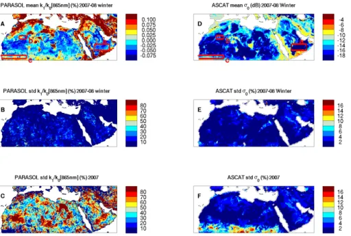
variability, especially during spring and summer months. This is partly related to the presence of aerosol in the atmospheric column at this time of the year (no aerosol cor-rection has been applied to the data). Marticorena et al. (2004) also observed this vari-ability increase in POLDER data and decided to use winter observations only for their analysis of the aerodynamic roughness length. Figure 1 (left panels) shows the mean

20

k1/k0coefficient for the 2007–2008 winter (November to February), along with the

vari-ability of this product over the winter and over the full 2007 year at 865 nm, for North Africa and the Arabian Peninsula. The variability is calculated as the standard deviation of thek1/k0over the meank1/k0, in percentage. Contrarily to POLDER (Laurent et al.,

2008), PARASOL provides quality data almost globally, during the winter months. The

25

k1/k0 coefficient should be independent from the wavelength (Roujean et al., 1992).

(7)

AMTD

5, 2933–2957, 2012

C. Prigent et al.

Title Page

Tables Figures

◭ ◮

Back Close

Full Screen / Esc

Discussion

P

a

per

|

Dis

cussion

P

a

per

|

Discussion

P

a

per

|

Discussio

n

P

a

per

|

correlation with the parameters at other wavelengths is consequently decreased (be-low 0.7). For three di_fferent zones (a sand desert area (a), a rocky desert region (b), and a semi-arid zone (c)) in the studied area, Fig. 2 (upper panels) shows the 2007 monthly mean time series of thek1/k0 parameters for PARASOL wavelengths.

Miss-ing data durMiss-ing summer months are related to aerosol contamination durMiss-ing the dust

5

season. The largest variability of the shorter wavelengths is clear. In the third region (right), some variability in the coefficient can also be observed even at the longer wave-lengths: this variability cannot be clearly related to vegetation phenology, as it is out of phase with the Normalized Difference Vegetation Index (NDVI) and the scatterometer responses to the vegetation (lower panels). For this study, the 865 nm observations

10

during the 2007 winter months will be used. Other parameters potentially related to the roughness have been examined, such as a bi-directionality index that represents the difference of the reflectances backward and forward over their sum, but these param-eters are very correlated with thek1/k0coefficient (∼0.9 for the longer wavelengths),

without any significant reduction in the noise level as compared tok1/k0.

15

2.2 ASCAT scatterometer satellite measurements

Active microwave observations over the entire globe have been available since 1991, from the ERS scatterometer at 5.25 GHz (1991 to 2001), from QuickScat at 13.4 GHz (1999–2009), and more recently from ASCAT at 5.25 GHz on board the European me-teorological satellite MetOp since 2006. In this study, ASCAT data are used. ASCAT

20

is the improved successor to the ERS scatterometer. Measurements at 5.25 GHz are very little affected by the atmosphere, and no contamination by the aerosols is ex-pected. Two sets of three antennas record the backscattering signals in different direc-tions, two of them points perpendicularly to the satellite track and the four others at 45◦_{, respectively two forward and two backward, to make observations in two 500 km}

25

wide swaths, on each side of the satellite ground track. The ASCAT provides measure-ments at 50 km spatial resolution, sampled every 25 km. First, the data are gridded on an equal area grid of 0.25◦

(8)

AMTD

5, 2933–2957, 2012

C. Prigent et al.

Title Page

Tables Figures

◭ ◮

Back Close

Full Screen / Esc

Discussion

P

a

per

|

Dis

cussion

P

a

per

|

Discussion

P

a

per

|

Discussio

n

P

a

per

|

between the ASCAT backscattering coefficientσ0 and the incident angle is calculated

for a month and the fitted value at 45◦ _{is kept, similar to the approach adopted for the} analysis of the ERS scatterometer in Prigent et al. (2005). Figure 1 (right panels) repre-sents the mean value of the backscattering coefficient at 45◦ _{for the winter 2007–2008} (November to February), for North Africa and the Arabian Peninsula, along with the

5

standard deviation of the information over the winter and over the full year. The scat-terometer data are very stable over time in the arid regions, with standard deviation of the order of the expected instrument noise (below 0.5 dB), in the arid regions. Over semi-arid regions, the scatterometer is sensitive to the presence of even sparse veg-etation, with an increase of the backscattering σ₀ with increasing vegetation density.

10

This is confirmed on Fig. 2, with very stable responses in the two desert regions (a and b), and a variability strongly correlated with the NDVI changes over the semi-arid area in the sub-Sahelian zone (c).

2.3 In situ data

Two types ofz0 in situ estimates are collected for comparisons with the satellite

ob-15

servations. These two sources of data have already been adopted in Marticorena et al. (2004, 2006) and in Prigent et al. (2005). The first source consists ofz₀estimates from wind profile obtained by Greeley et al. (1997) over Death Valley, Nevada, and Namibia. Since many measurements are performed locally for each site, thez0mean

value is computed for each one (G07 in Table 1). The second type ofz0 estimates is

20

derived from the geomorphologic methodology developed by Callot et al. (2000) for the Sahara and the Arabian Peninsula: it produces a map at 1◦

×1◦ spatial resolution. Homogeneous regions have already been selected from these geomorphologic esti-mates, for comparisons with satellite data (M04 and M06 in Table 1). In Marticorena et al. (2006), in situ z0 estimates from both methods (in situ and geomorphological)

25

(9)

AMTD

5, 2933–2957, 2012

C. Prigent et al.

Title Page

Tables Figures

◭ ◮

Back Close

Full Screen / Esc

Discussion

P

a

per

|

Dis

cussion

P

a

per

|

Discussion

P

a

per

|

Discussio

n

P

a

per

|

of 400 m width: we attempted to use this data set as well, but the spatial resolution of our satellite data and their high sensitivity to orography made the comparison with in situ measurements meaningless in such heterogeneous and mountain environments. It has been verified that the aeolian roughness lengths reported in Table 1 are also compatible with results obtained in wind tunnels over bare surfaces (Xue and Sun,

5

2002; Sherman and Farrell, 2008).

3 Relationship between satellite data and in situ roughness measurements

The comparison between the satellite and the in situ observations is limited to a pe-riod of time when both satellite data are available, with a quality compatible with our objective of estimating the roughness length. The winter 2007–2008 is selected: both

10

PARASOL and ASCAT data are available and PARASOL is little a_ffected by atmo-spheric aerosols during that season (see Sect. 2). The PARASOL observations are considered at their nominal 6 km spatial resolution, and the ASCAT data at ∼25 km spatial resolution.

3.1 PARASOL data versus aeolian roughness length

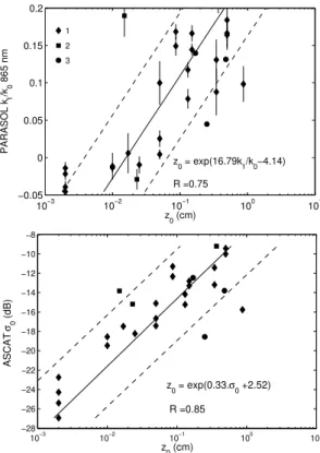
15

Previous studies (Marticorena et al., 1997, 2004, 2006; Laurent et al., 2005, 2006, 2008) evidenced the logarithmic relationship betweenz0andk1/k0over arid surfaces.

Figure 3 (upper panel) illustrates this log linear relationship betweenz0and PARASOL

k1/k0parameter at 865 nm. When thez0in situ estimates are not point measurements,

but are representative of an area, all PARASOL pixels within this area are averaged

20

(their mean and their std are indicated on Fig. 3). We verified that similar regressions are obtained with the other PARASOL channels that are highly correlated (see Sect. 2). 75 % of the variance is explained by this log linear relationship. Note that the regres-sion parameters estimated in this study are similar to those obtained by Marticorena et al. (2004) with POLDER, although the instruments and the time periods are different.

(10)

AMTD

5, 2933–2957, 2012

C. Prigent et al.

Title Page

Tables Figures

◭ ◮

Back Close

Full Screen / Esc

Discussion

P

a

per

|

Dis

cussion

P

a

per

|

Discussion

P

a

per

|

Discussio

n

P

a

per

|

3.2 ASCAT data versus aeolian roughness length

Greeley et al. (1997) showed the existence of a log linear relationship betweenz0and

the backscatteringσ0 at local scale and Prigent et al. (2005) confirmed it for the arid

and semi-arid regions, globally. The basis for this relation relies on a high sensitivity ofσ0 to the surface roughness when incidence angle values are above ∼35◦. Other

5

factors can interfere with the signal, such as volume scattering in sandy desert or vari-ations of the dielectric properties. The results from Prigent et al. (2005) with the ERS scatterometer were very encouraging and tended to show that the surface roughness dominates the signal in the arid and semi-arid regions. Figure 3 (lower panel) shows the log linear relationship between z0 and σ0 for the ASCAT observations at 25 km

10

spatial resolution, using the closest ASCAT 2007–2008 winter averaged observations to the in situ measurement. This regression explains 85 % of theσ0variance. Despite

the change in instrumentation (ERS to ASCAT), this relationship is very similar to the previously obtained one (Prigent et al., 2005), as expected.

3.3 Merging PARASOL and ASCAT data to estimate aeolian roughness length

15

Visible/near-infrared observations (PARASOL) can providez0estimates at high spatial

resolution, which is desirable for dust modeling at regional scale. However, these data are subject to contamination by clouds and aerosols, with quasi persistent missing data or low quality information in some regions. From scatterometer observations (ASCAT), robustz0 estimates can be derived, with no contamination from the atmosphere, but

20

with limited spatial resolution as compared to the visible/near-infrared estimates. Figure 4 compares the estimates from PARASOL and ASCAT, sorted by increasing values of the corresponding in situ data. A good correspondence is obtained between the two satellite products, despite their different spatial resolutions: the agreement be-tween the two satellite estimates is actually better than the agreement bebe-tween each

25

(11)

AMTD

5, 2933–2957, 2012

C. Prigent et al.

Title Page

Tables Figures

◭ ◮

Back Close

Full Screen / Esc

Discussion

P

a

per

|

Dis

cussion

P

a

per

|

Discussion

P

a

per

|

Discussio

n

P

a

per

|

i.e. higher than the correlations between the in situ z0 and each satellite information

separately (0.75 for PARASOL, and 0.85 for ASCAT). For pixels with a disagreement between the in situ data and one satellite, the two satellite values agree well. Note that the uncertainty on the in situ z0 estimate is not known and would be very difficult to

assess. The good consistency between the two satellite retrievals for these selected

5

sites suggests the possible merging of the two satellite information to benefit from their complementary strengths, at a global scale, namely the spatial resolution on one side and the robustness to atmospheric contamination on the other side.

A bi-linear regression is computed between the z0 in situ measurements on one

hand and the PARASOLk1/k0at 865 nm and the ASCAT backscattering on the other

10

hand. Figure 5 presents the retrieval versus the in situz0. The calculated regression,

representing 72 % of the variance, is as follows:

log(z0)=2.31+0.32×σ0+0.65×k1/k0. (2)

4 Aeolian roughness length estimate in arid and semi-arid regions at global scale

15

Maps ofz0 estimates are produced, from ASCAT and PARASOL separately, and from

their combination, using the previously established regressions (Fig. 6). Only regions withz₀lower than 0.1 cm are represented, corresponding to arid and semi-arid areas. For PARASOL, the averaged 2007–2008 winter observations are considered, as the other periods of the year can be contaminated by aerosols. Snow areas are filtered

20

out, using the National Snow and Ice Data Center (NSIDC, University of Colorado) (Armstrong and Brodzik, 2005). For ASCAT, z0 is estimated from the yearly average

(July 2007–June 2008): this makes it possible to have a better coverage of the ar-eas that are snow covered during the winter, as compared to the PARASOL selection. For the PARASOL-ASCAT combination, the ASCAT data is averaged over the full year

25

(12)

AMTD

5, 2933–2957, 2012

C. Prigent et al.

Title Page

Tables Figures

◭ ◮

Back Close

Full Screen / Esc

Discussion

P

a

per

|

Dis

cussion

P

a

per

|

Discussion

P

a

per

|

Discussio

n

P

a

per

|

data is projected onto the PARASOL grid, using distance-weighted means to the clos-est neighbors. When the PARASOL observations are not present (because of cloud contamination or snow for instance),z0is retrieved from ASCAT observations only.

Thez0derived from PARASOL (6 km) shows the expected structures over the very

arid regions (Fig. 6a), such as the Sahara or the Takla Makan. Similar results were

5

observed by Marticorena et al. (2004) and Laurent et al. (2005). Regions that are likely rather wet, such as India, West China, or West Africa below 10◦_{N also produce low}_z

0

(note that so far, thez0 visible/infrared estimates were not shown in the literature

out-side the very arid regions). This suggests that the visible/near-infrared observations are sensitive to other surface parameters and cannot provide an unambiguousz₀estimate

10

of arid and semi-arid regions globally, without additional filtering.

The z0 derived from ASCAT (Fig. 6b) is very close to the z0 derived from ERS by

Prigent et al. (2005) with 86 % correlation over the globe. A merged PARASOL-ASCAT

z0map is produced at 6 km spatial resolution (Fig. 6c). The major spatial structures of

the merged PARASOL-ASCAT map are very similar to the ASCAT only map. Note that

15

all erroneous structures present on the PARASOL-onlyz0estimates are suppressed.

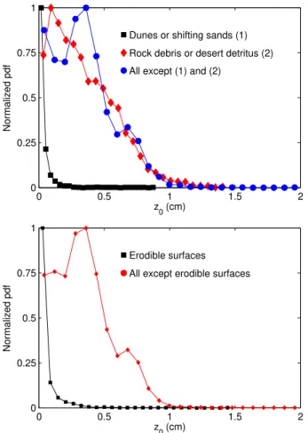
All “dunes and shifting sand” areas delineated by the FAO are clearly observed on this map, without any spurious patterns. As expected, all desert regions do not have low roughness length, and rocky deserts for instance such as the Tibetan plateau do not appear on the ASCAT derived map. Figure 7 (top) shows the histograms of thez0

20

derived from the PARASOL-ASCAT combination for “dunes and shifting sands” only (FAO classification), for “rock debris and desert detritus” (FAO classification) only, and for the remaining FAO classes. The sand dunes and shifting sands, as expected, show a very low aeolian roughness length, contrarily to rocky deserts (the two histograms are well separated). The mean value plus one standard deviation of the “dunes and shifting

25

sand” unit is equal to 0.11 cm, consistent with thez0variation range for bare surfaces

(13)

AMTD

5, 2933–2957, 2012

C. Prigent et al.

Title Page

Tables Figures

◭ ◮

Back Close

Full Screen / Esc

Discussion

P

a

per

|

Dis

cussion

P

a

per

|

Discussion

P

a

per

|

Discussio

n

P

a

per

|

Elevation Model at∼30−100 m scale from the Shuttle Radar Topography Mission. Fig-ure 6e presents this geomorphologocally-related index, where non-desert regions are masked (similar to Fig. 5a from Koven and Fung, 2008). The very large dust sources in the Bod ´el ´e region, in Malia/Mauritania, in Arabia, or in the Takla Makan appear on both the erodability maps and as very low aeolian roughness length from

PARASOL-5

ASCAT. In addition, regions of low roughness lengths such as the surroundings of Lake Eyre in Australia, the north of the Caspian Sea or South African deserts coincide with erodible areas, as defined by Koven and Fung (2008), although they did not appear on the FAO desert map. Figure 7 (bottom) presents the histograms ofz0 for the erodible

surfaces (as in Koven and Fung, 2008) as well as for all surfaces except the

erodi-10

ble ones. The erodible surfaces are clearly associated to very low roughness lengths, without ambiguities with other surface types.

5 Conclusions

In this study, we compare the potential of the visible/near-infrared observations and microwave backscattering measurements from satellite to estimate the aeolian

aero-15

dynamic roughness length over arid and semi arid regions, at global scale. We propose to merge the two sources of information to benefit from their complementary aspects, i.e. the high spatial resolution of the visible/near-infrared and the lack of sensitivity to atmospheric contamination of the active microwaves. A global map of the aeolian aerodynamic roughness length at 6 km resolution is derived from coincident satellite

20

observations and in situ roughness length measurements. The results are compared with success with existing information on arid regions. The aeolian roughness length dataset is available to the community, and will be soon tested in atmospheric dust transport models.

The implementation of dust emission models in regional or global models is very

25

(14)

AMTD

5, 2933–2957, 2012

C. Prigent et al.

Title Page

Tables Figures

◭ ◮

Back Close

Full Screen / Esc

Discussion

P

a

per

|

Dis

cussion

P

a

per

|

Discussion

P

a

per

|

Discussio

n

P

a

per

|

scales. For instance, in the ECMWF model, an aerodynamic roughness length is set to 1.3 m in deserts, at least two order of magnitude larger than the typical values of aeolian roughness length. Efforts are underway to relate these roughness length pa-rameters and possibly harmonize them (Darmenova et al., 2009). In a future study, remote sensing observations will be analyzed to estimate the aerodynamic roughness

5

length for land surface models, and possibly establish consistent scaling between the roughness lengths suitable for dust modeling as well as for momentum transfer in re-gional to global land surface modeling.

Acknowledgements. We are very grateful to F. M. Br ´eon for his help in the analysis of the PARASOL observations. We would also like to thank Beatrice Marticorena, Charlie Koven, 10

Bertrand Decharme, and Laurent Menut for valuable discussions and for sharing their datasets.

The publication of this article is financed by CNRS-INSU.

References

15

Alfaro, S. C. and Gomes, L.: Modeling mineral aerosol production by wind erosion: emission intensities and aerosol distributions in source areas, J. Geophys. Res, 106, 18075–18084, 2001.

Armstrong, R. L. and Brodzik, M. J.: Northern Hemisphere EASEGrid weekly snow cover and sea ice extent version 3, National Snow and Ice Data Center, Boulder, 2005.

20

(15)

AMTD

5, 2933–2957, 2012

C. Prigent et al.

Title Page

Tables Figures

◭ ◮

Back Close

Full Screen / Esc

Discussion

P

a

per

|

Dis

cussion

P

a

per

|

Discussion

P

a

per

|

Discussio

n

P

a

per

|

Darmenova, K., Sokolik, I. N., Shao, Y., Marticorena, B., and Bergametti, G.: Develop-ment of a physically based dust emission module within the Weather Research and Forecasting (WRF) model: assessment of dust emission parameterizations and input pa-rameters for source regions in Central and East Asia, J. Geophys. Res., 114, D14201, doi:10.1029/2008JD011236, 2009.

5

Food and Agricultural Organization (FAO): The digital Soil map of the world, 1 : 5 M scale, Land and Water Development Division, FAO, Rome, 2003.

Fung, A. K., Li, Z., and Chen, K. S.: Backscattering from a randomly rough dielectric surface, IEEE T. Geosci. Remote, 30, 356–369, 1992.

Gillette, D. and Passi, R.: Modeling dust emission caused by wind erosion, J. Geophys. Res., 10

93, 14233–14242, 1988.

Greeley, R., Blumberg, D. G., McHone, J. F., Dobrovolskis, A., Iversen, J. D., Lancaster, N., Rasmussen, K. R., Wall, S. D., and White, B. R.: Applications of space borne radar laboratory data to the study of aeolian processes, J. Geophys. Res., 102, 10971–10983, 1997.

Koven, C. D. and Fung, I.: Identifying global dust source areas using high resolution land surface 15

form, J. Geophys. Res., 113, D22204, doi:10.1029/2008JD010195, 2008.

Laurent, B., Marticorena, B., Bergametti, G., Chazette, P., Maignan, F., and Schmechtig, C.: Simulation of the mineral dust emission frequencies from desert areas of China and Mongolia using an aerodynamic roughness length map derived from the POLDER/ADEOS 1 surface products, J. Geophys. Res., 110, D18S04, doi:10.1029/2004JD005013, 2005.

20

Laurent B., Marticorena, B., Bergametti, G., and Mei, F.: Modeling mineral dust emissions from Chinese and Mongolian deserts, Global Planet. Change, 52, 121–141, 2006.

Laurent, B., Marticorena, B., Bergametti, G., Leon, J. F., and Mahowald, N. M.: Modeling mineral dust emissions from the Sahara desert using new surface properties and soil database, J. Geophys. Res., 113, D14218, doi:10.1029/2007JD009484, 2008.

25

Leroy, M., Deuz é, J. L., Br éon, F. M., Hautecoeur, O., Herman, M., Buriez, J. C., Tanre, D., Boufi és, S., Chazette, P., and Roujean, J. L.: Retrieval of aerosol properties and surface bi-directional reflectances from POLDER/ADEOS, J. Geophys. Res., 102, 17023–17037, 1997. MacKinnon, D. J., Clow, G. D., Tigges, R. K., Reynolds, R. L., and Chavez Jr., P. S.: Comparison

of aerodynamically and model-derived roughness lengths (z0) over diverse surfaces, Central 30

(16)

AMTD

5, 2933–2957, 2012

C. Prigent et al.

Title Page

Tables Figures

◭ ◮

Back Close

Full Screen / Esc

Discussion

P

a

per

|

Dis

cussion

P

a

per

|

Discussion

P

a

per

|

Discussio

n

P

a

per

|

Maignan, F., Br ´eon, F. M., and Lacaze, R.: Bidirectional reflectance of Earth targets: evaluation of analytical models using a large set of spaceborne measurements with emphasis on the hot spot, Remote Sens. Environ., 90, 210–220, 2004.

Marticorena, B. and Bergametti, G.: Modeling the atmospheric dust cycle: 1. Design of a soil-derived dust production scheme, J. Geophys. Res., 100, 16415–16430, 1995.

5

Marticorena, B., Bergametti, G., Aumont, B., Callot, Y., NaDoumi, C., and Legrand, M.: Modeling the atmospheric dust cycle: 2. Simulation of Saharan dust sources, J. Geophys. Res., 102, 4387–4404, 1997.

Marticorena, B., Chazette, P., Bergametti, G., Dulac, F., and Legrand, M.: Mapping the aerody-namic roughness length of desert surfaces from the POLDER/ADEOS bi-reflectance prod-10

uct, Int. J. Remote Sens., 25, 603–626, 2004.

Marticorena, B., Kardous, M., Bergametti, G., Callot, Y., Chazette, P., Khatteli, H., Le Hegarat-Mascle, S., Maille, M., Rajot, J.-L., Vidal-Madjar, D., and Zribi, M.: Surface and aerodynamic roughness in arid and semiarid areas and their relation to radar backscatter coefficient, J. Geophys. Res., 111, F03017, doi:10.1029/2006JF000462, 2006.

15

Prigent, C., Tegen, I., Aires, F., Marticorena, B., and Zribi, M.: Estimation of the aerodynamic roughness length in arid and semi-arid regions over the globe with the ERS scatterometer, J. Geophys. Res., 110, D09205, doi:10.1029/2004JD005370, 2005.

Raupach, M., Gillette, D., and Leys, J.: The effect of roughness elements on wind erosion threshold, J. Geophys. Res., 98, 3023–3029, 1993.

20

Roujean, J.-L., Leroy, M., and Deschamps, P.-Y.: A bidirectional reflectance model of the Earth’s surface for the correction of remote sensing data, J. Geophys. Res., 97, 20455–20468, 1992. Shao, Y.: A model for mineral dust emission, J. Geophys. Res., 106, 20239–20254, 2001. Sherman D. J. and Farrell, E. J.: Aerodynamic roughness lengths over movable

beds: comparison of wind tunnel and field data, J. Geophys. Res., 113, F02S08, 25

doi:10.1029/2007JF000784, 2008.

Tanr é, D., Br éon, F. M., Deuz é, J. L., Dubovik, O., Ducos, F., François, P., Goloub, P., Her-man, M., Lifermann, A., and Waquet, F.: Remote sensing of aerosols by using polarized, directional and spectral measurements within the A-Train: the PARASOL mission, Atmos. Meas. Tech., 4, 1383–1395, doi:10.5194/amt-4-1383-2011, 2011.

30

(17)

AMTD

5, 2933–2957, 2012

C. Prigent et al.

Title Page

Tables Figures

◭ ◮

Back Close

Full Screen / Esc

Discussion

P

a

per

|

Dis

cussion

P

a

per

|

Discussion

P

a

per

|

Discussio

n

P

a

per

|

Todd, M., Bou Karam, D., Cavazos, C., Bouet, C., Heinold, B., Baldasano, J., Cautenet, G., Koren, I., Perez, C., Solmon, F., Tegen, I., Tulet, P., Washington, R., and Zakey, A.: Quan-tifying uncertainty in estimates of mineral dust flux: an inter-comparison of model per-formance over the Bod ´el ´e Depression, Northern Chad, J. Geophys. Res, 113, D24107, doi:10.1029/2008JD010476, 2008.

5

Uno, I., Wang, Z., Chiba, M., Chun, Y. S., Gong, S. L., Hara, Y., Jung, E., Lee, S. S., Liu, M., Mikami, M., Music, S., Nickovic, S., Satake, S., Shao, Y., Song, Z., Sugimoto, N., Tanaka, T., and Westphal, D. L.: Dust model intercomparison (DMIP) study over Asia: overview, J. Geophys. Res., 111, D12213, doi:10.1029/2005JD006575, 2006.

Xian, X., Tao, W., Qingwei, S., and Weimin, Z.: Field and wind-tunnel studies of aerodynamic 10

roughness length, Bound.-Lay. Meteorol., 104, 151–163, 2002.

(18)

AMTD

5, 2933–2957, 2012

C. Prigent et al.

Title Page

Tables Figures

◭ ◮

Back Close

Full Screen / Esc

Discussion

P

a

per

|

Dis

cussion

P

a

per

|

Discussion

P

a

per

|

Discussio

n

P

a

per

|

Table 1.Aeolian aerodynamic roughness length in situ estimates from pedological observations (Marticorena et al., 2004, M04 in the table), and from wind profile estimates (Greeley et al., 1997, G07; Marticorena et al., 2006, M06).

Lat. max Lon. min Lat. min Lon. max z₀(cm) Ref.

20.73 –9.73 20.30 –9.30 0.002 M04

31.60 7.00 31.23 7.42 0.002 M04

21.80 –7.70 21.33 –7.25 0.002 M04

31.65 8.56 31.22 9.05 0.002 M04

23.70 0.98 23.30 1.36 0.010 M04

26.20 –7.48 25.80 –7.30 0.025 M04

21.70 5.33 21.25 5.80 0.050 M04

21.66 4.33 21.35 4.80 0.050 M04

30.70 11.15 30.25 11.20 0.150 M04

30.16 10.75 29.75 11.20 0.150 M04

25.70 8.16 25.30 8.53 0.500 M04

33.60 –1.30 33.20 –0.80 0.873 M04

26.42 –4.90 26.30 –4.45 0.050 M04

25.70 8.16 25.26 8.62 0.500 M04

26.20 8.28 25.76 8.53 0.500 M04

33.63 2.88 33.20 3.50 0.347 M04

33.62 3.52 33.20 4.02 0.347 M04

26.98 –3.73 26.76 –3.15 0.131 M04

27.78 –8.72 27.46 –8.28 0.131 M04

28.68 2.67 28.15 2.92 0.087 M04

29.77 2.97 29.23 3.58 0.087 M04

23.83 –8.37 23.45 –7.62 0.017 M04

22.50 0.62 22.28 0.88 0.010 M04

–23.40 14.73 –23.6 14.93 0.023 M04

36.43 –116.90 36.23 –116.70 0.369 G07

38.38 –116.25 38.13 –116.00 0.015 G07

33.26 10.47 33.26 10.47 0.480 M06

33.45 9.24 33.45 9.24 0.250 M06

(19)

AMTD

5, 2933–2957, 2012

C. Prigent et al.

Title Page

Tables Figures

◭ ◮

Back Close

Full Screen / Esc

Discussion

P

a

per

|

Dis

cussion

P

a

per

|

Discussion

P

a

per

|

Discussio

n

P

a

per

|

(20)

AMTD

5, 2933–2957, 2012

C. Prigent et al.

Title Page Abstract Introduction Conclusions References Tables Figures ◭ ◮ ◭ ◮ Back Close

Full Screen / Esc

Printer-friendly Version Interactive Discussion Discussion P a per | Dis cussion P a per | Discussion P a per | Discussio n P a per |

01 02 03 04 05 06 07 08 09 10 11 12 −0.4 −0.3 −0.2 −0.1 0 0.1 0.2 PARASOL k 1 /k0 (−) a

01 02 03 04 05 06 07 08 09 10 11 12 −0.4 −0.3 −0.2 −0.1 0 0.1 0.2 b

01 02 03 04 05 06 07 08 09 10 11 12 −0.4 −0.3 −0.2 −0.1 0 0.1 0.2

c 443 nm

565 nm 670 nm 765 nm 865 nm

01 02 03 04 05 06 07 08 09 10 11 12 0 0.05 0.1 0.15 0.2 0.25 0.3 NDVI (−) −25 −24 −23 −22 −21 −20

01 02 03 04 05 06 07 08 09 10 11 12 0 0.05 0.1 0.15 0.2 0.25 0.3 −20 −19 −18 −17 −16 −15

01 02 03 04 05 06 07 08 09 10 11 12 0 0.1 0.2 0.3 0.4 0.5

01 02 03 04 05 06 07 08 09 10 11 12−15 −14 −13 −12 −11 −10 ASCAT σ0 (dB) NDVI ASCAT σ₀

(21)

AMTD

5, 2933–2957, 2012

C. Prigent et al.

Title Page

Tables Figures

◭ ◮

Back Close

Full Screen / Esc

Discussion

P

a

per

|

Dis

cussion

P

a

per

|

Discussion

P

a

per

|

Discussio

n

P

a

per

|

10−3 10−2 10−1 100 101

−0.05 0 0.05 0.1 0.15 0.2

PARASOL k

1

/k0

865 nm

z₀ (cm) z

0 = exp(16.79k1/k0−4.14)

R =0.75

1

2

3

10−3 ₁₀−2 ₁₀−1 ₁₀0 ₁₀1

−28 −26 −24 −22 −20 −18 −16 −14 −12 −10 −8

ASCAT

σ0

(dB)

z₀ (cm)

z₀ = exp(0.33.σ₀ +2.52)

R =0.85

(22)

AMTD

5, 2933–2957, 2012

C. Prigent et al.

Title Page

Tables Figures

◭ ◮

Back Close

Full Screen / Esc

Discussion

P

a

per

|

Dis

cussion

P

a

per

|

Discussion

P

a

per

|

Discussio

n

P

a

per

|

1 1 1 1 1 1 2 1 2 1 1 1 1 1 1 1 1 1 1 3 3 1 1 2 3 1 1 1 1 0

0.2 0.4 0.6 0.8 1 1.2

Reference

z 0

(cm)

derived from PARASOL k₁/k₀ derived from ASCAT σ

0 (dB)

in situ

(23)

AMTD

5, 2933–2957, 2012

C. Prigent et al.

Title Page

Tables Figures

◭ ◮

Back Close

Full Screen / Esc

Discussion

P

a

per

|

Dis

cussion

P

a

per

|

Discussion

P

a

per

|

Discussio

n

P

a

per

|

10

−3

10

−2

10

−1

10

0

10

−3

10

−2

10

−1

10

0

modeled z

0

model

z

0

(cm)

z

0

= exp(0.65k

1

/k

0

+0.32

σ

+2.31)

R =0.85

1

2

3

(24)

AMTD

5, 2933–2957, 2012

C. Prigent et al.

Title Page

Tables Figures

◭ ◮

Back Close

Full Screen / Esc

Discussion

P

a

per

|

Dis

cussion

P

a

per

|

Discussion

P

a

per

|

Discussio

n

P

a

per

|

(25)

AMTD

5, 2933–2957, 2012

C. Prigent et al.

Title Page

Tables Figures

◭ ◮

Back Close

Full Screen / Esc

Discussion

P

a

per

|

Dis

cussion

P

a

per

|

Discussion

P

a

per

|

Discussio

n

P

a

per

|

0 0.5 1 1.5 2

0 0.25 0.5 0.75 1

z₀ (cm)

Normalized pdf

Dunes or shifting sands (1)

Rock debris or desert detritus (2)

All except (1) and (2)

0 0.5 1 1.5 2

0 0.25 0.5 0.75 1

z₀ (cm)

Normalized pdf

All except erodible surfaces Erodible surfaces