www.clim-past.net/12/2241/2016/ doi:10.5194/cp-12-2241-2016
© Author(s) 2016. CC Attribution 3.0 License.
Sea ice led to poleward-shifted winds at the Last Glacial
Maximum: the influence of state dependency
on CMIP5 and PMIP3 models
Louise C. Sime1, Dominic Hodgson1, Thomas J. Bracegirdle1, Claire Allen1, Bianca Perren1, Stephen Roberts1, and Agatha M. de Boer2
1British Antarctic Survey, Cambridge, UK
2Bert Bolin Centre for Climate Research, Department of Geological Sciences, Stockholm University, Stockhom, Sweden
Correspondence to:Louise C. Sime ([email protected])
Received: 30 March 2016 – Published in Clim. Past Discuss.: 15 April 2016
Revised: 6 September 2016 – Accepted: 13 October 2016 – Published: 19 December 2016
Abstract.Latitudinal shifts in the Southern Ocean westerly wind jet could drive changes in the glacial to interglacial ocean CO2inventory. However, whilst CMIP5 model results feature consistent future-warming jet shifts, there is consid-erable disagreement in deglacial-warming jet shifts. We find here that the dependence of pre-industrial (PI) to Last Glacial Maximum (LGM) jet shifts on PI jet position, or state de-pendency, explains less of the shifts in jet simulated by the models for the LGM compared with future-warming scenar-ios. State dependence is also weaker for intensity changes, compared to latitudinal shifts in the jet. Winter sea ice was considerably more extensive during the LGM. Changes in surface heat fluxes, due to this sea ice change, probably had a large impact on the jet. Models that both simulate realis-tically large expansions in sea ice and feature PI jets which are south of 50◦S show an increase in wind speed around 55◦S and can show a poleward shift in the jet between the PI and the LGM. However, models with the PI jet positioned equatorwards of around 47◦S do not show this response: the sea ice edge is too far from the jet for it to respond. In mod-els with accurately positioned PI jets, a +1◦ difference in
the latitude of the sea ice edge tends to be associated with a
−0.85◦shift in the 850 hPa jet. However, it seems that around
5◦ of expansion of LGM sea ice is necessary to hold the jet in its PI position. Since the Gersonde et al. (2005) data support an expansion of more than 5◦, this result suggests
that a slight poleward shift and intensification was the most likely jet change between the PI and the LGM. Without the effect of sea ice, models simulate poleward-shifted wester-lies in warming climates and equatorward-shifted westerwester-lies
in colder climates. However, the feedback of sea ice counters and reverses the equatorward trend in cooler climates so that the LGM winds were more likely to have also been shifted slightly poleward.
1 Introduction
The concentration of CO2 in the atmosphere decreases by
∼90 parts per million between warm interglacial and cold
glacial climate states due to oceanic storage of the excess car-bon (Sigman et al., 2010). Mechanisms behind this enhanced ocean storage are still unresolved. One hypothesis invokes latitudinal shifts in the Southern Ocean westerly wind belt. An equatorward, or weaker, westerly wind jet could suppress deep water ventilation, leading to carbon becoming trapped in cold dense waters (Toggweiler et al., 2006; Sigman et al., 2010; Denton et al., 2010).
ef-fects on atmospheric carbon, with a rise of only 3 to 9 ppm CO2under both a northward and a southward 10◦shift of the surface jet. These results are similar to those obtained using some simpler ocean models (Menviel et al., 2008; Tschumi et al., 2008; d’Orgeville et al., 2010). However, the effects on ocean circulation and biology are complex and non-linear, with competing effects from physical and biological carbon pumps. Thus it is difficult to know if these model-based stud-ies are sufficiently accurate to constrain the CO2impact of a specified wind shift. So whilst most, though not all (e.g. Lee et al., 2011), ocean and carbon modelling results do not sup-port the idea that shifts in the westerly wind belt played a dominant role in coupling atmospheric CO2rise and global temperature, there is, as yet, no definitive answer to this ques-tion.
Jet shifts have been proposed to modify other aspects of the climate–CO2 system. Iron-rich dust borne by Southern Hemisphere winds is thought to increase Southern Ocean productivity (Kohfeld et al., 2005). Lamy et al. (2014) show that large-scale southern hemispheric climate forcings, likely wind related, enhanced cold glacial period dust mobilisa-tion in Australia, New Zealand, and Patagonia. Ferrari et al. (2014) hypothesise a Southern Ocean dividing latitude be-tween negative and positive buoyancy forcing at the edge of the summer sea ice edge, with knock-on impacts for ocean dynamics. Völker and Köhler (2013) show that when the at-mospheric jet shifts poleward, summer sea ice extends, likely due to enhanced heat loss to the atmosphere. Thus both dust and buoyancy forcing may provide an additional means for jet changes to influence glacial to interglacial climate shifts.
A wide range of palaeodata has been interpreted as evi-dence for glacial to interglacial jet shifts. These data include proxies, or direct measurements of, terrestrial moisture, dust deposition, sea surface temperatures, and ocean productiv-ity. Kohfeld et al. (2013) find that purely based on these palaeodata, one can hypothesise a variety of wind change scenarios including: no change, a southward shift, and a northward shift. It remains an extraordinarily difficult task to constrain glacial to interglacial jet shifts and intensifica-tions based on data alone (Hodgson and Sime, 2010). Whilst Sime et al. (2013) find that the moisture change palaeodata can be accurately modelled under a no jet shift scenario, Ko-hfeld et al. (2013) suggest that an equatorward jet shift, or intensification, could also be consistent with the majority of the palaeodata. Efforts to help solve this jet change problem using GCMs have benefitted from the fifth Coupled Model Intercomparison Project (CMIP5), specifically the third Pa-leoclimate Modelling Intercomparison Project (PMIP3), and its predecessor PMIP2 (Braconnot et al., 2007, 2012; Taylor et al., 2011). PMIP2 and PMIP3 have provided ensembles of LGM and pre-industrial (PI) climate simulations, where each model is run under the same boundary conditions, permit-ting inter-model comparisons and insight into crucial wind change mechanisms (e.g. Roche et al., 2012; Rojas, 2013; Chavaillaz et al., 2013; Sime et al., 2013; Liu et al., 2015).
Existing analyses of PMIP2 and PMIP3 LGM simulation ensembles show considerable inter-model disagreement in PI to LGM southern hemispheric jet changes (Rojas, 2013; Chavaillaz et al., 2013). This is despite the fact that nearly all CMIP5 models exhibit a poleward shift, and all models a strengthening, of the surface jet from 1900 to 2100 (Brace-girdle et al., 2013). Indeed Chavaillaz et al. (2013) find that future-warming scenario RCP4.5 (Representative Concentra-tion Pathway 4.5) shifts in the 850 hPa jet can be largely explained by tropospheric temperature differences between the southern high latitudes and the tropics. Bracegirdle et al. (2013) and Kidston and Gerber (2010) examine another as-pect: state dependency for Southern Ocean jet shifts and in-tensity changes, where state dependency is defined as the de-pendence of jet shifts on the start jet position. Bracegirdle et al. (2013) find that for some oceanic sectors, particularly the Pacific, the starting position of the jet (state dependence) explains more than 85 % of the jet shift variance found be-tween the different CMIP5 future-warming scenario simula-tions. This implies that the start latitude of the jet is poten-tially a strong contender as an explanation for CMIP5-PMIP3 inter-model jet shift differences. Additionally, whilst tropi-cal temperature changes dominate the future-warming wind changes, high-latitude temperature changes are as significant to the winds during the deglacial-warming (Chavaillaz et al., 2013). Sea ice is thus also highlighted as being particularly significant for the accurate jet simulations (Chavaillaz et al., 2013; Sime et al., 2013). Here we investigate past-cooling LGM state dependency, sea ice, and changes in the Southern Ocean westerly wind jet using CMIP5-PMIP3 output.
2 Data: CMIP5-PMIP3 simulations
CMIP5-PMIP3 PI and LGM simulations are run with full dy-namic ocean and sea ice models. The LGM simulations all follow the PMIP3 protocol (https://wiki.lsce.ipsl.fr/pmip3/ doku.php/pmip3:design:21k:final): orbital parameters are set to their 21 000 years ago values and concentrations of at-mospheric greenhouse gases are set to 185 ppm for CO2, 350 ppb for CH4, and 200 ppb for N2O. All models use the PMIP3 LGM ice sheet or ICE5.2G ice sheet configurations (Chavaillaz et al., 2013). Simulations are run for long enough to allow the atmosphere and ocean to reach quasi-equilibrium (Braconnot et al., 2012; Rojas, 2013).
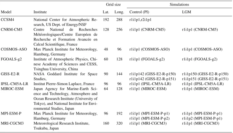
Table 1.List of all CMIP5-PMIP3 simulations used in this study. The individual simulations (r< N >i< M >p<L>) formatted as shown below (e.g. “r3i1p21” with r for “realisation”, i for “initialization method indicator”, and p for “perturbed physics”) distinguishes among closely related simulations by a single model.
Grid size Simulations
Model Institute Lat. Long. Control (PI) LGM
CCSM4 National Center for Atmospheric
Re-search, US Dept. of Energy/NSF
192 288 r1i1p1,r2i1p1
CNRM-CM5 Centre National de Recherches
Météorologiques/Centre Européen de Recherche et Formation Avancée en Calcul Scientifique, France
128 256 r1i1p1 (CNRM-CM5) r1i1p1 (CNRM-CM5)
COSMOS-ASO Max Planck Institute for Meteorology,
Hamburg, Germany
48 96 r1i1p1 (COSMOS-ASO) r1i1p1 (COSMOS-ASO)
FGOALS-g2 Institute of Atmospheric Physics,
Chi-nese Academy of Sciences and CESS, Tsinghua University, China
60 128 r1i1p1 (FGOALS-g2) r1i1p1 (FGOALS-g2)
GISS-E2-R NASA Goddard Institute for Space
Studies,
90 144 r1i1p142 (GISS-E2-R-p150)
r1i1p142 (GISS-E2-R-p151)
r1i1p150 (GISS-E2-R-p150) r1i1p151 (GISS-E2-R-p151)
IPSL-CM5A-LR Institut Pierre-Simon Laplace, France 96 96 r1i1p1 (IPSL-CM5A-LR) r1i1p1 (IPSL-CM5A-LR)
MIROC-ESM Japan Agency for Marine-Earth
Sci-ence and Technology, Atmosphere and Ocean Research Institute (University of Tokyo), and National Institute for Envi-ronmental Studies, Japan
64 128 r1i1p1 (MIROC-ESM) r1i1p1 (MIROC-ESM)
MPI-ESM-P Max Planck Institute for Meteorology,
Hamburg, Germany
96 192 r1i1p1 (MPI-ESM-P-p1)
r1i1p1 (MPI-ESM-P-p2)
r1i1p1 (MPI-ESM-P-p1) r1i1p2 (MPI-ESM-P-p1)
MRI-CGCM3 Meteorological Research Institute,
Tsukuba, Japan
160 320 r1i1p1 (MRI-CGCM3) r1i1p1 (MRI-CGCM3)
2.1 Southern Ocean wind jet diagnostics
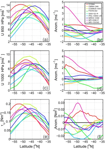
The choice of Southern Ocean jet diagnostic can influence apparent glacial to interglacial wind change results (Liu et al., 2015). Previous authors have used surface winds (Kim et al., 2003), above-surface winds, or surface shear stress (Otto-Bliesner et al., 2006). Where sea ice replaces open water, each of these diagnostics shows a different response (Sime et al., 2013; Liu et al., 2015). Sea ice affects sur-face roughness and near-sursur-face stratification of the bound-ary layer, this can lead to quite different results for glacial to interglacial changes in different wind diagnostics and shear stress (Fig. 1). For this reason, we concentrate on the above surface (850 hPa) winds, given that any model specific spec-ification of sea ice effects tends to have a lesser impact on this diagnostic (Sime et al., 2013). However, given the im-portance of surface wind speed and shear stress for driving the Southern Ocean and global ocean circulation and hence CO2 exchange, some discussion of all of these three wind diagnostics is included in this study.
When calculating jet intensity and position for each di-agnostic, we use a cubic spline interpolation to quantify the jet maximum and determine its latitude. Jet shifts are de-fined here as PI to LGM changes in the latitudinal position of the zonal mean maximum in the jet. Data are regridded to a consistent 0.1◦resolution before these calculations are
per-formed. In addition to these zonal mean diagnostics, we also assess individual ocean sectors results. In these cases, sectors are defined by longitude ranges as follows: Atlantic sector (290 to 20◦), Indian sector (20 to 150◦), and Pacific sector
(150 to 290◦). Jet diagnostics are calculated for the annual mean in the Southern Hemisphere 850 hPa wind component; the annual mean 1000 hPa westerly wind is used as an indi-cator for surface wind. This diagnostic is used in lieu of the 10 m surface westerly wind speed “uas” field, because “uas” is not available for LGM simulations for two CMIP5 models. We also calculate the zonal shear stressτU, “jet” position and
intensity. Required variables (“ua” and “tauu”) were down-loaded from the CMIP5 data archive between September and October in 2014.
All CMIP5 models show an equatorward bias in the present-day zonal mean surface jet position. The ensemble of present-day CMIP5 simulations show a mean equatorward bias of 3.3◦(inter-model standard deviation of±1.9◦) in the
repre-−55 −50 −45 −40 −35 2 4 6 8 10 12 14 U 850 HPa [ms −1 ]
−55 −50 −45 −40 −35 −2 −1 0 1 2 3 4 5 Anom. [ms −1 ]
−55 −50 −45 −40 −35 0 2 4 6 8 10 U 1000 HPa [ms −1 ]
−55 −50 −45 −40 −35 −2 −1 0 1 2 3 4 5 Anom. [ms −1 ]
−55 −50 −45 −40 −35 0
0.05 0.1 0.15 0.2
Latitude [oN]
τ U
[Nm
2 ]
−55 −50 −45 −40 −35 −0.02 −0.01 0 0.01 0.02 0.03
Latitude [oN]
Anom. [Nm 2 ] (a) (b) (c) (d) (e) (f) CCSM4 CNRM−CM5 COSMOS−ASO FGOALSg2 GISS−E2−R IPSL−CM5A−LR MIROC−ESM MPI−ESM−P MRI−CGCM3
Figure 1.Zonal mean Southern Ocean winds.(a)PI wind speed
U at 850 hPa, (b) LGM− PI anomaly, (c)PI wind speed U at 1000 hPa, and the ERA-Interim Bracegirdle et al. (2013) latitudi-nal position of the surface jet maximum to represent the observa-tional position (d) and the 1000 hPa LGM−PI anomaly, (e)PI surface shear stressτU, and(f)theτULGM−PI anomaly. Colours as shown in the legend in panel(b)denote the individual models. All values are annual means.
sentation may not be critical. The equatorward jet biases are mainly associated with the Indian and Pacific sectors.
2.2 The sea ice edge
Where available, sea ice concentration data were downloaded for the model simulations. The sea ice edge was calculated using a mean annual sea ice concentration of 15 %. For a few model simulations sea ice concentration data were not avail-able. In this case a best fit relationship between sea surface temperature and sea ice edge, derived from the models where both output were available, was used to estimate the sea ice edge (COSMOS-ASO and IPSL-CM5A-LR).
3 Results
3.1 Jet changes and state dependency
We focus in this study on the PI and LGM CMIP5-PMIP3 simulations. Table 2 indicates a wide range of PI to LGM lat-itudinal jet shifts across the PMIP3 simulations, varying from
+2.0 to−4.5◦for the 850 hPa jet. The mean 850 hPa jet shift
for the nine models is small: −0.2◦ (inter-model standard
deviation of±2.1◦). The mean surface jet shift for the nine
models is−0.9◦(inter-model standard deviation of±1.6◦).
The median shift for both 850 and 1000 hPa is 0◦. Similar inter-model variation appears in the jet intensity changes (Ta-ble 2).
Following the Bracegirdle et al. (2013) approach, we cal-culate state dependency for Southern Ocean jet shifts and in-tensity changes across the various oceanic sectors, i.e. the dependence of PI to LGM jet shifts with PI jet position. Feedbacks within the troposphere have been used to explain state dependence in previous studies (e.g. Kidston and Ger-ber, 2010). We find that state dependency can explain up to 56 % of the variance in PI to LGM jet shifts in the At-lantic (r= −0.75, N=9, for τU) and 41 % in the Indian
Ocean (r= −0.64,N=9, forτU). State dependency is much
weaker in the Pacific; here any influence is negligible. 850 and 1000 hPa results are always very similar (not shown). We find state dependence is stronger for theτU jet than the
850 hPa jet (Fig. 2) due largely to the MRI-CGCM3 850 hPa outlier. With the anomalous MRI-CGCM3 850 hPa wind re-sult removed from the calculation, we obtain similar rere-sults between 850 hPa and τU. For the whole of the Southern
Ocean, the variance explained by state dependency is 38 % (r= −0.62,N=9, forτU).
Whilst these CMIP5-PMIP3 results bear similarities to the Bracegirdle et al. (2013) CMIP5-RCP8.5 analysis of state dependence, they also show distinct differences. Over the Atlantic sector Bracegirdle et al. (2013) find that the corre-lation, calculated between present-day and RCP8.5 CMIP5 output, is relatively weak (r= −0.39) compared with the
correlations over the Indian sector (r= −0.50) and Pacific
sector (r= −0.91). Interestingly, Bracegirdle et al. (2013)
also find that correlation results over the Atlantic are con-ditional on omitting model MRI-CGCM3, which is again an influential outlier due to jumps in jet position.
For jet intensity Bracegirdle et al. (2013) find the state de-pendence is generally weaker than for position; we find a similar result here. The state dependency in intensity change can explain only 25 % (r= −0.50,N=9, forτU) of the PI
to LGM change.
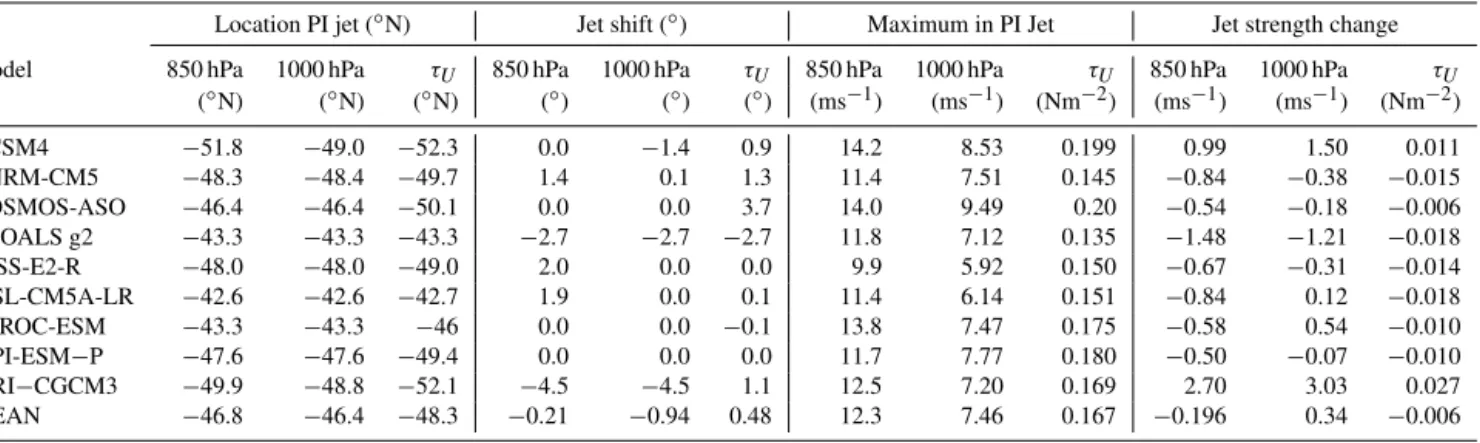
Table 2.The Southern Ocean westerly winds jet position, jet strength, and PI to LGM changes in jet position and strength.
Location PI jet (◦N) Jet shift (◦) Maximum in PI Jet Jet strength change Model 850 hPa 1000 hPa τU 850 hPa 1000 hPa τU 850 hPa 1000 hPa τU 850 hPa 1000 hPa τU
(◦N) (◦N) (◦N) (◦) (◦) (◦) (ms−1) (ms−1) (Nm−2) (ms−1) (ms−1) (Nm−2)
CCSM4 −51.8 −49.0 −52.3 0.0 −1.4 0.9 14.2 8.53 0.199 0.99 1.50 0.011
CNRM-CM5 −48.3 −48.4 −49.7 1.4 0.1 1.3 11.4 7.51 0.145 −0.84 −0.38 −0.015 COSMOS-ASO −46.4 −46.4 −50.1 0.0 0.0 3.7 14.0 9.49 0.20 −0.54 −0.18 −0.006 FGOALS g2 −43.3 −43.3 −43.3 −2.7 −2.7 −2.7 11.8 7.12 0.135 −1.48 −1.21 −0.018 GISS-E2-R −48.0 −48.0 −49.0 2.0 0.0 0.0 9.9 5.92 0.150 −0.67 −0.31 −0.014 IPSL-CM5A-LR −42.6 −42.6 −42.7 1.9 0.0 0.1 11.4 6.14 0.151 −0.84 0.12 −0.018
MIROC-ESM −43.3 −43.3 −46 0.0 0.0 −0.1 13.8 7.47 0.175 −0.58 0.54 −0.010
MPI-ESM−P −47.6 −47.6 −49.4 0.0 0.0 0.0 11.7 7.77 0.180 −0.50 −0.07 −0.010 MRI−CGCM3 −49.9 −48.8 −52.1 −4.5 −4.5 1.1 12.5 7.20 0.169 2.70 3.03 0.027 MEAN −46.8 −46.4 −48.3 −0.21 −0.94 0.48 12.3 7.46 0.167 −0.196 0.34 −0.006
−60 −55 −50 −45 −40
−10 −5 0 5 10
Jet position (degrees)
Jet shift (degrees)
Zonal mean
r = 0.15 (−0.21) r = −0.62
−60 −55 −50 −45 −40
−10 −5 0 5 10
Jet position (degrees)
Jet shift (degrees)
Atlantic
r = −0.14 (−0.49) r = −0.75
−60 −55 −50 −45 −40
−10 −5 0 5 10
Jet position (degrees)
Jet shift (degrees)
Indian
r = −0.54 (−0.78) r = −0.64
−60 −55 −50 −45 −40
−10 −5 0 5 10
Jet position (degrees)
Jet shift (degrees)
Pacific
r = −0.01 (−0.14) r = −0.099
(a) (b)
(c) (d)
CCSM4 CNRM−CM5 COSMOS−ASO FGOALSg2 GISS−E2−R IPSL−CM5A−LR MIROC−ESM MPI−ESM−P MRI−CGCM3 MODELS:
Wind speed (850 hPa) Surface τU
VARIABLES
Figure 2.The state dependence of jet latitudinal shifts.(a)Scatter plot of PI annual mean Southern Ocean jet position versus LGM minus PI change in the CMIP5-PMIP3 models. (b), (c), and(d) show the same but for individual ocean sectors: Atlantic, Indian, and Pacific, as marked. The Atlantic sector is defined as 290 to 20◦, the Indian as 20 to 150◦, and the Pacific as 150 to 290◦. In-dividual symbols indicate inIn-dividual models, as marked in the leg-end in panel (a). The jet is defined using the zonal 850 hPa wind speed (red) and surface shear stress (blue). Dashed lines indicate the model mean position and model mean shift for each panel. Speci-fiedrvalues indicate the correlation coefficient; bracketed 850 hPa r values are calculated excluding the MRI-CGCM3 model.
Corre-lation coefficients and reCorre-lationships using 1000 hPa “surface wind speeds” are almost identical to those using 850 hPa.
now look at the factors which are most likely to drive these changes.
3.2 The impact of sea ice
The most recent compilation of LGM sea surface temper-ature data is the MARGO dataset (MARGO Project Mem-bers, 2009). Although the coverage of MARGO data is good in tropical regions, it is sparse poleward of 40◦S (MARGO
Project Members, 2009). However, Gersonde et al. (2005) provide LGM sea surface temperature and sea ice data from 122 Southern Ocean sediment core sites. These data suggest that LGM sea ice extended in the Atlantic and Indian sec-tor to close to 47◦S and in the Pacific sector to 57◦S – a PI to LGM equatorward expansion of between 7 and 10◦in latitude. This is a large change, particularly compared with the sea ice changes which occur during most future-warming scenario CMIP5 simulations.
All CMIP5-PMIP3 models for which we can retrieve sea ice output show an LGM expansion of sea ice in the South-ern Hemisphere (Table 3). There is considerable variabil-ity between the models. Expansions range between 2.1 and 7.0◦(Fig. 4, Table 3). Only two models, CCSM4 and
MRI-CGCM3 (with Gersonde et al. (2005) data agreements of 87 and 88 %; see Appendix A), appear to yield an accurate simu-lation of LGM sea ice extent (Table 3) and some of the largest equatorward expansions of sea ice at 5.6 and 7.0◦, respec-tively.
Changes in sea ice extent are associated with relatively strong surface heat flux anomalies, which can be as large as 100 W m−2(Alexander et al., 2004). A strong non-linearity of wind response can thus be generated, dependent on the location of the resultant changes in meridional temperature gradients in the atmosphere. For example, surface cooling due to an expansion of sea ice causes an anomalous increase in the meridional temperature gradient adjacent to the newly ice-covered ocean. If this increased gradient lies immedi-ately poleward of the jet and its associated baroclinic zone, it can be more effective at influencing developing baroclinic waves and the latitude of the jet. Support for this idea is also found in the results of Chen et al. (2010) and Brayshaw et al. (2008), where changes in surface heat fluxes have the largest impact when they are approximately co-located with the maximum in the meridional temperature gradient.
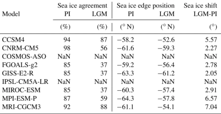
tem-Table 3. The model–data agreement from the sea ice edge latitude, the mean zonal sea ice edge latitude, and the PI to LGM jet shift. Simulation results are bi-linearly interpolated to each Gersonde et al. (2005) observation site. Model–data agreement is then calculated by classing simulated sea ice as present or absent, analogous to the exact metric defined by Sime et al. (2013). A simple agreement percentage metric is then calculated using the equivalent Gersonde et al. (2005) sea ice (present or absent) observations.
Sea ice agreement Sea ice edge position Sea ice shift
Model PI LGM PI LGM LGM-PI
(%) (%) (◦N) (◦N) (◦)
CCSM4 94 87 −58.2 −52.6 5.57
CNRM-CM5 98 56 −61.6 −59.3 2.27
COSMOS-ASO NaN NaN NaN NaN NaN
FGOALS-g2 85 37 −59.2 −56.4 2.78
GISS-E2-R 85 37 −63.3 −61.2 2.05
IPSL-CM5A-LR NaN NaN NaN NaN NaN
MIROC-ESM 85 37 −60.3 −57.4 2.91
MPI-ESM-P 87 59 −64.3 −57.8 6.57
MRI-CGCM3 92 88 −61.1 −54.1 7.04
Jet strength (normalised)
−3 −2 −1 0 1 2 3
−3 −2 −1 0 1 2 3
Jet strength change (normalised)
Zonal mean
r = 0.34 (0.56) r = 0.50 (0.82)
Jet strength (normalised)
−3 −2 −1 0 1 2 3
−3 −2 −1 0 1 2 3
Jet strength change (normalised)
Atlantic
r = 0.25 (0.64) r = −0.01 (0.59)
−3 −2 −1 0 1 2 3
−3 −2 −1 0 1 2 3
Jet strength (normalised)
Jet strength change (normalised)
Indian
r = −0.31 (−0.45) r = 0.43 (0.56)
−3 −2 −1 0 1 2 3
−3 −2 −1 0 1 2 3
Jet strength (normalised)
Jet strength change (normalised)
Pacific
r = 0.35 (0.50) r = 0.27 (0.41)
(a) (b)
(c) (d)
CCSM4 CNRM−CM5 COSMOS−ASO FGOALSg2 GISS−E2−R IPSL−CM5A−LR MIROC−ESM MPI−ESM−P MRI−CGCM3 MODELS:
Wind speed (850 hPa) Surface τU
VARIABLES
Figure 3. The state dependence of jet intensity (wind speed) changes. (a)Scatter plot of PI annual mean Southern Ocean jet strength versus LGM minus PI change in the CMIP5-PMIP3 mod-els. Zonal mean(a), Atlantic sector(b), Indian sector(c), and Pa-cific sector(d). Results are normalised by subtracting the mean of all models, and dividing through by the standard deviation of all models. Caption and results as Fig. 2.
perature gradient over the troposphere give larger westerly wind increases over the troposphere, this is actually because increases in horizontal temperature gradient lead to increases in westerly wind with height. These wind changes are gen-erally quite small near the surface and either increase or de-crease with height, depending on the sign of the temperature gradient change.
When looking at all models, there are some commonali-ties in the meridional structure in wind and temperature gra-dient changes. Between the top and 200 hPa level, poleward of 50◦S the temperature gradient increases resulting in an in-crease in westerly wind speed,U. Equatorward of 50◦S the
temperature gradient tends to decrease, with the strongest de-crease between 50 and 300 hPa. Upper and mid-tropospheric
Ualso decreases in all models equatorward of around 50◦S.
Below 400 hPa there tends to be an increase in the meridional temperature gradient poleward of around 40◦S, but there is considerable inter-model variability in the details of the tem-perature gradient changes and in associated wind changes.
As the above implies, we find that the key differences in westerly winds and meridional temperature gradients changes are a function of state dependence and sea ice. In-deed, based on state dependence (PI jet position) and sea ice changes, models can be roughly classed into four groups. CCSM4 and MRI-CGCM3, in the first group (Figs. 5a, b and 6a, b), both simulate large expansions in sea ice (of 5.6 and 7◦, respectively) and feature the most southerly posi-tioned jets (at 51◦S±1.1◦). This jet position tends to leave
U sensitive to expansions in sea ice. The large increases in
the meridional temperature gradient, especially around 55◦S from 1000 to about 650 hPa, thus tally with the increases inU around these latitudes and also result in a PI to LGM
poleward shift in the jet in both models, especially in MRI-CGCM3.
In the second group, whilst GISS-ER-R and CNRM-CM5 (Figs. 5c, d and 6c, d) have PI jets which are positioned rel-atively far to the south (at 48◦S±0.3◦), both feature rather
small LGM expansions in sea ice (of around 2◦). The
resul-tant small polar atmospheric cooling causes little change in the meridional temperature gradient.Utends to weaken over
the Southern Ocean latitudes, likely due to the overall atmo-spheric cooling. These two models show a slight equatorward shift in their jets between the PI and the LGM.
In the third group, COSMOS-ASO and MPI-ESM-P (Figs. 5e, f and 6e, f) have PI jets positioned at 47◦S±0.6◦
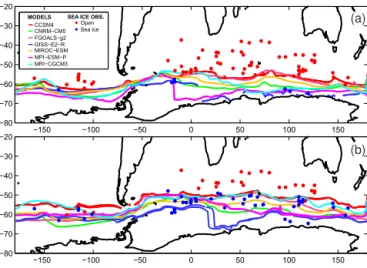
mod-−150 −100 −50 0 50 100 150 −80 −70 −60 −50 −40 −30 −20
−150 −100 −50 0 50 100 150
−80 −70 −60 −50 −40 −30 −20 CCSM4 CNRM−CM5 FGOALS−g2 GISS−E2−R MIROC−ESM MPI−ESM−P MRI−CGCM3 Open Sea ice
MODELS SEA ICE OBS. (a)
(b)
Figure 4.Sea ice from models and the Gersonde et al. (2005) ob-servations for(a)the PI and(b)the LGM. Coloured dots show open water (red) and inferred sea ice (blue). The differing coloured lines show the annual mean 15% sea ice extent for individual models. See legend for colours.
els less sensitive to the LGM expansion of sea ice: they show a slight weakening of U and no jet shifts. It seems that the
storm track and its associated baroclinic zone are not signif-icantly affected by these sea ice increases, or by associated meridional temperature gradient changes, because they hap-pen far poleward of the baroclinic jet zone.
In the last group, FGOALS-G2, IPSL-CM5A-LR, and MIROC-ESM (Figs. 5g, h, i and 6g, h, i) all have very northerly positioned PI jets (at 43◦S±0.5◦), due they also
all show a rather small (less than 3◦) LGM increase in sea
ice extent. The jets in these models thus seem to be respond-ing to influences other than sea ice: possibly tropical changes or sea surface temperature changes nearer 43◦have more im-pact. Chavaillaz et al. (2013) find a quasi-linear relationship between the jet shifts and tropical temperature changes in the atmosphere, where polar temperatures are held constant, sug-gesting that tropical changes may be a stronger influence on these models.
3.2.1 The relationship between sea ice extent and jet position
In simulations with more poleward (i.e. accurately) posi-tioned PI jets, the examination above of jet and sea ice changes suggests that PI to LGM wind changes are strongly related to sea ice extent. Figure 7a shows that the PI jet po-sition is inversely related to sea ice extent in models with the most accurately positioned PI jets. We find that an equator-wards sea ice edge correlates with a poleward jet position (r= −0.95 for the PI, andr= −0.91 for the LGM). Whilst
correlations are strongest for 850 hPa winds, similar results are obtained using 1000 hPa andτU (r <−0.80).
−80 −60 −40 −20 200 400 600 800 COSMOS−ASO hPa
−80 −60 −40 −20 200 400 600 800 MPI−ESM−P hPa
−80 −60 −40 −20 200 400 600 800 FGOALS G2 hPa
−80 −60 −40 −20 200 400 600 800 IPSL−CM5A−LR hPa
−80 −60 −40 −20 200 400 600 800 MIROC−ESM Latitude hPa
−5 0 5
−80 −60 −40 −20 200 400 600 800 CCSM4 hPa
−80 −60 −40 −20 200 400 600 800 MRI−CGCM3 hPa
−80 −60 −40 −20 200 400 600 800 GISS−E2−R hPa
−80 −60 −40 −20 200 400 600 800 CNRM−CM5 hPa (a) (b) (c) (d) (e) (f) (g) (h) (I)
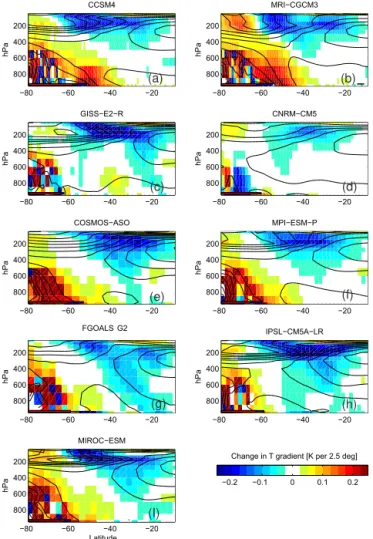
Figure 5.Change is the zonal mean wind velocity component in the westerly directionU (LGM−PI) throughout the atmosphere (shaded). Black contours show meanU for the PI. Red and blue bars at the bottom left of each panel indicate the extent of the zonal mean sea ice for the PI and LGM, respectively. Individual panels are labelled to indicate individual models. All values are annual means.
In terms of PI to LGM jet shifts, if we apply a linear least-squares fit, we find that a 1◦difference in the sea ice edge suggests a−0.85◦shift in the 850 hPa jet (r= −0.80;
N=5). These results are heavily influenced by, but not
en-tirely dependent on, the MRI-CGCM3 model. This model features the largest 7◦expansion of the sea ice and a large 4.5◦S poleward shift in the 850 hPa jet (Fig. 7; Table 3).
Without this model result included in the calculation, a 1◦
difference in the sea ice edge still suggests a −0.43◦ shift
−80 −60 −40 −20 200
400 600 800
CCSM4
hPa
−80 −60 −40 −20 200
400 600 800
MRI−CGCM3
hPa
−80 −60 −40 −20 200
400 600 800
GISS−E2−R
hPa
−80 −60 −40 −20 200
400 600 800
CNRM−CM5
hPa
−80 −60 −40 −20 200
400 600 800
COSMOS−ASO
hPa
−80 −60 −40 −20 200
400 600 800
MPI−ESM−P
hPa
−80 −60 −40 −20 200
400 600 800
FGOALS G2
hPa
−80 −60 −40 −20 200
400 600 800
IPSL−CM5A−LR
hPa
−80 −60 −40 −20 200
400 600 800
MIROC−ESM
Latitude
hPa −0.2 −0.1 0 0.1 0.2
Change in T gradient [K per 2.5 deg]
(a) (b)
(c) (d)
(e) (f)
(g) (h)
(I)
Figure 6.Change is zonal mean temperature gradient (LGM−PI) throughout the atmosphere (shaded). Black contours show the mean temperature gradient for the PI. All temperature gradients are meridional. Red and blue bars at the bottom left of each panel indi-cate the extent of the zonal mean sea ice for the Pi and LGM, respec-tively. Individual panels are labelled to indicate individual models. All values are annual means.
increased. However, the jet exhibits little response for small changes, and particularly little response if the sea ice edge is far from the jet, for example during the summer, when the sea ice edge is far from the jet maxima. The cause of the asymmetry in the atmospheric response relates to the extent to which sea ice changes affect meridional temperature gra-dients in the near-surface baroclinic zone. Together these re-sults suggest that the impact of sea ice expansion during the LGM is crucial but can only be captured if the PI jet position is accurately simulated.
In addition, the offset of the fitted line in Fig. 7b suggests that, without any expansion in sea ice, the jet might tend to shift towards the Equator, by around 4◦ during the LGM. From the zero-cross of the line, we tentatively suggest that around 5◦of sea ice expansion is necessary to counteract this tendency. Given that the Gersonde et al. (2005) data support
a latitudinal expansion of more than 5◦, this result does
sug-gest that a slight poleward shift (and intensification) is likely to have been a feature of the LGM jet.
3.2.2 Sea surface temperatures changes
If we also fit a linear model to jet shifts against sea surface temperature changes in the marginal sea ice zone, we find a weak positive relationship between sea surface temperature and 850 hPa jet position.
Given the strong relationship between Southern Ocean surface temperature and sea ice, it is difficult to separately assess any influences of sea ice and sea surface temperature on Southern Ocean winds. However, Sime et al. (2013) con-ducted sensitivity experiments, using an atmospheric-only GCM, in order to attempt to elucidate these relationships. As the analysis above suggests, Sime et al. (2013) showed that cooling the Southern Ocean near the sea ice edge, around 55◦S, and extending the sea ice promotes the same response in the 850 hPa winds.
Here, with CMIP5-PMIP3 results, we find that for the five models with PI jets which are positioned poleward of 47◦S
an average temperature change of−1 K (over the Gersonde et al. (2005) data network locations) results in a 3.0◦
pole-ward shift in the 850 hPa jet (r=0.83;n=5; Fig. 7c). Sime et al. (2013) also found that cooling near the edge of the LGM Southern Ocean sea ice and extended sea ice coverage caused a wind intensification which is largest between 56 and 58◦S. This drives the small poleward shift in the location of the winds maximum. Here, CMIP5 models with accurately positioned PI jets show a similar result.
4 Summary and conclusions
We have analysed the CMIP5-PMIP3 LGM and PI simula-tions for Southern Ocean region wind changes and examined the impacts of sea surface changes and state dependency. Nine fully independent CMIP5-PMIP3 model simulations were included in the analysis. We find a wide range of PI to LGM latitudinal shifts in the jet across the PMIP3 simula-tions, varying from+2.0 to−4.5◦for the 850 hPa jet, but the
mean 850 hPa jet shift for the nine models is small:−0.21◦.
The dependence of PI to LGM jet shifts on PI jet position, referred to here as state dependency (following Bracegirdle et al., 2013), explains up to 56 % of the variance in PI to LGM jet shifts in the Atlantic sector of the Southern Ocean, forτU, and 41 % in the Indian sector. The impact in the
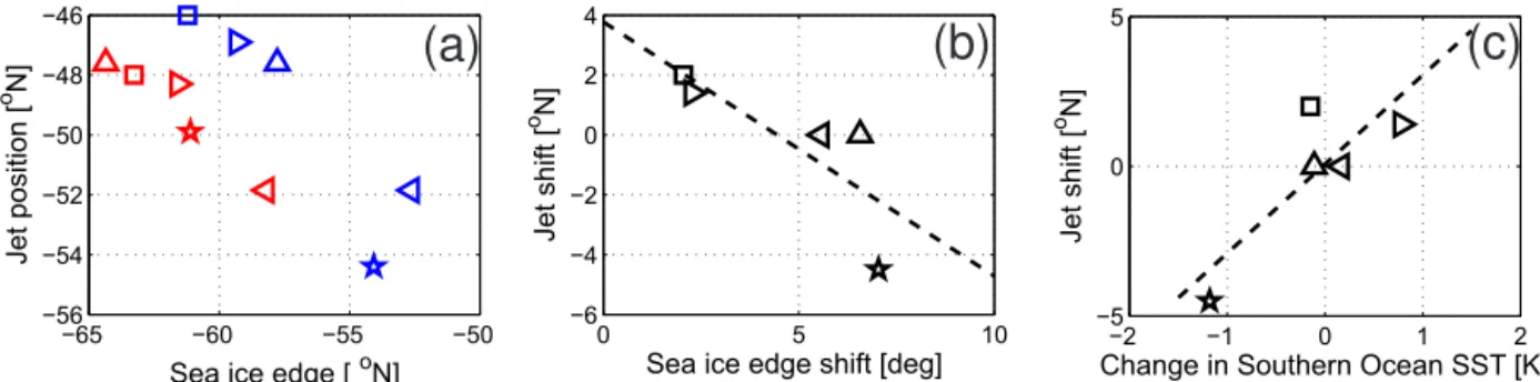
−65 −60 −55 −50 −56
−54 −52 −50 −48 −46
Sea ice edge [oN]
Jet position [
o N]
0 5 10
−6 −4 −2 0 2 4
Sea ice edge shift [deg]
Jet shift [
o N]
−2 −1 0 1 2
−5 0 5
Change in Southern Ocean SST [K]
Jet shift [
o N]
(c)
(b)
(a)
Figure 7.The relationship between sea ice, SST, and the position of the 850 hPa jet. Symbols represent individual models as shown in Fig. 2. All values are calculated using annual means. Red indicates the PI; blue indicates the LGM; and black indicates changes between the PI and the LGM (LGM−PI).(a)The jet position against sea ice extent (15 %),(b)jet shift against sea ice extent change, and(c)jet shift against Southern Ocean SST change. We use models where the PI jet position is poleward of 47◦S, and results are interpolated to the position of the Gersonde et al. (2005) observations before each calculation.
in the meridional temperature gradient. Given that LGM sea ice extended in the Atlantic and Indian sector close to 47◦S and in the Pacific sector to 57◦S (Gersonde et al., 2005), the key differences in jet shifts seem to be a dual function of state dependence and sea ice change.
All CMIP5-PMIP3 models show an LGM expansion of sea ice in the Southern Hemisphere, but there is consid-erable inter-model variability in the size of the expansion, which ranges from 2.1 and 7.0◦. State dependence (PI jet
position) and sea ice changes together control jet shift be-haviours. Only two models, CCSM4 and MRI-CGCM3, both simulate realistically large expansions in sea ice and sim-ulate PI jets which are south of 50◦S. These models show an increase in westerly wind speed around 55◦S and a large PI to LGM poleward shift in the jet in MRI-CGCM3. For models that have jets positioned relatively far to the south (at 48◦S±0.3◦) but do not correctly simulate the observed
expansion in sea ice, the resultant small polar atmospheric cooling causes little change in the meridional temperature gradient. In this case, westerly wind speed simply tends to weaken over the Southern Ocean latitudes. Models that sim-ulate a large increase in sea ice extent but have jets positioned too far towards the Equator are not sensitive to the LGM ex-pansion of sea ice: they show a slight weakening ofU, but
no jet shifts. The jet is not significantly affected by these sea ice increases, and associated meridional temperature gradient changes, because they happen too far poleward of the baro-clinic jet zone. This also fits with the study of Kidston et al. (2011), who found that whilst the jet will shift significantly poleward when the sea ice extent is substantially increased, there is little response if the sea ice edge is far from the jet.
We can generalise the relationship between sea ice extent and jet position. In models with accurately positioned PI jets, a 1◦difference in the sea ice edge tends to be associated with a−0.85◦shift in the 850 hPa jet. However, without any
ex-pansion in sea ice, it seems that the jet would shift towards the Equator, by around 4◦during the LGM. Thus we
tenta-tively conclude that around 5◦of sea ice expansion is neces-sary to hold the jet in its PI position. Given that data support a northward expansion of more than 5◦(Gersonde et al., 2005; Roche et al., 2012), this result does suggest that a slight pole-ward shift (and intensification) is likely to have been a feature of the LGM jet at 850 hPa. This fits with the findings of Sime et al. (2013), who found that cooling near the edge of the LGM Southern Ocean sea ice caused a wind intensification which is largest between 56 and 58◦S. However, we
empha-sise that these results only apply to CMIP5 models with jets that are relatively accurately positioned i.e. those which are sensitive to the impact of sea ice changes; if the model has a jet which sits equatorward of about 47◦S then the relation-ship breaks down. We note also that surface wind and shear stress changes may show different changes, so these results do not necessarily hold for all wind prognostics (Sime et al., 2013; Liu et al., 2015).
the impact of LGM sea ice counters and reverses the equa-torward trend in cooler climates so that the LGM winds were more likely to have also been shifted slightly poleward.
5 Data availability
Appendix A: Observational data and calculating model–data agreements
Acknowledgements. The work was funded by NERC grants NE.K004514.1 and NE/J004804/1 and also forms part of the British Antarctic Survey Polar Science for Planet Earth Programme. We acknowledge the support of the ARCHER UK National Supercom-puting Service (http://www.archer.ac.uk) and the World Climate Research Programme’s Working Group on Coupled Modelling, which is responsible for CMIP, and we thank the all the climate modelling groups for producing and making available their model output.
Edited by: H. Goosse
Reviewed by: three anonymous referees
References
Alexander, M. A., Bhatt, U. S., Walsh, J. E., Timlin, M. S., Miller, J. S., and Scott, J. D.: The Atmospheric Re-sponse to Realistic Arctic Sea Ice Anomalies in an AGCM during Winter, J. Climate, 17, 890–905, doi:10.1175/1520-0442(2004)017%3C0890:tartra%3E2.0.co;2, 2004.
Bracegirdle, T. J., Shuckburgh, E., Sallee, J.-B., Wang, Z., Mei-jers, A. J. S., Bruneau, N., Phillips, T., and Wilcox, L. J.: As-sessment of surface winds over the Atlantic, Indian, and Pacific Ocean sectors of the Southern Ocean in CMIP5 models: histor-ical bias, forcing response, and state dependence, J. Geophys. Res.-Atmos., 118, 547–562, doi:10.1002/jgrd.50153, 2013. Braconnot, P., Otto-Bliesner, B., Harrison, S., Joussaume, S.,
Pe-terchmitt, J.-Y., Abe-Ouchi, A., Crucifix, M., Driesschaert, E., Fichefet, Th., Hewitt, C. D., Kageyama, M., Kitoh, A., Laîné, A., Loutre, M.-F., Marti, O., Merkel, U., Ramstein, G., Valdes, P., Weber, S. L., Yu, Y., and Zhao, Y.: Results of PMIP2 coupled simulations of the Mid-Holocene and Last Glacial Maximum – Part 1: experiments and large-scale features, Clim. Past, 3, 261– 277, doi:10.5194/cp-3-261-2007, 2007.
Braconnot, P., Harrison, S. P., Kageyama, M., Bartlein, P. J., Masson-Delmotte, V., Abe-Ouchi, A., Otto-Bliesner, B., and Zhao, Y.: Evaluation of climate models using palaeoclimatic data, Nature Climate Change, 2, 417–424, doi:10.1038/nclimate1456, 2012.
Brayshaw, D. J., Hoskins, B., and Blackburn, M.: The Storm-Track Response to Idealized SST Perturbations in an Aquaplanet GCM, J. Atmos. Sci., 65, 2842–2860, doi:10.1175/2008jas2657.1, 2008.
Chavaillaz, Y., Codron, F., and Kageyama, M.: Southern westerlies in LGM and future (RCP4.5) climates, Clim. Past, 9, 517–524, doi:10.5194/cp-9-517-2013, 2013.
Chen, G., Plumb, R. A., and Lu, J.: Sensitivities of zonal mean at-mospheric circulation to SST warming in an aqua-planet model, Geophys. Res. Lett., 37, L12701, doi:10.1029/2010gl043473, 2010.
Denton, G. H., Anderson, R. F., Toggweiler, J. R., Edwards, R. L., Schaefer, J. M., and Putnam, A. E.: The Last Glacial Termi-nation, Science, 328, 1652–1656, doi:10.1126/science.1184119, 2010.
d’Orgeville, M., Sijp, W. P., England, M. H., and Meissner, K. J.: On the control of glacial-interglacial atmospheric CO2variations by the Southern Hemisphere westerlies, Geophys. Res. Lett., 37, L21703, doi:10.1029/2010gl045261, 2010.
Ferrari, R., Jansen, M. F., Adkins, J. F., Burke, A., Stewart, A. L., and Thompson, A. F.: Antarctic sea ice control on ocean circu-lation in present and glacial climates, P. Natl. Acad. Sci. USA, 111, 8753–8758, doi:10.1073/pnas.1323922111, 2014.
Gersonde, R., Crosta, X., Abelmann, A., and Armand, L.: Sea surface temperature and sea ice distribution of the last glacial. Southern Ocean – A circum-Antarctic view based on siliceous microfossil records, Quaternary Sci. Rev., 24, 869–896, 2005. Hodgson, D. A. and Sime, L. C.: Palaeoclimate: Southern westerlies
and CO2, Nat. Geosci., 3, 666–667, doi:10.1038/ngeo970, 2010. Kidston, J. and Gerber, E. P.: Intermodel variability of the poleward shift of the austral jet stream in the CMIP3 integrations linked to biases in 20th century climatology, Geophys. Res. Lett., 37, L09708, doi:10.1029/2010gl042873, 2010.
Kidston, J., Taschetto, A. S., Thompson, D. W. J., and England, M. H.: The influence of Southern Hemisphere sea-ice extent on the latitude of the mid-latitude jet stream, Geophys. Res. Lett., 38, L15804, doi:10.1029/2011GL048056, 2011.
Kim, S., Flato, G., and Boer, G.: A coupled climate model simula-tion of the Last Glacial Maximum, Part 2: approach to equilib-rium, Clim. Dynam., 20, 635–661, 2003.
Kohfeld, K. E., Quere, C. L., Harrison, S. P., and Anderson, R. F.: Role of Marine Biology in Glacial-Interglacial CO2Cycles, Sci-ence, 308, 74–78, doi:10.1126/science.1105375, 2005.
Kohfeld, K. E., Graham, R. M., de Boer, A. M., Sime, L. C., Wolff, E. W., Le Quéré, C., and Bopp, L.: Southern Hemi-sphere westerly wind changes during the Last Glacial Maximum: paleo-data synthesis, Quaternary Science Reviews, 68, 76–95, doi:10.1016/j.quascirev.2013.01.017, 2013.
Lamy, F., Gersonde, R., Winckler, G., Esper, O., Jaeschke, A., Kuhn, G., Ullermann, J., Martinez-Garcia, A., Lambert, F., and Kilian, R.: Increased Dust Deposition in the Pacific South-ern Ocean During Glacial Periods, Science, 343, 403–407, doi:10.1126/science.1245424, 2014.
Lee, S.-Y., Chiang, J. C. H., Matsumoto, K., and Tokos, K. S.: Southern Ocean wind response to North Atlantic cooling and the rise in atmospheric CO2: Modeling perspective and pa-leoceanographic implications, Paleoceanography, 26, PA1214, doi:10.1029/2010pa002004, 2011.
Liu, W., Lu, J., Leung, Xie, S.-P., Liu, Z., and Zhu, J.: The de-correlation of westerly winds and westerly-wind stress over the Southern Ocean during the Last Glacial Maximum, Clim. Dy-nam., 45, 3157–3168, doi:10.1007/s00382-015-2530-4, 2015. MARGO Project Members: Constraints on the magnitude and
patterns of ocean cooling at the Last Glacial Maximum, Nat. Geosci., 2, 127–132, doi:10.1038/ngeo411, 2009.
Menviel, L., Timmermann, A., Mouchet, A., and Timm, O.: Cli-mate and marine carbon cycle response to changes in the strength of the Southern Hemispheric westerlies, Paleoceanography, 23, PA4201, doi:10.1029/2008PA001604, 2008.
MITgcm Group: MITgcm user manual, online documentation, Tech. rep., MIT-EAPS, Cambridge, USA, 2013.
Otto-Bliesner, B. L., Brady, E., Clauzet, G., Thomas, R., Levis, S., and Kothavala, Z.: Last glacial maximum and Holocene climate in CCSM3, J. Climate, 19, 2526–2544, 2006.
Rojas, M.: Sensitivity of Southern Hemisphere circulation to LGM and 4×CO2 climates, Geophys. Res. Lett., 40, 965–970, doi:10.1002/grl.50195, 2013.
Sigman, D. M., Hain, M. P., and Haug, G. H.: The polar ocean and glacial cycles in atmospheric CO2 concentration, Nature, 466, 47–55, doi:10.1038/nature09149, 2010.
Sime, L. C., Kohfeld, K. E., Le Quéré, C., Wolff, E. W., de Boer, A. M., Graham, R. M., and Bopp, L.: Southern Hemisphere westerly wind changes during the Last Glacial Maximum: model-data comparison, Quaternary Sci. Rev., 64, 104–120, doi:10.1016/j.quascirev.2012.12.008, 2013.
Swart, N. C. and Fyfe, J. C.: Observed and simulated changes in the Southern Hemisphere surface westerly wind-stress, Geophys. Res. Lett., 39, L16711, doi:10.1029/2012gl052810, 2012. Taylor, K. E., Stouffer, R. J., and Meehl, G. A.: An Overview of
CMIP5 and the Experiment Design, B. Am. Meteorol. Soc., 93, 485–498, doi:10.1175/bams-d-11-00094.1, 2011.
Toggweiler, J. R., Russell, J., and Carson, S. R.: Midlatitude west-erlies, atmospheric CO2, and climate change during the ice ages, Paleoceanography, 21, PA2005, doi:10.1029/2005PA001154, 2006.
Tschumi, T., Joos, F., and Parekh, P.: How important are Southern Hemisphere wind changes for low glacial car-bon dioxide? A model study, Paleoceanography, 23, PA4208, doi:10.1029/2008pa001592, 2008.
Völker, C. and Köhler, P.: Responses of ocean circulation and car-bon cycle to changes in the position of the Southern Hemi-sphere westerlies at Last Glacial Maximum, Paleoceanography, 28, 726–739, doi:10.1002/2013pa002556, 2013.