Maria Christina de Souza Galvão*, João Ricardo Sato**, Edvaldo Capobiango Coelho***
Dahlberg formula – a novel approach
for its evaluation
Introduction: The accurate evaluation of error of measurement (EM) is extremely important as in growth studies as in clinical research, since there are usually quantitatively small changes. In any study it is important to evaluate the EM to validate the results and, consequently, the conclusions. Because of its extreme simplicity, the Dahlberg formula is largely used worldwide,
mainly in cephalometric studies. Objectives: (I) To elucidate the formula proposed by Dahlberg
in 1940, evaluating it by comparison with linear regression analysis; (II) To propose a simple methodology to analyze the results, which provides statistical elements to assist researchers in
obtaining a consistent evaluation of the EM. Methods: We applied linear regression analysis,
hy-pothesis tests on its parameters and a formula involving the standard deviation of error of
mea-surement and the measured values. Results and Conclusion: we introduced an error coefficient,
which is a proportion related to the scale of observed values. This provides new parameters to facilitate the evaluation of the impact of random errors in the research final results.
Abstract
Keywords: Biostatistics. Dahlberg error. Method error. Linear regression analysis.
* MSc in Dentistry, Methodist University of São Paulo (UMESP). Student, Specialization Course in Applied Statistics, UMESP. ** Professor, Lato-Sensu Specialization Course in Applied Statistics, UMESP.
*** MSc in Statistics, University of São Paulo. Head of the Lato-Sensu Specialization Course in Applied Statistics, UMESP. INTRODUCTION
In biological research, it is not often pos-sible to assess quantitative measurements di-rectly from living beings. Therefore, indirect methods are used and it is necessary to evaluate their effectiveness when compared with other methods. It is not possible to state which one is more accurate, but it is feasible to compare
the agreement levels. The standard method is usually called “Gold Standard”, however, this
does not mean that there is no error.1 The
ran-domized sample is one of the most important approaches to reduce bias. In another way, measure replications can be a good method to quantify and control random errors. The results of a trial might not be reliable if no
» The authors report no commercial, proprietary, or inancial interest in the products or companies described in this article.
How to cite this article: Galvão MCS, Sato JR, Coelho EC. Dahlberg
satisfactory control of the error of
measure-ments was performed.6
In dentistry, in order to interpret the results of a study, the author has to consider how im-precise it is to trace landmarks. In both studies of growth and in clinical trials, the changes are subtle, which makes the error of the method
quite important.7 In order to evaluate the
vari-ance of error between researches, several
au-thors4,6,7,8,10 suggested the formula proposed
by Dahlberg6 in 1940. This method assumes
that the sample has a normal distribution and,
mainly, there is no bias (systematic error).6
Furthermore, the connections between er-ror of measurement (EM) and misinterpreta-tion of the results were not menmisinterpreta-tioned. In any research project, it is important to reduce the EM as much as possible, mainly when changes in measures were small comparing with the original scale of data. This wariness allows that the results, and consequently, the conclusions,
can be validated.7
There is almost no reference to decide if some amount of error can be considered accept-able or not. In several papers the interpretation of the result is empirical or it is based on the personal experience of the investigator.
Accord-ing to Midtgard, Bjork, Linder-Aronson9 and
Battagel,3 the error of variance should be
ide-ally less than 3% of the total variance. However,
Midtgard, Bjork and Linder-Aronson9 stated
that it is almost impossible to have a variance of error less than 10% of the total variance.
Ba-umrind and Frantz2 reported that differences of
measures derived from a patient should be at least the double of the standard deviation of the error of measurement. In this way, they can be considered as treatment results.
Although several studies reported few changes during a treatment, it is important to evaluate these changes properly. EM can be re-duced but not totally eliminated. If therapeu-tic changes were small, EM can significantly
influence the inference of the evaluated differ-ences. Therefore, there is a need to elaborate methodologies to analyze and interpret the ef-fects of the EM in the changes observed during the treatment. Actually, there is no agreement
about this subject in the literature.7
Regression analysis allows the assessment of systematic and random errors. It also permits a very intuitive visual evaluation of the results through a scatter plot chart and an optimum fit-ted line to these points. Further information about regression analysis can be found in the study of
Wackerly, Mendenhall III and Scheaffer.11
Due to it’s simplicity, the Dahlberg formula is frequently applied in dental research, in spite of other methods and different approaches to analyze the error, such as the one proposed by
Martelli Filho et al.8 The aims of this paper
were: To interpret the meaning of the Dahlberg6
formula proposed in 1940, to compare it to lin-ear regression analysis and to propose a simple method to analyze the results of this formula.
MATERIAL AND METHODS
For the EM study, data sets of masters thesis in dentistry were kindly provided by their authors.
Data sets
1) From an initial sample of 20 orthodontic dental casts, the lingual shape of the arch was evaluated by using X and Y coordinates, result-ing in 40 coordinates. Ten were re-measured to
evaluate the EM.12
2) This study was based on 17 adult pa-tients under orthodontic treatment, whom had magnetic resonance imaging taken in three different occasions. The tipping of an-terior teeth (canine to canine) was measured
using the author’s own method.4 From these
Methods for error analysis
Dahlberg formula
The Dahlberg6 formula is defined as:
∑
=
=
N
i i
N
d
D
1 2
2
di is the difference between the first and the
second measure, and N is the sample size which was re-measured.
Assume the model Zij=ui+εij where i is the sam-ple index (i=1,2,3,...,N), j is the measure index (1st measure, 2nd measure), Z
ij is the observed measure, ui is the actual measure and εij the EM.
Regarding the EM, it is assumed that the
ex-pectation is E(εij)=0and the variance VAR(εij)=δ2 ε.
Thus, one probable quantification of the EM is its respective standard deviation εij, or, δε. In oth-er words, the smalloth-er the standard deviation the smaller will be the error of method.
Observing the difference between the second and the first measure, we have:
di=Zi2-Zi1
so
Var (di)=Var (εi2-εi1)=2δ2
ε
In this way, if we assume that there is no bias (systematic error), one intuitive estimator for 2δ2
ε could be:
2δ2
ε=Σ di2/N
and therefore,
δz
ε=Σ di2/2N
Thus, the quantity
∑
=
=
N i
i
N d
1 2
2 ˆ
ε
δ
is exactly the formula Dahlberg proposed in 1940. This estimator of standard deviation of the EM is largely used in orthodontic research and gives us the root of the mean squared error (SSE), being equivalent to standard deviation of
this error in case of no bias (systematic error),6
i.e., if the mean of errors is equal to zero. Note that Dahlberg error is extremely sensi-tive to bias, since any mean deviation between the two measures will be incorporated. Besides, the Dahlberg formula presumes equality, not only between the means of the first and sec-ond measures but also of their variances. This second kind of systematic error, named “bias of slope”, will be more detailed in the next section. In summary, Dahlberg error does not distinguish between systematic and random er-rors, making it difficult to interpret the results.
Regression model
Several biological phenomena can be ex-plained by mathematical models. Regression anal-ysis describes a straight line as a relation function between two variables in a set of data. It is neces-sary to find the best line to fit this relation. The equation of the line is:
Y=β0+β1X
β0 is the intercept (value of Y when the line
crosses the X axis) and β1 is the slope coefficient of the line.
For a linear regression model, it includes a ran-dom error, and thus, we have:
50 45 40 35 30 25 20 15 10 5 0
25 20
15 10
5 0
25
25 20
20 15
15 10
10 5
5 0
0
where ni has mean zero and variance δ2
n. Details about the estimation process and test of hypothesis for parameters β0 and β1 can be found in the study
of Wackerly, Mendenhall III and Scheaffer.11
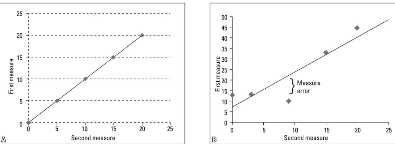
For dentistry, considering Yi and Xi as the val-ues for the i-th sample at first and second measures (i.e., Yi=Zi1 and Xi=Z21), the case without any bias or EM occurs if β0= 0, β1= 1 and δ2
n= 0. One illustra-tive example of this case is in Figure 1A, in which a straight line has fitted perfectly to the points.
In Figure 1B, the points do not fit perfectly to the straight line. In this case there are scat-tered points along the line, indicating the pres-ence of EM. In this case, the best fit in the least-squares criterion minimizes the sum of squared residuals. Residual is the vertical dis-tance between the observed point and the
fit-ted line.11 Note also that the fitted line does
not cross the origin, i.e., β0 is different of zero, showing a bias in the mean of the error. It can be also noticed in Figure 1B that the inclina-tion of the line is not 45º, which means that
there is a slope bias, i.e., β1 is different of 1.
These two types of systematic errors can occur at the same time or not, and this Figure is only for illustrative purposes.
In practice, due to random fluctuations, the
estimation of β0 and β1 coefficient will hardly
be equal to one and zero, respectively. Thus, it is necessary to perform statistical tests to detect systematic errors. In these cases, t-statistics of es-timators5 of β
0 and β1 can be used, testing the null hypothesis for β0= 0 (mean bias) and β1=1 (slope bias), respectively. These measures come from regression analysis and can be found in the study
of Wackerly, Mendenhall III and Scheaffer.11
If there is no systematic error, then Zi1 can be written as Zi1=Zi2+ni.
Moreover, as Zi2=µi+εi2, we have
µi+εi2+ni=µi+εi1, then εi1=εi2+ni and, so, ni=εi1-εi2,
being εi1= first measure error and εi2= second
measure error. As,
2 1 2
2
2
)
(
)
(
)
(
ε
ε
δ
εδ
n=
Var
n
i=
Var
i+
Var
i=
, then2
22
δ
nδ
ε=
being δ2
n the error of variance of the regression
analysis, which the estimator is denoted by δ2
n.
FIGURE 1 - A) 45 degree slope regression line fitted to the points. B) Regression line with mean bias, inclination and EM. Second measure
First measure
Measure error
Second measure
First measure
By calculating the square root of this coeffi-cient, we have a measure equivalent to Dahlberg error, i.e.,
2
ˆ
n
δ
δ
ε=
Despite this, the formula will only be valid in case of no slope bias. One general formula in cases with systematic errors is given by:
. ˆ 1
ˆ
2 1
β
δ
δ
ε+
= n
Evaluation of found errors
If we assume that any distance can be de-scribed as the true distance plus an error, which has a Gaussian distribution, we have:
Z1i=µi+ε1i and Z2i=µi+ε2i where εi~N(o,δ2
ε).
From the statistics theory, we know that 95% of the data from one randomized sample with normal distribution have the mean between µi-1,96 δ2
ε and
µi+1,96 δ2
ε. Thus,
) ˆ 1,96 ˆ
1,96 ( 2
1
1 2
1 1
∑
∑
= =
+ =
N
i i
N
i Zi Z
N
P δε δε
where N = is the number of data re-measured,
δε = standard deviation estimator of the EM.
Z1i = first measure,
Z2i= second measure.
This indicates that the ratio between EM and the observed measures is smaller than P in approximately 95% of the sample. Note that P is a proportion of the error related to the mea-sured value, i.e., a percentage. This property makes it easier to interpret the results, since the reliability can be expressed in terms of a
pro-portion (i.e., 10%, 25%, etc). Note the original Dahlberg formula does not use this feature as it does not consider the total value of the original measures, but just the difference between them. The same absolute value of error in a sample with small measures has greater influence than in one with big measures.
RESULTS
The first set of data and their results are shown in Table 1 and 2 and Figure 2.
In approximately 95% of the cases the EM is in average less than 0.69% of the value from the observed measures. Note that under a significance level of 5% (Type I error) there is no mean (p-value=0.820) or slope (p-value=0.775) bias.
For the second set of data, the observed mea-sures are shown in Table 3 and 4 and the results in Table 5 and Figure 3.
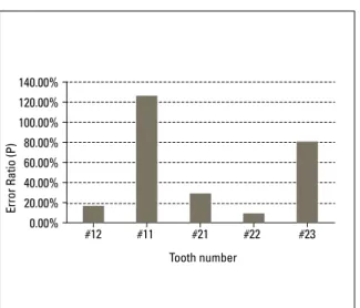
In this case, the error ratio (P) ranged from 9.38% to 125.88%. The biggest error ratio was found in tooth #11 and the smaller in tooth #22. Analyzing the systematic error test under
a significance level of 5% (β0=0 and β1=1), it
can be concluded that there were mean (p-value=0.029) and slope (p-value=0.043) bias for tooth #23.
DISCUSSION
The formula proposed by Dahlberg6 in 1940
assumes no systematic error in mean (β0) or in
slope (β1). Nevertheless, the results obtained
through regression analysis do not require these assumptions. Moreover, it also allows an intuitive analysis of the error using a scatter plot chart and a fitted line as shown in Figure 2. This scatter plot
chart can be easily built with a Microsoft Excel®
41 40 39 38 37 36 35 34 33 32 31
34 35 36 37 38 39 40 41
X1 X2 d d2
37.44 37.36 -0.08 0.0064 35.5 35.79 0.29 0.0841 37.02 37.06 0.04 0.0016 40.47 40.3 -0.17 0.0289
36.82 36.82 0 0
36.01 35.98 -0.03 0.0009 34.61 34.32 -0.29 0.0841 39.44 39.39 -0.05 0.0025 37.17 36.84 -0.33 0.1089 39.29 39.13 -0.16 0.0256
TABLE 1 - Dahlberg error formula6. TABLE 2 - Comparison between the results of the Dahlberg formula6 and
Regression Analysis. P is the percentage of calculated error
Systematic Error Test: (1) = mean bias; (2) = slope bias; A = paired t-test.
Error Estimated β 0
p-value (1)
Estimated
β1
p-value (2)
Dahlberg 0.131 - 0.197A -
-Regression 0.131 -0.299 0.820 1.01 0.775
P 0.691%
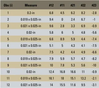
TABLE 3 - Second set of data: first measure Zi1 (# = tooth number). Obs (i) Measure #12 #11 #21 #22 #23
1 0.2-in 6.8 4.5 6.2 8.2 -2.8 2 0.019 x 0.025-in 9.4 0 2.4 6.7 -1 3 0.021 x 0.025-in 9.6 2.8 3.3 6.9 -0.9 4 0.02-in 5.8 6 5 4.8 -5.6 5 0.019 x 0.025-in 6.6 8.9 5.9 4.4 -7.4 6 0.021 x 0.025-in 5.1 5 4.3 4.1 -7.5 7 0.02-in 7.5 4.2 4.4 4.9 -6.6 8 0.019 x 0.025-in 7.9 5.9 5.7 4.7 -8.2 9 0.021 x 0.025-in 10 7.8 5.3 5.6 -10 10 0.02-in 12.4 16.8 16.6 11 -0.9 11 0.019 x 0.025-in 18.1 18 15.1 13.2 -2.1 12 0.021 x 0.025-in 14 15.5 11.6 9.5 -3.1
TABLE 4 - Second set of data: second measure Z2l (# = tooth number). Obs (i) Measure #12 #11 #21 #22 #23
1 0.02-in 7.8 0.1 4.8 8.4 -1.1 2 0.019 x 0.025-in 11.4 0 3.2 6.7 -1.5 3 0.021 x 0.025-in 10.6 2.9 3.7 6.7 -0.6 4 0.02-in 5.2 4.1 3.9 4.2 -6.8 5 0.019 x 0.025-in 5.5 6.9 4.4 4.4 -7.9 6 0.021 x 0.025-in 4.8 6.1 4.1 4.2 -7.4 7 0.02-in 8.7 4 5.9 5.3 -7.1 8 0.019 x 0.025-in 8.8 5 5.9 5.1 -6.5 9 0.021 x 0.025-in 10.2 7.1 7.3 6.7 -10.2 10 0.02-in 12.6 17.1 18 11.2 1.8 11 0.019 x 0.025-in 17.1 17.6 16.6 13.6 -0.5 12 0.021 x 0.025-in 14.7 14.3 12.5 9.7 -3.9
FIGURE 2 - Sample 1 – Regression line.
First measure
Second measure Data set 1 TABLE 5 - Results using Dahlberg6 formula, Paired t-test, Regression
Analysis and P ratio.
#12 #11 #21 #22 #23
Dahlberg Error 0.692 1.141 0.856 0.304 0.880 EM
(regression) 0.713 1.051 0.794 0.296 0.819 p-value
paired t-test 0.230 0.064 0.303 0.146 0.329 Beta 0 -0.006 1.344 0.579 0.076 -1.195 p-value to
mean bias 0.995 0.067 0.318 0.816 0.029 Beta 1 0.965 0.930 0.873 0.964 0.808 p-value to
in comparison to the observation sizes (P=0.69%). Moreover, using regression analysis we observed that β0 is statistically equal to zero (p-value=0.820) and β1 is equal to 1 (p-value=0.775). Therefore, we can conclude that there is no evidence of mean or slope biases and, when this happens, the EM estimated by the Dahlberg formula or regression analysis are very close, as shown in Table 2.
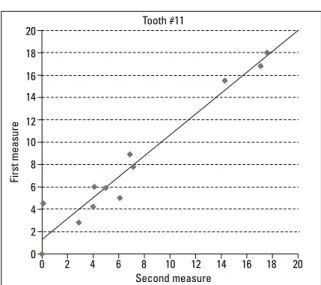
In sample 2, we analyzed the teeth with small measurement error (Fig 4) and those with the big-gest error (Fig 5). We can visualize, by comparing the points in Figure 5, that the points did not fit the line as in Figure 4. The results of Trpkova et al10 demonstrated that there is a systematic error and a random error involving the tracing of the land-marks. There is a standard mean error and a con-fidence interval of 95% in repetition and repro-duction of 15 landmarks regularly used in facial growth analysis. An average error of 0.59 mm on X axis and 0.56 mm on Y was considered ac-ceptable accuracy, even though this criteria did not take into consideration the total scale of the measure. Other researchers proposed to evaluate the variance of error. Midtgard, Bjork,
Linder-Ar-onson9 and Battagel3 stated that variance should
be ideally less than 3% of the total variance.
But, in a later paper, Midtgard, Bjork,
Linder-Aronson9 reported that it was almost impossible
to have a variance of error of less than 10% of the total variance. The use of analysis of vari-ance is quite complicated for researches who are not familiar to the intricacies of statistics. Maybe this is why the Dahlberg formula is so broadly used, mainly in studies using cephalo-metric measures. The Dahlberg formula lacks bias analysis, which makes it hard for research-ers to be secure if the error is acceptable or not. When we evaluated the values on Table 5, we can clearly notice that the analysis of the abso-lute value given by Dahlberg formula did not give us the parameters to evaluate the amount of error made. In tooth #21, the value provided by the formula was 0.856 and it corresponded to an error percentage of 29% (Fig 3). Mean-while, in tooth #23, we had a very similar value of 0.880, which corresponded to a percentage error of 81% (Fig 3). Thus, it is necessary to analyze the Dahlberg formula using parameters that permits one evaluation of the amount of
error made.By calculating the percentage of the
error in relation to the magnitude of the origi-nal measure, we were establishing a probabilis-tic limit to the error with 95% of confidence. In the second set of data, using regression analysis, we could evaluate the existence of mean and slope biases. From the analysis of Table 5, we can notice there were no bias neither in the measure with the lowest error nor in the one with the highest error. In this case, we can also verify that Dahlberg formula was very similar to the result of regression analysis in the low-est error case (tooth #22), with a difference of 0.008 between this values. It is interesting to mention that there was a tendency of slope bias in tooth #11 (p-value=0.065) and there were mean and slope biases in tooth #23 (Fig 6). These two teeth were the ones who had the biggest difference between the EM given by the Dahlberg formula and the regression method,
FIGURE 3 - P ratio for the second data set. Tooth number
Error Ratio (P)
140.00% 120.00% 100.00% 80.00% 60.00% 40.00% 20.00% 0.00%
4 6 8 10 12 14 4
6 8 10 12 14
0 2 4 6 8 10 12 14 16 18 20 0
2 4 6 8 10 12 14 16 18 20
0
0 -2 -4 -6 -8 -10 -12 -10 -8 -6 -2
-4
-12 2
showing that systematic error significantly influ-enced the Dahlberg formula. In these cases the Dahlberg formula differed from the regression analysis, mainly due to not making a difference between random and systematic error.
As the test for β0 and β1 referred to systematic er-ror, these biases can be numerically rectified depend-ing on the objective of the study. In several stud-ies, the mean bias can be explained by equipment
calibration problems or operator subjectivity. Nev-ertheless, the cause of slope bias is not very clear and can be related to errors in data collection process. It is important to highlight that the estimator and test of hypothesis referring to β1 had some limita-tions that were intrinsic to the estimation process. These procedures were suitable to a small set of ob-servations and with EM reasonably low. In fact, this is what usually occurs, as the re-measures are made only in a few samples and elevated EM can be easily detected and these samples discarded.
Besides, paired t-test commonly used to detect mean bias showed to be ineffective. In tooth #23, the paired t-test did not reveal statistically signifi-cant differences between the mean of the first and second measures, which were detected by regres-sion analysis as we can see in Table 5.
Baumrind and Frantz2 mentioned that the
dif-ferences observed in a patient must be at least two times the standard deviation of the estimated er-ror, so it can be considered as therapeutic results. This proposition of evaluating the ratio of the er-ror in relation to the measure lead to a less sub-jective parameter, which helps the researchers to determine what can be considered an acceptable error. However, the boundary value will depend on the accuracy level demanded by the research.
FIGURE 4 - Data set 2: Regression line adjusted to the data of tooth #22.
First measure
Second measure Tooth #22
FIGURE 5 - Data set 2: Regression line adjusted to the data of tooth #11.
First measure
Second measure Tooth #11
FIGURE 6 - Data set 2: Regression line adjusted to the data of tooth #23, which showed mean and slope biases.
First measure
CONCLUSION
The use of regression models to evaluate EM have some advantages: 1) It distinguishes system-atic error (mean and slope biases) from random error; 2) The results can be interpreted in a more objective and intuitive terms and permits a visual analysis using scattered plot charts and fitted line; 3) It supplies an estimation of EM integrated to the mathematical model.
The Dahlberg error is an estimator of stan-dard deviation of the EM and correspond to the estimated error by regression analysis, when there is no systematic error. This fact is not highlighted very often in the literature. Howev-er, when there were biases, the Dahlberg error was different to the one obtained by our analy-sis as demonstrated by our results.
Although the Dahlberg formula can be a sim-ple and efficient way to evaluate the EM, the anal-ysis of quality of measure using standard deviation is quite hard. The transformation of the given val-ue of this formula in a percentage of the amount measured provides parameters that makes it eas-ier to evaluate the impact of the random error in the final result of the research.
Contact address
João Ricardo Sato
Rua Santa Adélia, 166 – Bangu
Zip code: 05.056-020 – Santo André/SP, Brazil E-mail: [email protected]
1. Bland JM, Altman DG. Measuring agreement in method comparison studies. Stat Methods Med Res. 1999; 8(2):135-60.
2. Baumrind S, Frantz RC. The reliability of head ilm
measurements. Conventional angular and linear measurements. Am J Orthod. 1971;60(5):505-17. 3. Battagel JM. A comparative assessment of cephalometric
errors. Eur J Orthod. 1993;15(4):305-14.
4. Capelozza Filho L, Fattori L, Maltagliati LA. A new method to evaluate teeth tipping using computerized tomography. Rev Dental Press Ortod Ortop Facial. 2005;10(5):23-9. 5. Callegari-Jacques SM. Bioestatística. Princípios e aplicações.
Porto Alegre: Artmed; 2004.
6. Houston WJB. The analysis of errors in orthodontic measurements. Am J Orthod. 1983 May;83(5):382-90.
7. Kamoen A, Dermaut L, Verbeeck R. The clinical signiicance
of error measurement in the interpretation of treatment results. Eur J Orthod. 2001 Oct;23(5):569-78.
REfERENCES
8. Martelli Filho JA, Maltagliati LA, Trevisan F, Gil CTLA. Novo método estatístico para análise da reprodutibilidade. Rev Dental Press Ortod Ortop Facial. 2005;10(5):122-9. 9. Midtgård J, Björk G, Linder-Aronson S. Reproducibility
of cephalometric landmarks and errors of measurements of cephalometric cranial distances. Angle Orthod. 1974 Jan;44(1):56-61.
10. Trpkova B, Major P, Prasad N, Nebbe B. Cephalometric
landmarks identiication and reproducibility: a meta analysis.
Am J Orthod Dentofacial Orthop. 1997 Aug;112(2):165-70. 11. Wackerly DD, Mendenhall III W, Scheaffer RL. Mathematical
statistics with applications. 7th ed. California: Thomson
Brooks/Cole; 2008.
12. Yasushi IM. Estudo das formas e dimensões linguais das arcadas dentárias em indivíduos brasileiros com oclusão normal [dissertação]. São Paulo (SP): Universidade Metodista de São Paulo; 2007.
Submitted: July 7, 2008