Earth Syst. Dynam., 4, 109–127, 2013 www.earth-syst-dynam.net/4/109/2013/ doi:10.5194/esd-4-109-2013
© Author(s) 2013. CC Attribution 3.0 License.
Earth System
Dynamics
Open Access
Geoscientiic
Geoscientiic
Geoscientiic
Geoscientiic
Dynamical and biogeochemical control on the decadal variability
of ocean carbon fluxes
R. S´ef´erian1,2, L. Bopp2, D. Swingedouw2, and J. Servonnat2
1Centre National de Recherche de M´et´eo-France, CNRM-GAME – URA1357, 42 Avenue Gaspard Coriolis, 31100 Toulouse, France
2Laboratoire du Climat et de l’Environnement, LSCE – UMR8212, L’Orme des Merisiers Bˆat. 712, 91191 Gif sur Yvette, France
Correspondence to:R. S´ef´erian ([email protected])
Received: 26 November 2012 – Published in Earth Syst. Dynam. Discuss.: 21 December 2012 Revised: 8 March 2013 – Accepted: 21 March 2013 – Published: 9 April 2013
Abstract.Several recent observation-based studies suggest
that ocean anthropogenic carbon uptake has slowed down due to the impact of anthropogenic forced climate change. However, it remains unclear whether detected changes over the recent time period can be attributed to anthropogenic cli-mate change or rather to natural clicli-mate variability (inter-nal plus naturally forced variability) alone. One large uncer-tainty arises from the lack of knowledge on ocean carbon flux natural variability at the decadal time scales. To gain more insights into decadal time scales, we have examined the internal variability of ocean carbon fluxes in a 1000 yr long preindustrial simulation performed with the Earth Sys-tem Model IPSL-CM5A-LR. Our analysis shows that ocean carbon fluxes exhibit low-frequency oscillations that emerge from their year-to-year variability in the North Atlantic, the North Pacific, and the Southern Ocean. In our model, a 20 yr mode of variability in the North Atlantic air-sea carbon flux is driven by sea surface temperature variability and accounts for∼40 % of the interannual regional variance. The North Pacific and the Southern Ocean carbon fluxes are also charac-terised by decadal to multi-decadal modes of variability (10 to 50 yr) that account for 20–40 % of the interannual regional variance. These modes are driven by the vertical supply of dissolved inorganic carbon through the variability of Ekman-induced upwelling and deep-mixing events. Differences in drivers of regional modes of variability stem from the cou-pling between ocean dynamics variability and the ocean car-bon distribution, which is set by large-scale secular ocean circulation.
1 Introduction
In recent years, several observation-based and model-based studies have suggested that ocean anthropogenic carbon up-take has slowed down due to the impact of anthropogenic forced climate change in various ocean regions (e.g. Corbi`ere et al., 2007; Le Qu´er´e et al., 2007). However, the fact that these changes in ocean carbon fluxes are caused by anthro-pogenic forced climate change within the last decades is still debated (e.g. Ullman et al., 2009; McKinley et al., 2011).
Among these regions potentially impacted by anthro-pogenic forced climate change, the North Atlantic has been extensively studied over the three last decades (Watson et al., 2011; Schuster et al., 2009; Brown et al., 2010; Metzl et al., 2010; Corbi`ere et al., 2007; McKinley and Follows, 2004; McKinley et al., 2011). Debate prominently arises from dis-agreement between causes of trends in the North Atlantic carbon sink estimated from data or numerical model out-put. On the basis of in situ observations, several authors (i.e. Corbi`ere et al., 2007; Watson et al., 2011; Brown et al., 2010; Metzl et al., 2010) have reported a more rapid growth in surface ocean pCO2 than in atmospheric pCO2, which translates into a decline of the net ocean carbon uptake over the last decade. Possible mechanisms driving this de-cline are associated to climate-induced modifications of both oceanic and atmospheric dynamics, e.g., rising sea-surface temperature (Corbi`ere et al., 2007), increasing ocean stratifi-cation (Schuster et al., 2009) or changes in horizontal oceanic currents owing to a shift in the North Atlantic Oscillation (Thomas et al., 2007; Schuster et al., 2009). However, model
reanalysis studies, based on GFDL, CCSM and MIT ocean general circulation reanalyses, have demonstrated that the weakening of the North Atlantic carbon sink over the last three decades (i.e., 1970s to 2000s) cannot be really at-tributed to anthropogenic climate change, but rather to the natural variability of the ocean carbon sink driven by the North Atlantic Oscillation (McKinley et al., 2011; Thomas et al., 2008; L¨optien and Eden, 2010) as a part of the North-ern Annular Mode (NAM).
Similarly to the North Atlantic, many aspects of the South-ern Ocean dynamics and carbon cycle have exhibited trends over the last decades. Model simulations and inversions of atmospheric data have suggested that the southward shift of westerlies concomitantly with their strengthening had damp-ened the Southern Ocean carbon sink (e.g. Le Qu´er´e et al., 2007; Lovenduski and Ito, 2009). Such a response on ocean carbon fluxes has been highlighted by Lovenduski et al. (2008) on shorter time scales. In this study, authors demon-strated that the southward shift of westerlies associated with the positive trend in the Southern Annular Mode (SAM) could drive a weakening of the Southern Ocean carbon sink because of changes in water mass overturning. However, it seems that such a response of both water mass overturning and ocean carbon sink may be overstated at the decadal time scale since no changes in Southern Ocean circulation have been detected from observations, while these data detect co-herent warming and freshening trends in subsurface waters (Boening et al., 2008).
Therefore, from these previous studies, it remains unclear if detected changes in ocean carbon sink within the last decades can be attributed to anthropogenic climate change or to natural climate variability that is a combination of an internal variability and a naturally forced variability (related to volcanoes and solar forcings). One large uncertainty arises from the lack of knowledge on ocean carbon flux variability at decadal time scales (Bates, 2007; Takahashi, 2009).
So far, these time scales have been an active fields of re-search in the ocean dynamics community (e.g. Latif et al., 2006, and references therein). Studies generally agree to the fact that sea-surface temperature and other ocean variables exhibit low-frequency modes of variability within mid- and high latitude oceans (e.g. Latif et al., 2006; Zwiers, 1996; Boer, 2000, 2004). It is, thus, likely that the modes of vari-ability of the ocean carbon fluxes could be inherited from low-frequency modes of variability like the Atlantic Multi-decadal Oscillation (AMO; e.g. Bates, 2012; McKinley and Follows, 2004; McKinley et al., 2011), or the Pacific Decadal Oscillation (PDO; e.g., Valsala et al., 2012; Takahashi et al., 2006) in a similar way as their interannual variability is mainly associated with the tropical Pacific ocean variability caused by El Ni˜no and La Ni˜na (e.g. Chavez et al., 1999; Wang and Moore, 2012; McKinley and Follows, 2004).
However, studying low-frequency variations in ocean car-bon fluxes within these oceanic regions is not straight-forward. The major limitation comes from the temporal
coverage of the observations or model reanalysis. This lim-itation can be illustrated by considering the North Atlantic for investigating multi-year variations in ocean carbon fluxes (Ullman et al., 2009; L¨optien and Eden, 2010; Thomas et al., 2008). Here, large datasets (e.g. Gruber et al., 2002; Bakker et al., 2012) are available and ocean reanalysis are consis-tent over the 30 to 50 last years. Despite this large amount of information, an optimal spatial and temporal coverage of 30 to 50 yr provided by model reanalyses only allows study-ing 3 to 5 independent decades. Such limitation is, thus, even stronger for in situ observations. Observations are ei-ther combined and interpolated into large ocean regions in order to ensure a significant time sampling (McKinley et al., 2011), or merely considered in the terms of individual long-term stations (e.g. Gruber et al., 2002; Bates, 2007; Bates et al., 2012) that may be poorly representative of the basin-scale dynamics (McKinley and Follows, 2004).
In this context, long model simulations (>500 yr) are the only way to circumvent spatiotemporal sampling issues and have been demonstrated to include the minimum years of data to assess significantly variability at decadal time-scales (e.g. Boer, 2004). The usefulness of long model simulations for studying temporal variations of land and ocean carbon fluxes was first illustrated in Doney et al. (2006). Based on a 1000 yr fully coupled climate-carbon cycle simulation, the authors provide a good overview of the natural variability of the global carbon cycle in CCSM-1.4. However, in this study, both decadal and oceanic aspects receive less attention than the interannual variability of the terrestrial carbon cycle.
Here, as a first step to assess the internal decadal variabil-ity of the ocean carbon fluxes, we used an extended 1000 yr long preindustrial simulation performed with the Earth Sys-tem Model IPSL-CM5A-LR. Using output of this model sim-ulation, we performed several statistical time-series analyses to (i) track the low-frequency modes variability, (ii) locate the oceanic regions that contribute the most to these modes and (iii) identify the main drivers of the ocean carbon fluxes variability at decadal time scales.
2 Methodology
2.1 Model description and pre-industrial simulation
R. S´ef´erian et al.: Decadal variability of ocean CO2fluxes 111
Table 1.Description of the distinct ocean carbon fluxes (f gCO2) or oceanic partial pressure of carbon (pCO2) driven by the variability of
solely one driver (i.e., T/SST, S/SSS, DIC or Alk) compared to the fully-driven ocean carbon fluxes.
Alkalinity (Alk) Dissolved Inorganic Salinity (S) Temperature (T)
Carbon (DIC)
Fully-driven Interannual variability Interannual variability Interannual variability Interannual variability
Alk-driven Interannual Variability 1000 yr mean state 1000 yr mean state 1000 yr mean state
DIC-driven 1000 yr mean state Interannual Variability 1000 yr mean state 1000 yr mean state
S-driven 1000 yr mean state 1000 yr mean state Interannual Variability 1000 yr mean state
T-driven 1000 yr mean state 1000 yr mean state 1000 yr mean state Interannual Variability
is NEMOv3.2 (Madec, 2008). It offers a horizontal resolu-tion of 2◦refined to 0.5◦in the tropics and 31 vertical lev-els. NEMOv3.2 includes the sea ice model LIM2 (Fichefet and Maqueda, 1997), and the marine biogeochemistry model PISCES (Aumont and Bopp, 2006). PISCES simulates the biogeochemical cycles of carbon, oxygen and nutrients us-ing 24 state variables. Macronutrients (nitrate, ammonium, phosphate and silicate) and the micronutrient iron limit phy-toplankton growth and thus ensure a good representation of the high-nutrient low-chlorophyll regions (Aumont et al., 2003; Aumont and Bopp, 2006). Inorganic carbon pools are dissolved inorganic carbon, alkalinity and calcite. Total al-kalinity includes contributions from carbonate, bicarbonate, borate, hydrogen and hydroxide ions (practical alkalinity). For dissolved CO2 and O2, air-sea exchange follows the quadratic wind-speed formulation (Wanninkhof, 1992).
The core of this study is an extended preindustrial simu-lation of 1000 yr, in which the initial state of marine carbon cycle comes from a 3000 yr offline spinup plus 300 yr of on-line adjustment, while the dynamical components of IPSL-CM5A-LR have been spun-up for 600 yr (Dufresne et al., 2013). Spin-up strategy and model-data skill-assessment of (Dufresne et al., 2013). Spin-up strategy and model-data skill-assessment of IPSL-CM5A-LR’s modern state of ma-rine biogeochemistry are presented and discussed in S´ef´erian et al. (2013).
2.2 Analytical methodology
The goals and methodology of this study are twofold. First, we aim at tracking and quantifying low-frequency oscilla-tions of ocean carbon fluxes (here decadal to multi-decadal internal variability). For that purpose, we employ several statistical time-series analyses like the continuous wavelet transform (Torrence, 1998), the spectral density or the prin-cipal component analysis (PCA; Von Storch and Zwiers, 2002).
Secondly, we decipher which physical or biogeochemi-cal drivers (here alkalinity, dissolved inorganic carbon, salin-ity and temperature) control the various modes of variabil-ity of ocean carbon fluxes. We employ a decomposition of sea-waterpCO2(driving the ocean carbon fluxes) based on Takahashi et al. (1993) assuming that pCO2 is a function
of Alkalinity (Alk), dissolved inorganic carbon (DIC), salin-ity (S) and temperature (T): pCO2=f g(Alk, DIC, T, S). The variance of a function of several random variables is given by expanding the functionf (X1, X2, X3, . . . , Xn)
(herepCO2) in Taylor series around the mean values of X
(here considered as the 1000 yr yearly-averaged climatology of Alk, DIC,SandT):
Var(f (X1, X2, X3, ..., Xn))≈ n X
i=1
∂f ∂Xi
2
σX2 i
+ n X
i=1
n X
j6=i ∂f ∂Xi
∂f ∂Xj
Cov Xi, Xj
(1)
where σX2
i is the variance of the random variable Xi and
Cov(Xi, Xj) is the covariance between the random variables Xi andXj.
Based on this variance decomposition, we have conducted several offline computations of monthly-averaged sea-water
pCO2and ocean carbon fluxes in which only one ocean car-bon flux driver is allowed to vary in time while the others are fixed to their 1000 yr yearly-averaged climatology (Table 1). Online and offline computations of monthly-averaged sea-waterpCO2 and ocean carbon fluxes (f gCO2) show small differences in global average long-term mean and compare well in terms of variability (with a correlation ofR∼0.96).
Consequently, we assume that our variance decomposi-tion strategy allows us to single out the variance contribu-tion of Alk forpCO2-Alk orf gCO2-Alk, DIC for p CO2-DIC orf gCO2-DIC and so on. A similar approach was used in previous studies (e.g. Ullman et al., 2009; McKinley and Follows, 2004).
As described in Boer (2000, 2004), drifts in the variables matter for assessing low-frequency modes of variability. We have, therefore, removed drifts of ocean carbon fluxes and carbon-related fields, which have been estimated from lin-ear least-square regression in function of time for each vari-able. Yet, in our case drifts in sea-waterpCO2 and ocean carbon fluxes are small compared to the interannual or low-frequency oscillations: for global ocean carbon fluxes it rep-resents about−0.03 Pg C over 100 yr in the first century of the 1000 yr simulation and only−0.01 Pg C over 100 yr in the last century of the 1000 yr simulation.
a) Ocean carbon fluxes
Arctic Ocean
N. Atl. High−Lat
N. Atl. Mid−Lat
N. Atl. Low−Lat
N. Atl. Trop.
S. Atl. Trop.
S. Atl. Low−Lat
S. Atl. Mid−Lat
S. Sub−Polar. At.
Polar S. Ocean S. Sub−Pol. Pac Trop. Ind.
S. Ind. Mid−Lat
S.E. Pac. Mid−Lat
S.W. Pac. Mid−Lat
S.E. Pac. Trop. S.W. Pac. Trop.
N.E. Pac. Trop. N.W. Pac. Trop.
N.E. Pac. Low−Lat N.W. Pac. Low−Lat
N.E. Pac. High−Lat
ac. High−LatN.W
. P .
Carbon Flux (PgC y
−
1)
Arctic Ocean N. Atl. High−Lat
.
N. Atl. Mid−Lat
.
N. Atl. L ow−L
at
.
N. Atl. T rop.
S. Atl. T rop
.
S. Atl. Lo w−Lat
.
S. Atl. Mid−Lat
.
S. Sub−P olar
. At.
Polar S. OceanS. Sub−P ol. P
ac.
Trop . Ind.
S. Ind. Mid−Lat
.
S.E. P ac. Mid−Lat
.
S.W . Pac. Mid−Lat
.
S.E. P ac. T
rop.
S.W . Pac. T
rop.
N.E. P ac. T
rop.
N.W . Pac. T
rop.
N.E. P ac. L
ow−Lat
.
N.W . Pac. L
ow−Lat .
N.E. P ac. High−Lat
.
N.W . Pac. High−Lat
−0.4
−0.2
0.0
0
.2
0.4
Mikaloff et al., 2007 IPSL−CM5A−LR
b) Ocean carbon uptake
Atlantic
Southern
Ocean Indian Paciic
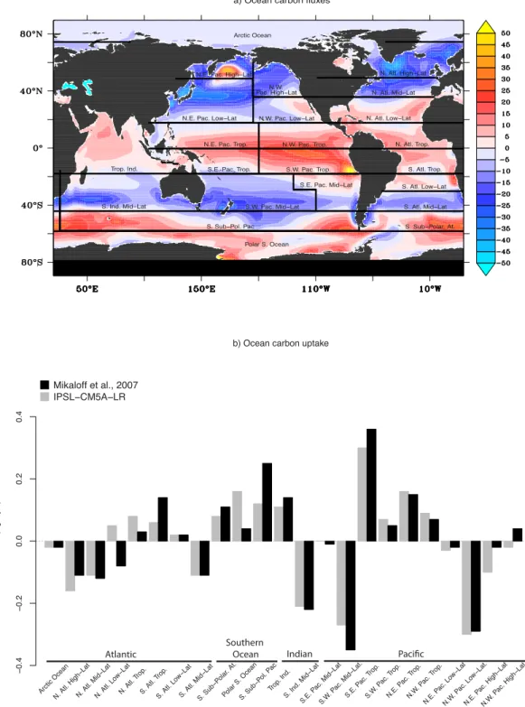
Fig. 1.Long-term mean of(a)simulated ocean carbon fluxes (in g C m−2yr−1) and(b)simulated regional carbon fluxes (in Pg C yr−1) compared to inversion-based estimates published in Mikaloff Fletcher et al. (2007). Black and grey bars indicate model and inversion-based estimates, respectively.
3 The preindustrial global ocean carbon fluxes
Hereafter, we present how the simulated carbon fluxes over the 1000 yr of preindustrial simulations compare to those es-timated from inverse modelling by Mikaloff Fletcher et al.
R. S´ef´erian et al.: Decadal variability of ocean CO2fluxes 113
0 200 400 600 800
−0.4
−0.2
0.0
0.2
0.4
Time [year]
Ocean Carbon Flux [PgC/y]
a) Detrended Global Carbon Flux
0 5 10 15 20 25 30
0.0
0.2
0.4
0.6
0.8
1.0
Time [year]
A
CF
b) Autocorrelation
Time [year]
P
er
iod [y
ear]
5 10 15 20 25
2
4
8
16
32
64
128
256
0 100 200 300 400 500 600 700 800 900 c) Wavelet Time−Frequency Spectrum
0 1 2 3 4 5 6 7
2
4
8
16
32
64
128
256
d) Wavelet Power Spectrum [(PgC y−1)2]
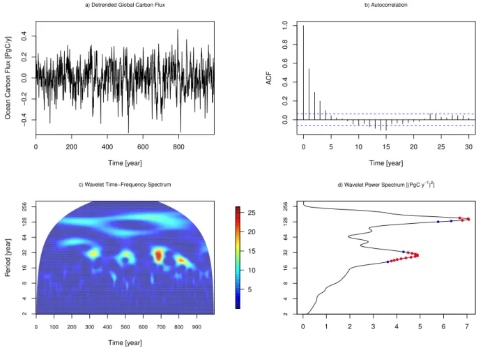
Fig. 2.Interannual time-series of the drift-corrected globally integrated ocean carbon flux (in Pg C yr−1) is represented in(a). The autocor-relation function(b), the wavelet time-frequency spectrum(c)and the averaged wavelet spectrum(d)describe the statistical properties of the drift-corrected global ocean carbon flux. A red noise hypothesis has been tested against the averaged wavelet spectrum. The significance of 95 % is mentioned with red points, while those of 90 % is mentioned in blue.
average. Regionally, the simulated oceanic sinks and sources of carbon agree with those estimated by inverse modelling with a global root-mean-square error of about 0.06 Pg C yr−1 (Fig. 1b). Only in the high latitude North West Pacific and the low latitude North Atlantic, simulated ocean carbon fluxes differ in sign from those estimated by inverse modelling. In the southern sub-polar regions, the model biases can be ex-plained by a shift of outgasing structures probably associated with the equator shift of main wind stress structures (Marti et al., 2009): compared to the inverse modelling-based esti-mates, our model simulates a stronger outgasing of carbon in the southern sub-polar Atlantic than in the polar Southern Ocean.
If we consider the time-variability over 1000 yr of the globally integrated ocean carbon flux in the preindustrial simulation, we can track low-frequency oscillations from its year-to-year variability (Fig. 2a). The 10 and 20 yr time-filtered (i.e., running mean) variances amount, respectively, to 0.08 and 0.05 Pg C yr−1 representing 56 and 37 % of the interannual variance (0.14 Pg C yr−1).
The imprint of low-frequency modes of variability on the global carbon flux can be diagnosed from the autocorrelation function (ACF) of the global ocean carbon flux (Fig. 2b). The shape of the ACF does not correspond to a first order autoregressive process (AR1), but rather to a third order au-toregressive process (AR3) according to the Yule-Walker es-timation (Von Storch and Zwiers, 2002). The fact that the ACF of the global ocean carbon flux cannot be mimicked by an AR1 indicates that long-term memory processes likely drive ocean carbon fluxes. This implies that the ocean carbon flux behaves as other oceanic variables, like sea-surface tem-perature or sea-surface salinity (Frankignoul, 1985), but its low-frequency variability has a strong imprint over several years.
Low-frequency modes of the global ocean carbon flux variability range within a time-window of about 128 to 200 yr (centennial mode) and 18 to 50 yr (decadal mode) as shown on the wavelet time-frequency diagram (Fig. 1c and d). In comparison to the centennial mode, the decadal mode is not continuously detected. Nevertheless, the wavelet power
spectrum within the decadal time-window is significantly stronger than a red noise wavelet spectrum (at 95 % in red dots, at 90 % in blue dots, Fig. 1d). The fact that the decadal mode appears sporadically over the time scales underlines the complexity of studying a globally integrated quantity, be-cause such a behaviour can be explained by a combination of several regional modes of variability either in phase or out of phase. As a consequence, in the next section, analyses will be conducted regionally.
4 Tracking the decadal mode of variability of regional
ocean carbon fluxes
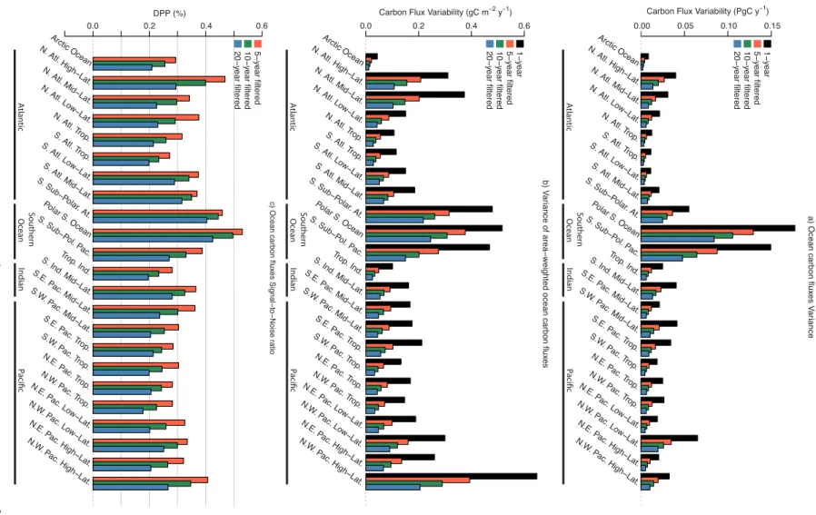
Modes of variability of one variable are an expression of its variance at several time scales. Here, the way we apprehend these different modes of variability, in a first approach, is to look at the variance of the time-filtered carbon fluxes in several oceanic regions, which correspond to those defined and used in Mikaloff Fletcher et al. (2007). The time filtering consists in a running mean of the regional carbon fluxes at 5, 10 and 20 yr (Fig. 3a). Except in the Arctic, the 1, 5 and 10 yr variances of the high latitude oceans are stronger com-pared to those found in mid- and low latitude regions. Yet, it is striking to see how the Southern Ocean variances (i.e., for all time filtering) dominate those of the other oceanic regions with a standard deviation of about 0.1 Pg C yr−1. Such differ-ences between the Southern Ocean and other oceanic regions are evidently fueled by differences in surface areas, which are much larger in the Southern Hemisphere regions than in the northern ones. As explained in Mikaloff Fletcher et al. (2007), region boundaries have been estimated using in situ measurements of1pCO2(Takahashi et al., 2002) and a gen-eral ocean circulation model, and have been designed con-sistently with TRANSCOM regions (Gurney et al., 2002). That is, each region differs greatly in surface area compared to each other. Therefore, surface area weighing allows com-paring the different regions independently of their design (Fig. 3b). Yet, variability of surface area weighted carbon fluxes is still much stronger in mid- and high latitude oceans than in the tropical ones.
In order to assess the relative importance of low-frequency modes of variability comparatively to interannual variability, we have employed a signal-to-noise ratio, the diagnosed po-tential predictability (DPP; Boer, 2004; Boer and Lambert, 2008; Persechino et al., 2013):
DPP= σ
2
M −
1
Mσ
2
σ2 (2)
where σ2 is the ocean carbon flux 1 yr variance and σM2
(M= 5, 10 and 20 yr) is the variance of the time-filtered ocean carbon flux.
The DPP metric (Fig. 3c) indicates that the 5 yr and the 10 yr time-filtered variances of ocean carbon fluxes within the North Atlantic, the North Pacific and the Southern Ocean
account, respectively, for more than 30 % of the 1 yr variance. The Southern Ocean is the only oceanic region where multi-decadal variability of ocean carbon fluxes (here represented by the 20 yr time-filtered variance) reaches up to 40 % of the 1 yr variance. These results are consistent with previous stud-ies showing that low-frequency variability of various climate variables is mainly located in the high latitude oceans (Boer, 2000, 2004; Persechino et al., 2013; Mauget et al., 2011).
In particular, the three oceanic regions are characterised by well understood modes of variability in ocean dynam-ical fields: the AMO for the North Atlantic (Kerr, 2000; Enfield et al., 2001), the PDO for the North Pacific (Mantua and Hare, 2002) and the signature of the Southern Annu-lar Mode on the Southern Ocean (Thompson and Wallace, 2000; Thompson et al., 2000). These various modes of ability have been suggested to have an influence on the vari-ability of ocean carbon fields (Bates, 2012; McKinley and Follows, 2004; McKinley et al., 2011; Valsala et al., 2012; Takahashi et al., 2006; Lenton and Matear, 2007; Lovenduski et al., 2008). However, the fact that the signal-to-noise ratio of ocean carbon fluxes are comparable with those of other cli-mate fields at regional scale with the same model (e.g., sea-surface temperature, sea-sea-surface salinity; Persechino et al., 2013) does not mean that the modes of variability or even the drivers are the same.
R. S ´ef ´erian et al.: Decadal v ariab ility of ocean CO 2 fluxes 115 −0.05 1−y ear 5−y ear filtered 10−y ear filtered 20−y ear filtered 1−y ear 5−y ear filtered 10−y ear filtered 20−y ear filtered
c) Ocean carbon flux
es Signal−to−Noise ratio
5−y ear filtered 10−y ear filtered 20−y ear filtered A tlantic S outhern Oc ean Indian P aciic
a) Ocean carbon flux
es V
a
riance
b) V
a
riance of area−weighted ocean carbon flux
es
Carbon Flux Variability (PgC y−1)
0.00 0.05 0.10 0.15
Carbon Flux Variability (gC m−2 y−1)
0.0 0.2 0.4 0.6
DPP (%)
0.0 0.2 0.4 0.6
Arctic Ocean N. Atl. High−Lat
. N. Atl. M
id−Lat. N. Atl. Lo
w−Lat . N. Atl. T
rop . S. Atl. T
rop . S. Atl. Lo
w−Lat . S. Atl. Mid−Lat
. S. Sub−P
olar. At.
Polar S. Ocean
S. Sub−P
ol. P ac. Trop
. Ind. S. Ind. M
id−Lat . S.E. P ac. Mid−Lat. S.W . P ac. Mid−Lat. S.E. P ac. T rop. S.W . P ac. T rop . N.E. P ac. T rop . N. W.
Pac. T
rop . N.E. P ac. Lo w−Lat . N.W . P ac. Lo w−Lat . N.E. P ac. High−Lat. N.W . P ac. High−Lat . A tlantic S outhern Oc ean Indian P aciic Arctic Ocean N. Atl. High−Lat
. N. Atl. M
id−Lat. N. Atl. Lo
w−Lat . N. Atl. T
rop . S. Atl. T
rop . S. Atl. Lo
w−Lat . S. Atl. Mid−Lat
. S. Sub−P
olar . At.
Polar S. Ocean
S. Sub−P
ol. P ac. Trop
. Ind. S. Ind. M
id−Lat . S.E. P ac. Mid−Lat. S.W . P ac. Mid−Lat. S.E. P ac. T rop. S.W . P ac. T rop . N.E. P ac. T rop . N. W.
Pac. T
Spectral Density (Nor
maliz
ed unit)
2
_ _
_ _
_ _
_ _ _ _
2 5 10 20 50 100 200 500 1000
1e−05
1e−03
1e−01
1e+01
a) Spectral Density of North Atlantic Carbon Fluxes
PC #1 PC #2 PC #3 PC #4 PC #5
Spectral Density (Nor
maliz
ed unit)
2
_ _
_ _
_ _
_ _
_ _
2 5 10 20 50 100 200 500 1000
1e−05
1e−03
1e−01
1e+01
b) Spectral Density of North Pacific Carbon Fluxes
Spectral Density (Nor
maliz
ed unit)
2
_ _
_ _
_ _
_ _ _ _
2 5 10 20 50 100 200 500 1000
1e−05
1
e−03
1e−01
1e+01
c) Spectral Density of Southern Ocean Carbon Fluxes
Time [year]
Time [year]
Time [year]
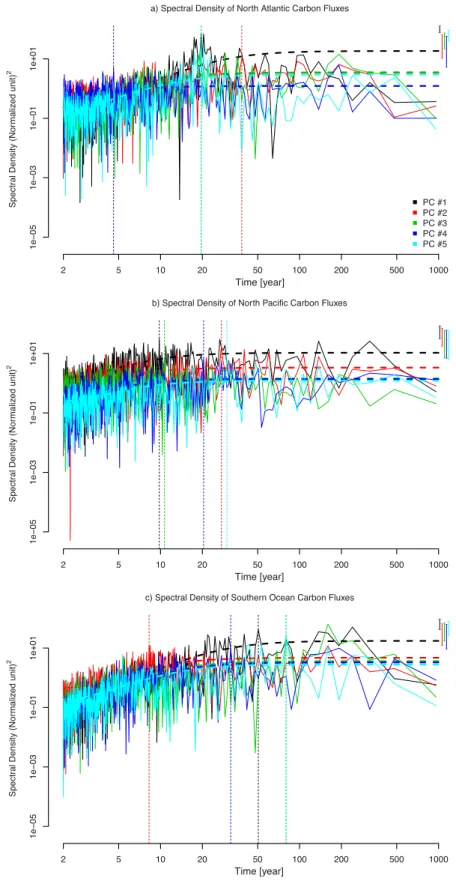
Fig. 4.Scaled spectral density of the five leading principal components of ocean carbon fluxes for(a)the North Atlantic (10◦N–80◦N),
R. S´ef´erian et al.: Decadal variability of ocean CO2fluxes 117
SSS, SST and sea-ice cover with implications on mixed-layer depth anomalies in the sub-polar gyre and Nordic Seas.
In comparison to the North Atlantic, the various modes of variability found in the North Pacific and the Southern Ocean carbon fluxes differ at the decadal time scales. In the North Pacific, modes of variability range between 10 to 30 yr (Fig. 4b). The three leading PCs, which account for 76 % of the total variance, have a large part of their energy in a time-window of 10 to 30 yr. In this time-window, the leading PC explains 44 % of the total variance and presents modes of variability at 10 and 30 yr. The standard deviation of the leading CP×EOF associated with the multi-decadal modes of variability contribute to∼0.03 Pg C yr−1to the North Pa-cific carbon flux variability.
In the Southern Ocean, the leading PC (34 % of the total variance) sheds light on a prominent mode of variability at 50 yr, while a decadal mode of variability is found in the sec-ond PC that amounts to 28 % of the total variance (Fig. 4c). Among these different modes, variability is stronger for the first 50 yr mode than for the others. This mode has a magni-tude of about 0.05 Pg C yr−1. Figure 4c shows also a cen-tennial mode of variability that appears in all of the PCs. However, this mode of variability cannot be thoroughly stud-ied with a 1000 yr time-series. Similar results are found for regional-averaged surfacepCO2(not shown).
5 Identifying drivers of low-frequency variability of
ocean carbon fluxes
A further step is to identify drivers and examine their respec-tive role in explaining the low-frequency variability of ocean carbon fluxes described in the previous sections. To find out what drivers contribute the most to the low-frequency variability of the ocean carbon fluxes, we use the variance decomposition detailed in Eq. (1) and Table 1. With this variance decomposition, we have conducted PCA analysis to identify correspondence in patterns and time variability between the fully-driven ocean carbon fluxes (f gCO2) and fluxes driven only by Alk, DIC, S and T, named respec-tivelyf gCO2-Alk, f gCO2-DIC,f gCO2-SSS andf g CO2-SST. Figures 5 to 7 show the leading EOF for the North Atlantic, the North Pacific and the Southern Ocean carbon fluxes, while lagged correlations between the leading PC of ocean carbon fluxes and dynamical drivers, i.e., sea-surface temperature, mixed-layer depth (MLD) and sea level pres-sure (SLP) are presented in Fig. 8. These dynamical drivers have been chosen since they are proxies of climate modes of variability (i.e., the AMO, the PDO, the NAM and the SAM). AMO and PDO have been estimated from the leading EOF and PC of SST, while NAM and SAM are calculated from those of SLP. Their definition differ from their canonical def-inition, especially for the AMO and PDO indices, which are usually estimated from the 10 yr running mean of detrended SST north of the Equator over the Atlantic (Enfield et al.,
2001; Kerr, 2000) and Pacific (Mantua and Hare, 2002), re-spectively. Here, our definition of AMO and PDO indices on the basis of PCA analysis show a significant correlation (>0.42) with their canonical indice estimated from the same 1000 yr long preindustrial simulation. Yet, the computation of these indices is sensitive to the latitudinal boundaries. By computing these climate indices within 0◦–80◦N, compar-ison between our definition and their canonical definition gives higher correlations (>0.6). That is, our definition of AMO and PDO mode of variability can be understood as a good approximation of their canonical definition. Same con-clusions can be drawn with the NAM and SAM indices since correlations between our definitions and their canonical def-inition is high (R∼0.7).
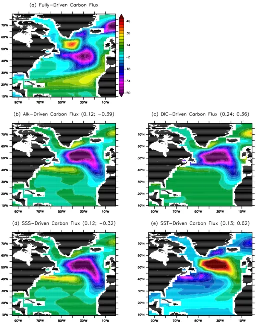
In the North Atlantic,f gCO2exhibits a horseshoe pattern, in addition to a dipole structure located close to the ocean convection sites of the Labrador and the Irminger Seas. Such features are also found in the leading EOFs off gCO2-DIC andf gCO2-SST (Fig. 5c and e). The leading EOF of the
f gCO2-SST exhibits an AMO-like pattern that is also high-lighted in Ullman et al. (2009) using the MIT OGCM reanal-ysis over 1992–2006. In our model, the leadingf gCO2-SST mode of variability displays a good match with the AMO-like pattern (Table 2). The respective correlations between PCs indicate a better match between time variability off gCO2 and that off gCO2-SST (R∼0.6) than that off gCO2-DIC (R∼0.3). Regardingf gCO2-Alk andf gCO2-SSS, the lead-ing EOF spatial patterns and the respective PCs do not dis-play correlations as strong asf gCO2-DIC andf gCO2-SST with thef gCO2(Fig. 5b and d).
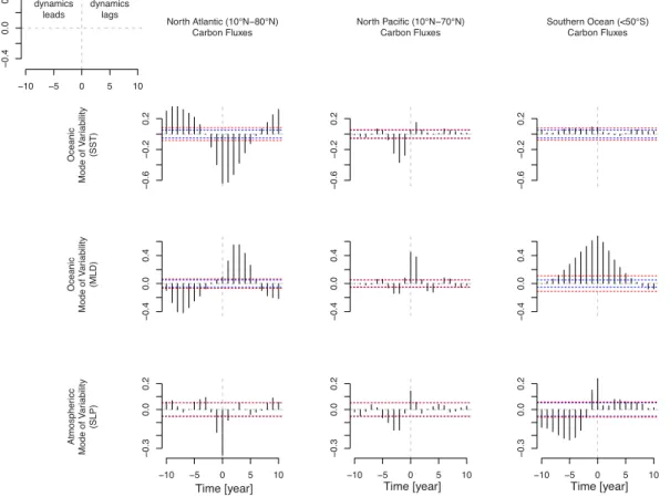
Regarding variations between SST, MLD and SLP with those off gCO2, lagged correlations indicate that the leading mode off gCO2variability is strongly in phase with that of SST (Fig. 8). Significant correlations are also found between the leading PC of SLP and that of f gCO2, but can be un-derstood as a feedback of the dynamical coupling occurring between the atmosphere and the ocean in the North Atlantic sector. Indeed, recent studies based on model simulations (Gastineau and Frankignoul, 2012) or observation-derived climate indices (Rossi et al., 2011; D’Aleo and Easterbrook, 2011; McCarthy et al., 2012) have argued that oceanic influ-ence through SST variations lead the Northern Hemisphere climate (e.g., SLP) by a few years explaining the slightly lagged inverse relationship found between the NAM/NAO and the AMO climate indices. This seems to be the case in our model since cross-correlation between the leading PC of SLP and that of SST (not shown) displays strong correlation at lag−1/0 of about 0.64. Correlation between the leading PCs off gCO2and MLD seems to indicate thatf gCO2 vari-ations lead those of MLD. Such a result may be explained by the large regional boundaries that include several sites of deep convection that are either in phase or out of phase. Nonetheless, the presence of 10-yr-lagged oscillations in cor-relation coefficients between MLD andf gCO2(also in SST)
Fig. 5.Spatial pattern of the leading empirical orthogonal function (EOF, in normalised unit) of(a)the fully-driven carbon fluxes, and that of the Alk-driven(b), DIC-driven(c), SSS-driven(d)and SST-driven(e)ocean carbon fluxes in the North Atlantic. Spatial correlations (based on EOFs) and temporal correlations (based on CPs) between the fully-driven ocean carbon fluxes and each driver-related carbon fluxes are mentioned in brackets.
can be explained by the 20 yr cycle occurring in the North Atlantic sector in this model (Escudier et al., 2013).
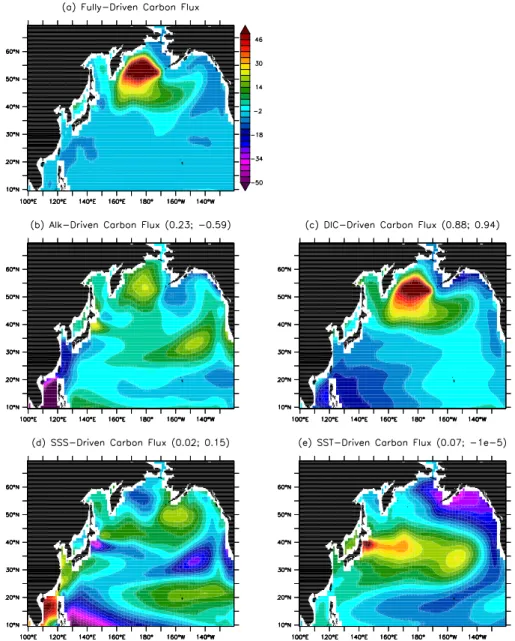
In the North Pacific, the leading EOF presents a strong positive pattern in the northern part of the domain (Fig. 6a), which is located at the same place as the strong North Pa-cific carbon outgasing (Fig. 1a). Such a pattern appears forf gCO2-DIC, but not for f gCO2-Alk,f gCO2-SSS and
f gCO2-SST (Fig. 6). The leading EOF of thef gCO2-SST exhibits a PDO-like pattern and presents good agreement with the PDO diagnosed from the leading SST EOF (Ta-ble 2). This implies that PDO imprint a low-frequency signa-ture on the ocean carbon fluxes (Valsala et al., 2012), which is
perturbed by the contribution of the other drivers to the vari-ability of the North Pacific carbon flux. The temporal correla-tions of the respective driver-related PCs with that off gCO2 demonstrate that variability driven by DIC mainly controls this mode of variability (R >0.9).
Lagged correlations (Fig. 8) between leading PCs of
R. S´ef´erian et al.: Decadal variability of ocean CO2fluxes 119
Fig. 6.Spatial pattern of the leading empirical orthogonal function (EOF, in normalised unit) of(a)the fully-driven carbon fluxes, and that of the Alk-driven(b), DIC-driven(c), SSS-driven(d)and SST-driven(e)ocean carbon fluxes in the North Pacific. Spatial correlations (based on EOFs) and temporal correlations (based on CPs) between each driver-related and the fully-driven ocean carbon fluxes are mentioned in brackets.
and SLP leading PCs are related to the mid-latitudes wind regimes over the North Pacific and can be, at worst, consid-ered as an artifact of the large regional boundaries we have chosen to define the North Pacific (10◦N–70◦N). They do not appear if one focuses above 40◦N, while the strong cor-relation betweenf gCO2and MLD and SLP are reinforced (R >0.5 at lag 0).
The Southern Ocean differs from other oceanic regions due to its zonal structure and its ocean dynamical features like the Antarctic Circumpolar Current, the westerlies forc-ings and the near-shelf dense water mass formation. Such dynamical features influence the ocean carbon cycle and are
mirrored on the leading EOF (Fig. 7a). A linear decompo-sition of drivers shows that leading EOFs of the different driver-relatedf gCO2present a good agreement with that of
f gCO2(R≥0.3). This strong spatial correlation is mainly associated with the strong spot of variability close to the Antarctic shelf. Yet, the temporal variability of thef g CO2-DIC strongly agrees with that off gCO2(R >0.9) compared to the variability of the other driver-related carbon fluxes (Fig. 7a).
To better understand Southern Ocean modes of variability, we have considered two sub-regions: one close to the Antarc-tic shelf and the sea-ice border (<65◦S) and the second that
Fig. 7.Spatial pattern of the leading empirical orthogonal function (EOF, in normalised unit) of(a)the fully-driven carbon fluxes, and that of the Alk-driven(b), DIC-driven(c), SSS-driven(d)and SST-driven(e)ocean carbon fluxes in the Southern ocean. Spatial correlations (based on EOFs) and temporal correlations (based on CPs) between the fully-driven ocean carbon fluxes and each driver-related carbon fluxes are mentioned in brackets.
extends from 65◦S to 45◦S, strongly influenced by the west-erlies. In the wind-driven region, the leading EOF off g CO2-DIC strongly matches with thef gCO2one (R∼0.8). This result agrees with several studies, which have demonstrated that westerlies influence the vertical supply of DIC through the outcrop of deep water masses (Lenton and Matear, 2007; Lovenduski et al., 2008). In this sub-region, the prominent mode of variability is at 10 yr, and appears consistently within the second mode of variability of Southern Ocean car-bon fluxes (Fig. 4c).
In the sea-ice driven region, PCA analysis shows instead thatf gCO2appears to be driven rather by SSS than by DIC
with a spatial correlation of about 0.7 and 0.5, respectively. Yet, temporal correlations indicate a better correspondence with DIC-driven variability (R∼0.87) than the SSS-driven variability (R∼0.2).
R. S´ef´erian et al.: Decadal variability of ocean CO2fluxes 121
North Atlantic (10°N−80°N) Carbon Fluxes
North Pacific (10°N−70°N) Carbon Fluxes
Southern Ocean (<50°S) Carbon Fluxes
Oceanic
Mode of V
ar
iability
(SST)
−0.6
−0.2
0.2
−0.6
−0.2
0.2
−0.6
−0.2
0.2
Oceanic
Mode of V
a
riability
(MLD)
−0.4
0.0
0
.4
−0.4
0.0
0
.4
−0.4
0.0
0
.4
Atmospher
icc
Mode of V
ar
iability
(SLP)
−0.3
0.0
0
.2
−10 −5 0 5 10
−0.3
0.0
0
.2
−10 −5 0 5 10
−0.3
0.0
0
.2
−10 −5 0 5 10
Time [year] Time [year] Time [year]
−0.4
0.0
0
.4
−10 −5 0 5 10
dynamics leads
dynamics lags
Fig. 8.Lagged correlation of leading principal components of ocean carbon fluxes and sea-surface temperature (SST), mixed-layer depth (MLD) and sea-level pressure (SLP) in the North Atlantic, the North Pacific and the Southern Ocean. Null hypothesis assessed with attest at 95 % of significance are mentioned with dashed blue lines and red lines (following Bretherton et al., 1999).
Table 2.Temporal correlation (R2) at lag 0 between the Atlantic Multidecadal Oscillation (AMO), the Pacific Decadal Oscillation (PDO), the Northern Annular Mode (NAM) and the Southern An-nular Mode (SAM) with the regionally integrated carbon fluxes re-lated to each drivers (i.e., Alk-f gCO2, DIC-f gCO2, SSS-f gCO2,
SST-f gCO2). Correlations between dynamical indices and
region-ally integrated carbon fluxes are done in the same region and are assessed withttest at 95 % of significance are mentioned in bold (following Bretherton et al., 1999). AMO and PDO indices have been estimated from the leading PC of SST over the North Atlantic (10◦N–80◦N) and the North Pacific (10◦N–70◦N), respectively. NAM and SAM indices have been computed from the leading PC of SLP over the North Atlantic (10◦N–80◦N) and the Southern ocean(<50◦S), respectively.
Alk-f gCO2 DIC-f gCO2 SSS-f gCO2 SST-f gCO2
AMO 0.79 0.68 0.77 0.95
PDO 0.42 0.004 0.73 0.95
NAM 0.05 0.01 0.02 0.17
SAM 0.13 0.30 0.19 0.59
the wind forcing influences the subduction of intermediate and mode waters around Antarctica (Sall´ee et al., 2012) and Ekman-induced upwelling of deep-core waters. At decadal time scales, it is likely that the SAM oscillations could influ-ence the Deacon cell through the Ekman-induced transport bringing in turn DIC-rich deep waters (Table 2). This may explain why we find a lag at 5–8 yr for the cross-correlation between SLP andf gCO2leading PCs. In the whole Southern Ocean region (<50◦S), this mode linking SAM and ocean carbon fluxes, appears only as a second mode with a cor-relation of 0.7 at lag 0 indicating that this mechanism is of second order compared to the deep-mixing events linked to ocean-sea ice interactions.
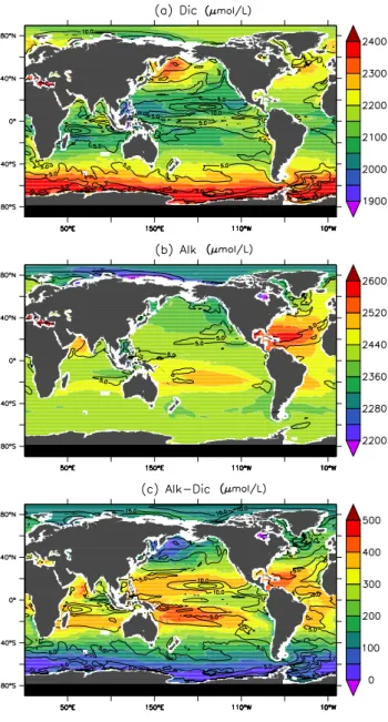
In order to show how variability in ocean dynamics can interact with water mass properties in terms of dissolved car-bon, we show the long-term mean concentrations and asso-ciated standard deviations of DIC, Alk and Alk-DIC at the maximum (winter) of the mixed-layer depth (Fig. 9). Alk-DIC serves as a good approximation for the carbonate ion concentration (Sarmiento and Gruber, 2006). This is a proxy for the buffer capacity of seawater and, hence, the chemi-cal capacity for the ocean to take up atmospheric CO2. Fig-ure 9c indicates that the sub-surface water masses are rich in
Fig. 9.Long-term mean of(a)DIC,(b)Alk and(c)Alk-DIC con-centrations (in µmol L−1) at maximum (winter) mixed-layer depth. Variability represented by the standard deviation of the concentra-tions of(a)DIC,(b)Alk and(c)Alk-DIC is contoured.
DIC content with an Alk-DIC concentration close to 0. It ap-pears thus clearly that, of the three different oceanic regions, the chemical properties of the North Pacific and the Southern Ocean sub-surface water masses differ greatly from those of the North Atlantic.
In regions of water mass formation (i.e., North Atlantic), the water mass content in DIC is set by air-sea interaction and biology and is, hence, sensitive to both variations in at-mospheric forcings and variations in surface ocean proper-ties (i.e., SST). In regions of water mass outcrops and trans-formations (i.e., North Pacific and Southern Ocean), water mass content in DIC is instead enriched by remineralisation
processes occurring below the surface. Consequently, re-sponse of ocean carbon fluxes driven at first order by the dif-ference in partial pressure of CO2 between the atmosphere and the surface waters (which have been replenished in DIC due to DIC-rich deep water mass upwelling) overcomes the variability inherited from ocean thermodynamical variables like the SST and SSS. Such processes are highlighted in Fig. 10 showing, respectively, long-term mean state and vari-ance profile of pCO2, Alk-pCO2, DIC-pCO2, SSS-pCO2 and SST-pCO2. Long-term mean vertical profiles ofpCO2 exhibits large differences compared to pCO2-Alk, p CO2-DIC,pCO2-SSS andpCO2-SST at 500 m between the North Atlantic, the North Pacific and the Southern Ocean (Fig. 10a– c). ThepCO2 long-term mean profile in the North Atlantic displays an important vertical gradient in the first 100 m and a well-mixed profile below (Fig. 10a). This is not the case for the North Pacific and the Southern Ocean pCO2 pro-files, which exhibit strong gradients from surface to 500 m (Fig. 10b and c). Within these two regions, the variability of
pCO2at 500 m (here the standard deviation) is 5- to 6-fold stronger than the North Atlantic one.
Figure 10j–l present results of a multiple linear regression on the basis of Eq. (1). The statistical t test on a parame-ter slope (here Alk, DIC,SandT) can be considered as an attribution test. That is, there is attribution of the variabil-ity driven by a given parameter to the pCO2 variability if the slope is close to 1. There is no attribution if the slope is negative or if its confidence interval at 95 % (given by ver-tical lines on Fig. 10j–l) on of the slope includes 0. Conse-quently, our attribution test demonstrates that the variations (Fig. 10d–f) ofpCO2at depth are mostly explained by varia-tions in temperature in the North Atlantic with an attribution factor close to 1, while North Pacific and Southern Ocean
pCO2 variations at depth are set by variations in DIC with an attribution factor close to 1. Others variables likeS and Alk have a poor contribution to thepCO2variability.
6 Conclusions
R. S´ef´erian et al.: Decadal variability of ocean CO2fluxes 123
Mean (ppm)
Depth (m)
260 280 300 320
500
400
300
200
100
a) North Atlantic pCO2 long−term mean
Mean (ppm)
300 400 500 600
500
400
300
200
100
b) North Pacific pCO2 long−term mean
pCO2 pCO2−DIC pCO2−ALK pCO2−T pCO2−S
Mean (ppm)
350 450 550
500
400
300
200
100
c) Southern Ocean pCO2 long−term mean
Standard Deviation (ppm)
Depth (m)
0 5 10 15 20
500
400
300
200
100
d) North Atlantic pCO2 variability
pCO2 pCO2−DIC pCO2−ALK pCO2−T pCO2−S
Standard Deviation (ppm)
0 5 10 15 20 25
500
400
300
200
100
e) North Pacific pCO2 variability
Standard Deviation (ppm)
0 10 20 30 40
500
400
300
200
100
f) Southern Ocean pCO2 variability
Standard Deviation (unit)
Depth (m)
0 0.2 0.5 0.7 0.9
0 11.5 23 34.5 46
500
400
300
200
100
g) North Atlantic drivers variability
Standard Deviation (unit)
0 0.2 0.3 0.5 0.7
0 8.4 16.9 25.3 33.8
500
400
300
200
100
h) North Pacific drivers variability
DIC ALK T S
Standard Deviation (unit)
0 0.1 0.2 0.2 0.3
0 3.8 7.6 11.4 15.2
500
400
300
200
100
i) Southern Ocean drivers variability
Drivers
Attr
ib
ution F
a
ctors
_ _
_ _
_
_
−4
0
2
4
Alk DIC S T j) North Atlantic drivers Attribution
Drivers
_ _
_ _
−4
0
2
4
Alk DIC S T l) Southern Ocean drivers Attribution
Drivers _
_ _
_ _
−4
0
2
4
Alk DIC S T k) North Pacific drivers Attribution
Fig. 10.Scaled spectral density of the five leading principal components of ocean carbon fluxes for(a)the North Atlantic (10◦N–80◦N),
(b)the North Pacific (10◦N–70◦N) and(c)the Southern ocean(<50◦S). Dashed lines represent fitted AR1 theoretical spectrum according to the Yule-Walker estimation, while the linear dashed lines indicate the maximum of spectral density for each principal component. Confidence intervals at 95 % of significance of the scaled spectral density maximum are indicated by vertical bars; they have been computed from a (scaled)χ2distribution.
in the North Pacific and in the Southern Ocean are mostly driven by the variability of the dissolved inorganic carbon of surface waters. The latter is controlled by the vertical supply of dissolved inorganic carbon of subsurface waters, through the dynamical influence of wind forcings or deep-mixing
events, which controls the shape and the timing of the carbon flux variability within these regions. In the North Atlantic, the ocean carbon flux is primarily driven by the variability of sea surface temperature. This contrast in dynamical and bio-geochemical drivers of ocean carbon flux variations between
the three oceanic regions is set in part by the large-scale cir-culation of water masses and their biogeochemical proper-ties. That is, in regions of dense water mass outcrops and transformations, variations in vertical supply of dissolved in-organic carbon (owing to Ekman-induced upwelling or deep-mixing events) are of larger amplitude than the variations in-herited from thermodynamical properties of surface waters (owing to ocean-atmosphere or ocean-sea ice interactions). This is not the case in regions of dense water mass formation. The fact that low-frequency variations in ocean carbon fluxes are simulated in our model within high latitude oceans is consistent with previous studies conducted on dynamical fields like sea surface temperature, surface air temperature or precipitation (e.g. Boer, 2004, 2000). Of particular interest, a similar study with the same model (i.e., IPSL-CM5A-LR) by Persechino et al. (2013) demonstrates that decadal variations of sea surface temperature amount for 20 % (with a maxi-mum of 50 %) of their interannual variations within the North Atlantic sector. Comparatively, ocean carbon fluxes exhibit low-frequency variations much stronger (∼20–40 %) than those of sea surface temperature. Such differences between low-frequency variations of ocean carbon fluxes and other dynamical fields are even stronger in the Southern Ocean, where Boer (2004) shows that multi-model zonal average variations of surface air temperature at decadal time scales only accounts for 10 % of the interannual variability. In our case, decadal variations of ocean carbon fluxes within Sub-polar and Polar Regions of the Antarctic sector amounts to up to 25 %. Such features can be explained by the statistical properties of ocean carbon fluxes, which cannot be approx-imated with a first-order autoregressive process (like other dynamical variables mentioned above) indicating that long-term memory processes likely drive ocean carbon fluxes (and potentially other biogeochemical fluxes like the carbon ex-port, the primary productivity and the remineralisation).
Also related to long-memory processes, all of these oceanic regions exhibit multi-centennial modes of variability (>150 yr) that cannot be assessed with a 1000 yr preindus-trial simulation. Similar multi-centennial modes of variabil-ity have also been revealed in surface temperature, sea-surface salinity, sea-ice volume and Atlantic meridional over-turning for the GFDL-CM2.1 climate model (Delworth and Zeng, 2012). Interestingly, this study has hypothesised that these modes are controlled by interactions between ocean and sea-ice dynamics. It is, thus, likely that such interactions could impact air-sea carbon fluxes.
At decadal time scales, processes related to these low-frequency modes of variability agree with process-based studies (Ullman et al., 2009; Corbi`ere et al., 2007; L¨optien and Eden, 2010; Thomas et al., 2008; Metzl et al., 2010; Lovenduski et al., 2008; Takahashi et al., 2006), which sug-gest that variations in air-sea fluxes (or sea-water partial pres-sure) of carbon are driven either by the sea surface tempera-ture or by the vertical supply of dissolved inorganic carbon. However, our results seem to indicate that vertical supply of
dissolved organic carbon related to the atmospheric modes of variability are of major importance in the North Pacific and the Southern Ocean, and not directly in the North Atlantic. Indeed, in our model, atmospheric modes of variability like the North Atlantic Oscillation weakly impact the ocean car-bon fluxes (or very locally) as mentioned in Keller et al. (2012), while they can be projected on ocean-atmosphere coupled modes like the Atlantic Multi-decadal Oscillation. Nevertheless, we shall keep in mind that these findings are subject to criticism because they are related to the fact that we use only one Earth System Model. Consequently, we can wonder: (1) how do modes of variability of different Earth System Models compare to each other? (2) Is there any con-sistency between their drivers? Therefore, studies like the one conducted by Keller et al. (2012) are of great interest in order to understand how a given Earth System Model be-haves in a multi-model perspective.
Yet, even in a multi-model perspective such as CMIP5, one of the major uncertainties in the quantification of the internal variability of ocean carbon fluxes (as others variables) would be related to the horizontal resolution of the considered ocean model (>1◦ in most of the CMIP5 models). Recent litera-ture (e.g. Penduff et al., 2010, 2011; Lovenduski et al., 2013) highlights that meso-scale activity in eddying-regions like the Southern Ocean strongly enhances interannual variability of ocean variables – such as ocean turbulence. The impact of meso-scale activity could likely amplify the interannual vari-ability of the ocean carbon fluxes. Since the varivari-ability of the ocean carbon fluxes is influenced by the long-term mean state of ocean carbon-related fields, this variability could be affected by the response of westerlies-induced transport to the model resolution (e.g. Farneti et al., 2010; Hofmann and Morales Maqueda, 2011) and, hence, model biases (Swart and Fyfe, 2011).
Notwithstanding the limitations of the model, our find-ings provide a first step to better understand the role of the internal variability (as a part of the natural variability) ver-sus that of the anthropogenic forced variability on the ocean carbon fluxes. Our results demonstrate that care should be taken while analysing short-term changes with delta or bi-ases correction methods, which consist in applying model anomaly to observed fields (e.g. Sarmiento et al., 1992). Indeed, these methods generally assume that the long-term mean state does not affect the variability, while our results demonstrate that it does matter in some oceanic regions like the Southern Ocean and the North Pacific. This is not the case for long-term changes for which rising atmospheric CO2and climate change can impact ocean carbon fluxes much more strongly than their decadal variations (Matear and Lenton, 2008; Lenton and Matear, 2007; S´ef´erian et al., 2012; Roy et al., 2011).
R. S´ef´erian et al.: Decadal variability of ocean CO2fluxes 125
anthropogenic trend (McKinley et al., 2011). Both issues are important, but the observational needs are different. It seems that the observational needs are larger in oceanic regions where low frequency modes of variability take place than in those dominated by interannual variability. Yet, relevant spatiotemporal scales are unknown to ensure an optimal and efficient sampling strategy. To assess and quantify the obser-vational need in the view of studying the natural variability of ocean carbon fluxes, similar studies to this of Lenton et al. (2009) could be a possible alternative.
Acknowledgements. We sincerely thank Marina Levy, Corinne Le
Qu´er´e, Marion Gehlen, Mehera Kidston and the two anonymous reviewers for their useful comments on that paper. This work was supported by GENCI (Grand Equipement National de Calcul Intensif) at CCRT (Centre de Calcul Recherche et Technologie), allocation 016178 and through EU FP7 project CARBOCHANGE “Changes in carbon uptake and emissions by oceans in a changing climate” which received funding from the European Community’s Seventh Framework Programme under grant agreement no. 264879.
Edited by: C. Heinze
References
Aumont, O. and Bopp, L.: Globalizing results from ocean in situ iron fertilization studies, Global Biogeochem. Cy., 20, GB2017, doi:10.1029/2005GB002591, 2006.
Aumont, O., Maier-Reimer, E., Blain, S., and Monfray, P.: An ecosystem model of the global ocean including Fe, Si, P colimitations, Global Biogeochem. Cy., 17, 1060, doi:10.1029/2001GB001745, 2003.
Bakker, D. C. E., Pfeil, B., Olsen, A., Sabine, C. L., Metzl, N., Han-kin, S., Koyuk, H., Kozyr, A., Malczyk, J., Manke, A., and Tel-szewski, M.: Global data products help assess changes to ocean carbon sink, Eos Trans. AGU, 93, doi:10.1029/2012EO120001, 2012.
Bates, N. R.: Interannual variability of the oceanic CO2 sink in the subtropical gyre of the North Atlantic Ocean over the last 2 decades, J. Geophys. Res., 112, C09013, doi:10.1029/2006JC003759, 2007.
Bates, N. R.: Multi-decadal uptake of carbon dioxide into subtropi-cal mode water of the North Atlantic Ocean, Biogeosciences, 9, 2649–2659, doi:10.5194/bg-9-2649-2012, 2012.
Bates, N. R., Best, M. H. P., Neely, K., Garley, R., Dickson, A. G., and Johnson, R. J.: Detecting anthropogenic carbon dioxide uptake and ocean acidification in the North Atlantic Ocean, Bio-geosciences, 9, 2509–2522, doi:10.5194/bg-9-2509-2012, 2012. Boening, C. W., Dispert, A., Visbeck, M., Rintoul, S., and Schwarzkopf, F. U.: The response of the Antarctic Circumpo-lar Current to recent climate change, Nat. Geosci., 1, 864–869, 2008.
Boer, G. J.: A study of atmosphere-ocean
predictabil-ity on long time scales, Clim. Dynam., 16, 469–477, doi:10.1007/s003820050340, 2000.
Boer, G. J.: Long time-scale potential predictability in an en-semble of coupled climate models, Clim. Dynam., 23, 29–44, doi:10.1007/s00382-004-0419-8, 2004.
Boer, G. J. and Lambert, S. J.: Multi-model decadal potential pre-dictability of precipitation and temperature, Geophys. Res. Lett., 35, L05706, doi:10.1029/2008GL033234, 2008.
Bretherton, C. S., Widmann, M., Dymnikov, V. P., Wallace, J. M., and Blad´e, I.: The effective number of spatial degrees of freedom of a time-varying field, J. Climate, 12, 1990–2009, 1999. Brown, P. J., Bakker, D. C. E., Schuster, U., and
Wat-son, A. J.: Anthropogenic carbon accumulation in the sub-tropical North Atlantic, J. Geophys. Res., 115, C04016, doi:10.1029/2008JC005043, 2010.
Chavez, F. P., Strutton, P. G., Friederich, G. E., Feely, R., Feldman, G. C., Foley, D. G., and McPhaden, M. J.: Bi-ological and Chemical Response of the Equatorial Pacific Ocean to the 1997–98 El Ni˜no, Science, 286, 2126–2131, doi:10.1126/science.286.5447.2126, 1999.
Corbi`ere, A., Metzl, N., Reverdin, G., Brunet, C., and Takahashi, T.: Interannual and decadal variability of the oceanic carbon sink in the North Atlantic subpolar gyre, Tellus B, 59, 168–178, doi:10.1111/j.1600-0889.2006.00232.x, 2007.
D’Aleo, J. and Easterbrook, D.: Chapter 5 – Relationship of Mul-tidecadal Global Temperatures to MulMul-tidecadal Oceanic Oscil-lations, in: Evidence-Based Climate Science, Elsevier, Boston, 161–184, doi:10.1016/B978-0-12-385956-3.10005-1, 2011. Delworth, T. L. and Zeng, F.: Multicentennial variability
of the Atlantic meridional overturning circulation and its climatic influence in a 4000 year simulation of the GFDL CM2.1 climate model, Geophys. Res. Lett., 39, L13702, doi:10.1029/2012GL052107, 2012.
Doney, S. C., Lindsay, K., Fung, I., and John, J.: Natural Variabil-ity in a Stable, 1000-Yr Global Coupled Climate–Carbon Cycle Simulation, J. Climate, 19, 3033–3054, doi:10.1175/JCLI3783.1, 2006.
Dufresne, J.-L., Foujouls, M.-A., Denvil, S., Caubel, A., Marti, O., Aumont, O., Balkansky, Y., Bekki, S., Bellenger, S., Benshila, R., Bony, S., Bopp, L., Braconnot, P., and Brockmann, P.: The IPSL-CM5A Earth System Model: general description and cli-mate change projections, Clim. Dynam., in press, 2013. Enfield, D. B., Mestas Nu˜nez, A. M., and Trimble, P. J.: The
At-lantic Multidecadal Oscillation and its relation to rainfall and river flows in the continental U.S., Geophys. Res. Lett., 28, 2077–2080, doi:10.1029/2000GL012745, 2001.
Escudier, R., Mignot, J., and Swingedouw, D.: A 20-year coupled ocean-sea ice-atmosphere variability mode in the North Atlantic in an AOGCM, Clim. Dynam., doi:10.1007/s00382-012-1402-4, in press, 2013.
Farneti, R., Delworth, T. L., Rosati, A. J., Griffies, S. M., and Zeng, F.: The Role of Mesoscale Eddies in the Rectification of the Southern Ocean Response to Climate Change, J. Phys. Oceanogr., 40, 1539–1557, doi:10.1175/2010JPO4353.1, 2010. Fichefet, T. and Maqueda, M. A. M.: Sensitivity of a global sea ice
model to the treatment of ice thermodynamics and dynamics, J. Geophys. Res., 102, 12609–12646, 1997.
Frankignoul, C.: Sea surface temperature anomalies, planetary waves, and air-sea feedback in the middle latitudes, Rev. Geo-phys., 23, 357–390, doi:10.1029/RG023i004p00357, 1985.
Gastineau, G. and Frankignoul, C.: Cold-season atmospheric response to the natural variability of the Atlantic merid-ional overturning circulation, Clim. Dynam., 39, 37–57, doi:10.1007/s00382-011-1109-y, 2012.
Gruber, N., Keeling, C., and Bates, N.: Interannual variability in the North Atlantic Ocean carbon sink, Science, 298, 2374–2378, 2002.
Gurney, K. R., Law, R. M., Denning, A. S., Rayner, P. J., Baker, D., Bousquet, P., Bruhwiler, L., Chen, Y.-H., Ciais, P., Fan, S., Fung, I. Y., Gloor, M., Heimann, M., Higuchi, K., John, J., Maki, T., Maksyutov, S., Masarie, K., Peylin, P., Prather, M., Pak, B. C., Randerson, J., Sarmiento, J., Taguchi, S., Takahashi, T., and Yuen, C.-W.: Towards robust regional estimates of CO2sources
and sinks using atmospheric transport models, Nature, 415, 626– 630, doi:10.1038/415626a, 2002.
Hofmann, M. and Morales Maqueda, M. A.: The response of South-ern Ocean eddies to increased midlatitude westerlies: A non-eddy resolving model study, Geophys. Res. Lett., 38, L03605, doi:10.1029/2010GL045972, 2011.
Hourdin, F., Foujols, M.-A., Codron, F., Guemas, V., Dufresne, J.-L., Bony, S., Denvil, S., Guez, L., Lott, F., Ghattas, J., Bra-connot, P., Marti, O., Meurdesoif, Y., and Bopp, L.: Impact of the LMDZ atmospheric grid configuration on the climate and sensitivity of the IPSL-CM5A coupled model, Clim. Dynam., doi:10.1007/s00382-012-1411-3, in press, 2013.
Keller, K. M., Joos, F., Raible,, C. C., Cocco, V., Froelicher, T. L., Dunne, J. P., Gehlen, M., Roy, T., Bopp, L., Orr, J. C., Tjipu-tra, J., Heinze, C., Segschneider, J., and Metzl, N.: Variability of the Ocean Carbon Cycle in Response to the North Atlantic Os-cillation, Tellus B, 64, 18738, doi:10.3402/tellusb.v64i0.18738, 2012.
Kerr, R. A.: A North Atlantic Climate Pacemaker for the Centuries, Science, 288, 1984–1985, 2000.
Krinner, G., Viovy, N., de Noblet-Ducoudr´e, N., Og´ee, J., Polcher, J., Friedlingstein, P., Ciais, P., Sitch, S., and Prentice, I.: A dynamic global vegetation model for studies of the coupled atmosphere-biosphere system, Global Biogeochem. Cy., 19, 1– 33, 2005.
Latif, M., Collins, M., Pohlmann, H., and Keenlyside, N.: A review of predictability studies of Atlantic sector climate on decadal time scales, J. Climate, 19, 5971–5987, doi:10.1175/JCLI3945.1, 2006.
Lenton, A. and Matear, R. J.: Role of the Southern Annular Mode (SAM) in Southern Ocean CO2uptake, Global Biogeochem. Cy., 21, GB2016, doi:10.1029/2006GB002714, 2007.
Lenton, A., Bopp, L., and Matear, R. J.: Strategies for high-latitude northern hemisphere CO2sampling now and in the future,
Deep-Sea Res. Pt. II, 56, 523–532, doi:10.1016/j.dsr2.2008.12.008, 2009.
Le Qu´er´e, C., Roedenbeck, C., Buitenhuis, E. T., Conway, T. J., Langenfelds, R., Gomez, A., Labuschagne, C., Ramonet, M., Nakazawa, T., Metzl, N., Gillett, N., and Heimann, M.: Satu-ration of the Southern Ocean CO2 sink due to recent climate
change, Science, 316, 1735–1738, doi:10.1126/science.1136188, 2007.
L¨optien, U. and Eden, C.: Multidecadal CO2 uptake
variabil-ity of the North Atlantic, J. Geophys. Res., 115, D12113, doi:10.1029/2009JD012431, 2010.
Lovenduski, N. S. and Ito, T.: The future evolution of the
Southern Ocean CO2 sink, J. Mar. Res., 67, 597–617,
doi:10.1357/002224009791218832, 2009.
Lovenduski, N. S., Gruber, N., and Doney, S. C.: Toward a mechanistic understanding of the decadal trends in the South-ern Ocean carbon sink, Global Biogeochem. Cy., 22, GB3016, doi:10.1029/2007GB003139, 2008.
Lovenduski, N. S., Long, M. C., Gent, P. R., and Lindsay, K.: Multi-decadal trends in the advection and mixing of natural car-bon in the Southern Ocean, Geophys. Res. Lett., 40, 139–142, doi:10.1029/2012GL054483, 2013.
Madec, G.: NEMO ocean engine, France Edn., Institut Pierre-Simon Laplace (IPSL), institut pierre-simon laplace (ipsl), France, 2008.
Mantua, N. and Hare, S.: The Pacific Decadal Oscillation, J. Oceanogr., 58, 35–44, doi:10.1023/A:1015820616384, 2002. Marti, O., Braconnot, P., Dufresne, J.-L., Bellier, J., Benshila, R.,
Bony, S., Brockmann, P., Cadule, P., Caubel, A., Codron, F., No-blet, N., Denvil, S., Fairhead, L., Fichefet, T., Foujols, M. A., Friedlingstein, P., Goosse, H., Grandpeix, J. Y., Guilyardi, E., Hourdin, F., Idelkadi, A., Kageyama, M., Krinner, G., L´evy, C., Madec, G., Mignot, J., Musat, I., Swingedouw, D., and Talandier, C.: Key features of the IPSL ocean atmosphere model and its sensitivity to atmospheric resolution, Clim. Dynam., 34, 1–26, doi:10.1007/s00382-009-0640-6, 2009.
Matear, R. J. and Lenton, A.: Impact of Historical Climate Change on the Southern Ocean Carbon Cycle, J. Climate, 21, 5820–5834, doi:10.1175/2008JCLI2194.1, 2008.
Mauget, S. A., Cordero, E. C., and Brown, P. T.: Evaluating Mod-eled Intra- to Multi-decadal Climate Variability Using Running Mann-Whitney Z Statistics, J. Climate, 25, 110824105314003, doi:10.1175/JCLI-D-11-00211.1, 2011.
McCarthy, G. D., King, B. A., Cipollini, P., MCDonagh, E., Blun-dell, J. R., and Biastoch, A.: On the sub-decadal variability of South Atlantic Antarctic Intermediate Water, Geophys. Res. Lett., 39, L10605, doi:10.1029/2012GL051270, 2012.
McKinley, G. A., Follows, M. J., and Marshall, J.: Mechanisms of air-sea CO2 flux variability in the equatorial Pacific and
the North Atlantic, Global Biogeochem. Cy., 18, GB2011, doi:10.1029/2003GB002179, 2004.
McKinley, G. A., Fay, A. R., Takahashi, T., and Metzl, N.: Convergence of atmospheric and North Atlantic carbon diox-ide trends on multdiox-idecadal timescales, Nat. Geosci., 4, 1–5, doi:10.1038/ngeo1193, 2011.
Metzl, N., Corbi`ere, A., Reverdin, G., Lenton, A., Takahashi, T., Olsen, A., Johannessen, T., Pierrot, D., Wanninkhof, R., ´Olafsd´ottir, S. R., Olafsson, J., and Ramonet, M.: Re-cent acceleration of the sea surface f gCO2 growth rate in
the North Atlantic subpolar gyre (1993–2008) revealed by winter observations, Global Biogeochem. Cy., 24, GB4004, doi:10.1029/2009GB003658, 2010.
Mikaloff Fletcher, S. E., Gruber, N., Jacobson, A. R., Gloor, M., Doney, S. C., Dutkiewicz, S., Gerber, M., Follows, M., Joos, F., Lindsay, K., Menemenlis, D., Mouchet, A., M¨uller, S. A., and Sarmiento, J. L.: Inverse estimates of the oceanic sources and sinks of natural CO2 and the implied
R. S´ef´erian et al.: Decadal variability of ocean CO2fluxes 127
Penduff, T., Juza, M., Brodeau, L., Smith, G. C., Barnier, B., Mo-lines, J.-M., Treguier, A.-M., and Madec, G.: Impact of global ocean model resolution on sea-level variability with emphasis on interannual time scales, Ocean Sci., 6, 269–284, doi:10.5194/os-6-269-2010, 2010.
Penduff, T., Juza, M., Barnier, B., Zika, J., Dewar, W. K., Treguier, A.-M., Molines, J.-M., and Audiffren, N.: Sea Level Expres-sion of Intrinsic and Forced Ocean Variabilities at Interannual Time Scales, J. Climate, 24, 5652–5670, doi:10.1175/JCLI-D-11-00077.1, 2011.
Persechino, A., Mignot, J., Swingedouw, D., Labetoulle, S., and Guilyardi, E.: Decadal predictability of the Atlantic merid-ional overturning circulation and climate in the IPSL-CM5A-LR model, Clim. Dynam., doi:10.1007/s00382-012-1466-1, in press, 2013.
Rossi, A., Massei, N., and Laignel, B.: A synthesis of the time-scale variability of commonly used climate indices using con-tinuous wavelet transform, Global Planet. Change, 78, 1–13, doi:10.1016/j.gloplacha.2011.04.008, 2011.
Roy, T., Bopp, L., Gehlen, M., Schneider, B., Cadule, P., Fr¨olicher, T. L., Segschneider, J., Tjiputra, J., Heinze, C., and Joos, F.: Regional Impacts of Climate Change and At-mospheric CO2 on Future Ocean Carbon Uptake: A
Multi-model Linear Feedback Analysis, J. Climate, 24, 2300–2318, doi:10.1175/2010JCLI3787.1, 2011.
Sall´ee, J.-B., Matear, R. J., Rintoul, S. R., and Lenton, A.: Localized subduction of anthropogenic carbon dioxide in the Southern Hemisphere oceans, Nat. Geosci., 5, 579–584, doi:10.1038/ngeo1523, 2012.
Sarmiento, J. L. and Gruber, N.: Ocean Biogeochemical Dynamics, Princeton University Press, 2006.
Sarmiento, J. L., Orr, J. C., and Siegenthaler, U.: A perturbation simulation of CO2 uptake in an ocean general circulation model, J. Geophys. Res., 97, 3621–3645, doi:10.1029/91JC02849, 1992. Schuster, U., Watson, A. J., Bates, N. R., Corbiere, A., Gonz´alez-D´avila, M., Metzl, N., Pierrot, D., and Santana-Casiano, M.: Trends in North Atlantic sea-surface f gCO2
from 1990 to 2006, Deep-Sea Res. Pt. II, 56, 620–629, doi:10.1016/j.dsr2.2008.12.011, 2009.
S´ef´erian, R., Iudicone, D., Bopp, L., Roy, T., and Madec, G.: Water Mass Analysis of Effect of Climate Change on Air-Sea CO2 Fluxes: The Southern Ocean, J. Climate, 25, 3894–3908, doi:10.1175/JCLI-D-11-00291.1, 2012.
S´ef´erian, Roland, Bopp, L., Gehlen, M., Orr, J., Eth´e, C., Cadule, P., Aumont, O., Salas y M´elia, D., Voldoire, A., and Madec, G.: Skill assessment of three earth system models with common marine biogeochemistry, Clim. Dynam., doi:10.1007/s00382-012-1362-8, in press, 2013.
Swart, N. C. and Fyfe, J. C.: Ocean carbon uptake and storage influ-enced by wind bias in global climate models, Nat. Clim. Change, 2, 47–52, doi:10.1038/nclimate1289, 2011.
Takahashi, T.: Climatological mean and decadal change in
surface ocean pCO2, and net sea-air CO2 flux over
the global oceans, Deep-Sea Res. Pt. II, 56, 554–577, doi:10.1016/j.dsr2.2008.12.009, 2009.
Takahashi, T., Olafsson, J., Goddard, J. G., Chipman, D. W., and Sutherland, S. C.: Seasonal variation of CO2and nutrients in the
high-latitude surface oceans: A comparative study, Global Bio-geochem. Cy., 7, 843–878, doi:10.1029/93GB02263, 1993. Takahashi, T., Sutherland, S. C., Sweeney, C., Poisson, A., Metzl,
N., Tilbrook, B., Bates, N., Wanninkhof, R., Feely, R. A., Sabine, C., Olafsson, J., and Nojiri, Y.: Global sea-air CO2flux based
on climatological surface oceanpCO2, and seasonal biological and temperature effects, Deep-Sea Res. Pt. II, 49, 1601–1622, doi:10.1016/S0967-0645(02)00003-6, 2002.
Takahashi, T., Sutherland, S. C., Feely, R. A., and Wanninkhof, R.: Decadal change of the surface waterpCO2in the North Pacific:
A synthesis of 35 years of observations, J. Geophys. Res., 111, C07S05, doi:10.1029/2005JC003074, 2006.
Thomas, H., Friederike Prowe, A. E., van Heuven, S., Bozec, Y., de Baar, H. J. W., Schiettecatte, L.-S., Suykens, K., Kon´e, M., Borges, A. V., Lima, I. D., and Doney, S. C.: Rapid decline of the CO2buffering capacity in the North Sea and implications for
the North Atlantic Ocean, Global Biogeochem. Cy., 21, GB4001, doi:10.1029/2006GB002825, 2007.
Thomas, H., Friederike Prowe, A. E., Lima, I. D., Doney, S. C., Wanninkhof, R., Greatbatch, R. J., Schuster, U., and Corbi`ere, A.: Changes in the North Atlantic Oscillation influence CO2
up-take in the North Atlantic over the past 2 decades, Global Bio-geochem. Cy., 22, GB4027, doi:10.1029/2007GB003167, 2008. Thompson, D. W. J. and Wallace, J. M.: Annular modes in the ex-tratropical circulation, Part I: month-to-month variability, J. Cli-mate, 13, 1000–1016, 2000.
Thompson, D. W. J., Wallace, J. M., and Hegerl, G. C.: Annular Modes in the Extratropical Circulation, Part II: Trends, J. Cli-mate, 13, 1018–1036, 2000.
Torrence, C. and Compo, G. P.: A Practical Guide to Wavelet Analysis, B. Am. Meteorol. Soc., 79, 61–78, doi:10.1175/1520-0477(1998)079<0061:APGTWA>2.0.CO;2, 1998.
Ullman, D. J., McKinley, G. A., Bennington, V., and
Dutkiewicz, S.: Trends in the North Atlantic carbon sink: 1992–2006, Global Biogeochem. Cy., 23, GB4011, doi:10.1029/2008GB003383, 2009.
Valsala, V., Maksyutov, S., Telszewski, M., Nakaoka, S., Nojiri, Y., Ikeda, M., and Murtugudde, R.: Climate impacts on the struc-tures of the North Pacific air-sea CO2flux variability,
Biogeo-sciences, 9, 477–492, doi:10.5194/bg-9-477-2012, 2012. Von Storch, H. and Zwiers, F.: Statistical Analysis in Climate
Re-search – Hans Von Storch, Francis W. Zwiers – Google Books, Cambridge University Press, 2002.
Wang, S. and Moore, J. K.: Variability of primary production and air-sea CO2flux in the Southern Ocean, Global Biogeochem.
Cy., 26, GB1008, doi:10.1029/2010GB003981, 2012.
Wanninkhof, R.: A relationship between wind speed and gas ex-change over the ocean, J. Geophys. Res., 97, 7373–7382, 1992. Watson, A. J., Metzl, N., and Schuster, U.: Monitoring and
interpret-ing the ocean uptake of atmospheric CO2, Philosophical
Trans-actions of the Royal Society A: Mathematical, Phys. Eng. Sci., 369, 1997–2008, doi:10.1098/rsta.2011.0060, 2011.
Zwiers, F.: Interannual variability and predictability in an ensemble of AMIP climate simulations conducted with the CCC GCM2, Clim. Dynam., 12, 825–847, 1996.