Design of Total Sliding-Mode Control for Chua's Chaotic Circuit

(1)

Design of Total Sliding-Mode Control for Chua’s Chaotic Circuit

Rong-Jong Wai, MEMBER,IAENG,and You-Wei Lin

Abstract−This study mainly focuses on the development of a

total sliding-mode control (TSMC) strategy for a Chua’s chaotic circuit. The TSMC scheme, which is insensitive to uncertainties including parameter variations and external disturbance in the whole control process, comprises the baseline model design and the curbing controller design. In the baseline model design a computed torque controller is designed to cancel the nonlinearity of the nominal plant. In the curbing controller design an additional controller is designed using a new sliding surface to ensure the sliding motion through the entire state trajectory. Therefore, in the TSMC system the controlled system has a total sliding motion without a reaching phase. The effectiveness of the proposed TSMC scheme is verified by numerical simulations, and the advantages of good transient response and robustness to uncertainties are indicated in comparison with a conventional sliding-mode control (CSMC) system.

Index Terms−Total sliding-modec control, Baseline model

design, Curbing controller design, Chua’s circuit, Chaotic effect.

I. INTRODUCTION

Nowadays, electronic systems have been more complex than ever before, and new chaotic phenomena have been detected in the engineering and natural systems. These situations are generally produced from the analyses of nonlinear dynamical systems by ignoring regular, orderly, and long term predictable responses to simple inputs. As a characteristic of nonlinear system, chaos is a bounded unstable dynamic behavior that exhibits sensitive dependence on initial conditions and includes infinite unstable periodic motion. Thus, the chaotic is usually regarded as a nuisance and is designed out if possible in the past years [1]. Control of chaotic systems has been investigated intensively in various fields during recent years [2]−[5]. In general, the chaotic system can be performed by many forms like Lorenz [2], Rössler [3], Chua’s circuit [4], [5], and so on. In this study, a chaotic system formed by Chua’s circuit [4], [5], which is an extremely simple autonomous electrical circuit with a two double-scroll attractor, is investigated.

Variable structure control (VSC) with sliding mode, or sliding-mode control (SMC), is one of the effective nonlinear robust control approaches since it provides system dynamics with an invariance property to uncertainties once the system dynamics are controlled in the sliding mode [6] −[12]. The first step of SMC design is to select a sliding surface that models the desired

closed-loop performance in state variable space. Then design the control such that the system state trajectories are forced toward the sliding surface and stay on it. The system state trajectory in the period of time before reaching the sliding surface is called the reaching phase. Once the system trajectory reaches the sliding surface, it stays on it and slides along it to the origin. The system trajectory sliding along the sliding surface to the origin is the sliding mode. The insensitivity of the controlled system to uncertainties exists in the sliding mode, but not during the reaching phase. Thus the system dynamic in the reaching phase is still influenced by uncertainties. To design the reaching phase, Gao and Hung [9] partially shaped the reaching law to specify the system dynamics in the reaching phase. However, the system dynamics are still subjected to uncertainties. Therefore, this study adopts the idea of total sliding-mode control (TSMC) [10] to get a sliding motion through the entire state trajectory. In other words, no reaching phase exists in the control process. Thus the controlled system through the whole control process is not influenced by uncertainties. Compared with the previous VSC controlled system, this study has two distinguishing features. First, the sliding surface is with an additional integral term. It is emphasized that the proposed use of an integral term is significantly different than integral terms used by other researchers. In the past researches [6], [7], integral terms were used when a boundary layer was introduced around the sliding surface, in an effort to eliminate steady-state error that results from a continuous approximation of switching control. In this study, no boundary layer is being considered. The special integral term is designed to eliminate the reaching phase, not to reduce steady-state error due to continuous control. Second, the equivalent controlled dynamics in the sliding mode is a second-order dynamics. This feature makes it easy to assign the system performance based on overshoot, rise time and settling time specifications.

This study is organized into five sections. Following the introduction, the Chua’s chaotic circuit and its dynamic model are briefly described in Sectrion II. Moreover, the detailed design procedure of the TSMC system are expalined in Section III. In Section IV, comparative simulations with a conventional sliding-mode control (CSMC) for a Chua’s chaotic circuit are performed to demonstrate the effectiveness and superiority of the proposed TSMC scheme. Finally, some conclusions are drawn in Section V.

II. SYSTEM DESCRIPTIONS

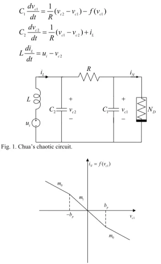
In this study, a Chua’s circuit [4], [5] with a double-scroll chaotic phenomenon as shown in Fig. 1 is studied. In Fig. 1, L is an inductor, and its corresponding

Manuscript received July 21, 2008. This work was supported in part by the National Science Council of Taiwan, R.O.C. through grant numbers NSC 97-2221-E-155-065-MY2.

(2)

current is represented as iL; C1 and C2 are capacitors

and their across voltages are repressed as vc1 and vc2; R

is a resistor; ui is a voltage source cascade with the

inductor L; ND represents a nonlinear Chua's diode with a

three-segment piecewise-linear characteristic of the capacitor voltage (vc1) and the diode current (iN) defined

by

1

0 1 1 0 1 1

( ) 1

( )[| | | |] 2

N c

c c p c p

i f v

m v m m v b v b

=

+ − + − −

(1)

where | |⋅ is the operator of absolute value; bp is a

predetermined boundary; m0 and m1 are the slopes in

the inside and outside regions of the boundary as shown in Fig. 2. According to Kirchhoff’s voltage and current laws, the state equations of the Chua’s circuit can be represented as

1

1 2 1 1

1

( ) ( )

c

c c c

dv

C v v f v

dt = R − − (2a)

2

2 1 2

1

( )

c

c c L

dv

C v v i

dt =R − + (2b)

2

L

i c

di

L u v

dt = − (2c)

1

C

2

C

R

L

i u

L i

+ +

− −c1

v

2

c

v ND

N i

Fig. 1. Chua’s chaotic circuit.

1

c v

1 ( )

N c

i =f v

p b

−

0

m

0

m

1

m

Fig. 2. Relation of capacitor voltage and diode current in non-linear resistor.

By introducing new variables x1=vc1, x2=vc2, and

3 L

x =i , then the system dynamics in (2) can be simplified as

1 ( 2 1) ( )1

x =a x −x −bf x (3a)

2 ( 1 2) 3

x = p x −x +qx (3b)

3 ( i 2)

x =r u −x (3c)

where a=1 / (RC1), b=1 /C1, p=1 / (RC2), q=1 /C2,

and r=1 /L. By considering the external disturbance and separating the normal parameters from the system dynamic, (3) can be expressed as

1 2 1 1

2 1 1 1

( )[ ] ( ) ( )

( ) ( )

n n

n n x

x a a x x b b f x

a x x b f x d

= + ∆ − − + ∆

− − +

(4a)

2 1 2 3

1 2 3 2

( )( ) ( )

( )

n n

n n x

x p p x x q q x

p x x q x d

= + ∆ − + + ∆

− + +

(4b)

3 2

2 3

(n )( i ) u

n x

x r r u x d

u r x d

= + ∆ − +

− +

(4c)

where an, bn, pn, qn and rn are the normal values of

a, b, p, q, and r, respectively, and ∆a, ∆b, ∆p, ∆q, and

r

∆ are their corresponding parameter variations; du is a

unpredictable external disturbance;

1 ( 2 1) ( )1

x

d = ∆a x −x − ∆bf x , dx2= ∆p x( 1−x2)+ ∆qx3 and

3 ( 2)

x i u

d = ∆r u −x +d denote respective lumped

uncertainties in (4); u=r un i is a new control input. The

control problem is to design a suitable control law to force the system states (x1,x2,x3) to track specific reference

commands ( x1r , x2r , x3r ) for eliminating chaotic

phenomena in the Chua’s circuit.

III. TOTAL SLIDING-MODE CONTROL

In order to control the Chua’s circuit effectively, a total sliding-mode control (TSMC) scheme as shown in Fig. 3 is introduced in this section. Define respective tracking errors as ex1= −x1 x1r, ex2=x2−x2r, and ex3=x3−x3r, in which

1r

x is the reference command voltage for the capacitor C1

(vc ref1 ); x2r(vc ref2 ) and x3r(iLref) are the corresponding

equilibrium points of x2 and x3 when x1=x1r. By only

considering the nominal system dynamics (i.e.,

1 2 3 0

x x x

d =d =d = ), x2r and x3r can be represented via

(4a) and (4b) as

1 1

2 1

( )

r n r

r r

n

x b f x

x x

a

+

(5a)

1 1

2 3

[ ( )]

n r n r

r r

n n n

p x b f x

x x

q a q

+

(5b)

From (4), one can organize the system dynamics in the following vector form:

1 1 1 1

2 2 2

3 3 3

0 0 ( )

0

0 0 1

n n x n

n n n x

n x

x a a x d b f x

x p p q x u d

x r x d

− −

⎡ ⎤ ⎡ ⎤ ⎡ ⎤ ⎡ ⎤ ⎡ ⎤

⎢ ⎥ ⎢₌ ₋ ⎥ ⎢ ⎥ ⎢ ⎥₊ ₊⎢ ⎥

⎢ ⎥ ⎢ ⎥ ⎢ ⎥ ⎢ ⎥ ⎢ ⎥

⎢ ⎥ ⎢ − ⎥ ⎢ ⎥ ⎢ ⎥ ⎢ ⎥

⎣ ⎦ ⎣ ⎦ ⎣ ⎦ ⎣ ⎦ ⎣ ⎦

(6a)

or

u

=A + +

x x h w_(6b)

where [ 1 2 3]

T

x x x

=

x _,

0

0 0

n n

n n n

n

a a

p p q

r

−

⎡ ⎤

⎢ ⎥

=_⎢ − _⎥

⎢ − ⎥

⎣ ⎦

A , and

[0 0 1]T

=

(3)

vector and is defined as

1 1 2 3

[ ( ) ]T

x n x x

d b f x d d

= −

w ₍₇₎

The TSMC presentation for the Chua’s circuit is divided into two main parts. The first part addresses performance design. The object is to specify the desired performance in terms of the nominal model, and it is referred to as baseline

model design. Following the baseline model design, the second part is the curbing controller design to totally eliminate the unpredictable perturbation effect from the parameter variations and external load disturbance so that the baseline model designs performance can be exactly assured.

1

s

1

n

s+p an

n

r 3

x d

2(c2) x v 3( )L

x i

1( c1) x v

( ) n

b f ⋅

1

x e

2

x e

3

x e

1r( c ref1 )

x v

2r( c ref2 )

x v

3r(Lref) x i

l

s

bs

u

cu

u

,

b w k

i

u

l s

1

n s+a

n r

n

q

2

x

d dx1

n p Chua’s Circuit

Total Sliding-Mode Control 1

s

1

n

s+p an

n

r 3

x d

2(c2) x v 3( )L

x i

1( c1)

x v

( )

n

b f ⋅

1

x e

2

x

e 3

x e

1r( c ref1 )

x v

2r( c ref2 )

x v

3r(Lref) x i

l s bs

u

cu

u

,

b w k

i

u

l s

1

n

s+a

n r

n

q

2

x

d dx1

n p Chua’s Circuit

Total Sliding-Mode Control Fig. 3. Block diagram of TSMC system.

A. Baseline Model Design

By differentiating (6b) with respect to time and considering the absence of the lumped uncertainty vector (i.e., w=0_{), one can rewrite the system dynamic via a} second-order vector form and devise in the control effort

bs

u in the baseline model design as follows:

u

=A +

x x h

(8)

[ ]

bs r v p

u =u h+ −Ax+x −Ke−K e ₍₉₎

where [ 1 2 3]

T

r ex ex ex

= −

e x x _{is a tracking error}

vector, in which [ 1 2 3]

T

r = xr xr xr

x _{is a reference}

command vector; 3 3

v R

× ∈

K and 3 3

p R

× ∈

K are positive

gain matrices; 1 3

R

+_∈ ×

h _{is the left penrose pseudo inverse}

of h_{, i.e.,} 1

( T ) T

+ ₌ −

h h h h _{. Substitute (9) into (8), one can}

obtain

0

v p

+K +K =

e e e ₍₁₀₎

Properly choosing the control gains in Kv and Kp, the

desired system dynamics such as rise time, overshoot, and settling time can be easily designed by this second-order vector. However, if the uncertainties occur, i.e., the parameters of the system are deviated from the nominal value or an external load disturbance is added into the system, the baseline model design can not guarantee the performance specified by (10). Moreover, the stability of the controlled system may be destroyed. To ensure the system performance designed by (10) despite the existence of the uncertain system dynamics, an auxiliary control

design is necessary.

B. Curbing Control Design

The baseline model dynamic shown in (10) can be rewritten in the state variable form as

cu =Acu cu

e e ₍₁₁₎

where 6 1

[ ]T

cu R

×

= ∈

e e e _and 3 3 3 3 6 6

cu

p v

R

× × ×

⎡ ⎤

=_⎢ _⎥∈

− −

⎣ ⎦

0 I

A

K K ,

in which I3 3× is an 3×3 identity matrix. Now, consider a

sliding surface as follows [10]:

0 ₀

( ) ( ) ( ) t ub

l ub cu ub cu T cu cu

cu

c

s t =c −c − ∂ dt

∂

∫

A

e e e

e (12)

where cub(ecu) is a scalar variable designed as

1 6 1 3

/ T [ ]

ub cu

c × + R×

∂ ∂e = 0 h ∈ _{, and}

0

cu

e _{is the initial state of}

cu

e _{. It is obvious that} ₍₀₎ ₀

l

s = and

( ) ub ub 0

l T cu T cu cu

cu cu

c c

s t =∂ −∂ =

∂e e ∂e A e

(13)

Thus, s tl( )=0 for all t≥0. Note that, since the function ( ) 0

l

s t = when t=0, there is no reaching phase as in the traditional sliding-mode control. If the Chua’s circuit subject to unknown parameter variations and external load disturbance is considered, the lumped uncertainly vector w

should be added in the system dynamics. Therefore, the system dynamic can be expressed as

( ) u

+ ₋ _{= +}

A +

(4)

It is apparent that the control shown in (9) can not ensure that (14) satisfies the baseline model design and s tl( )=0

for t>0. Thus, it is necessary to design an additional control such that the closed-loop dynamics of the controlled system is the same as the performance in the baseline model design. This is achieved by a control of the following form:

bs cu

u=u +u (15)

where ubs is the same as given by (9), and ucu is given as

sgn[ ( ) ] ( )

cu b l l

u = −w s t −ks t (16)

where sgn[ ]⋅ is a sign function; wb and k are positive

constants. The objectives of this controller ucu are twofold.

The first is to keep the controlled system dynamics on the surface s tl( )=0. That is, curb the system dynamics onto

( ) 0

l

s t = for all time. Thus, ucu is called a curbing

controller. Accordingly, the second objective is to guarantee that the closed-loop perturbed system has with the same performance shown in (10) as the baseline model design.

Substitute (9), (15) and (16) into (6b), the state variable form in (11) can be rewritten as follows:

[ ]

cu cu cu m ucu

+

=A + +

e e h h w ₍₁₇₎

where 6 1

3 1

[ ]T

m R

× ×

= 0 ∈

h h _{. Now,} _{( )} ₀

l

s t = when t=0. To maintain the state on the surface s tl( )=0 for all time,

on only needs to show that

( ) ( ) 0

l l

s t s t < if s tl( )≠0 (18)

By differentiating s tl( ) in (12) with respect to time and

using the error dynamic in (17), it yields

( )

{ [ ] }

ub ub

l T cu T cu cu

cu cu

ub

cu cu m cu cu cu

T cu

cu

c c

s t

c

u

+

∂ ∂

= −

∂ ∂

∂

= + + −

∂

= +

A

A A

e e

e h h w e

e

h w

(19)

Multiplying s tl( ) by (19) and inserting (7) into (19), one can obtain

3

2

3

( ) ( ) ( ) ( )

( ) ( )

( ) ( ) ( )

l l l cu l

l cu l x

l l b x

s t s t s t u s t

s t u s t d

ks t s t w d

+

= +

≤ +

= − − −

h w

(20)

If the condition of wb> dx3 holds, (20) can be rewritten

as

2

( ) ( ) ( ) 0

l l l

s t s t ≤ −ks t < (21)

Thus, the sliding mode can be assured throughout the whole control period. Note that, the value of wb can be

roughly determined to be a small positive constant for reducing the chattering phenomena in (16) because the term of −ks tl( ) via a large value of k is helpful for ensuring

( ) ( ) 0

l l

s t s t < in (20). The effectiveness of the proposed TSMC scheme is verified by the following numerical simulations.

Time(sec) Capacitor Voltage, vc1

Capacitor Voltage, vc2 Inductor Current,iL

(a) (b)

Double-scroll

Ca

p

ac

ito

r V

o

lta

g

e,

vc2

Capacitor Voltage,vc1

Time(sec) Time(sec)

(c) (d)

V

V _mA

Time(sec) Capacitor Voltage, vc1

Capacitor Voltage, vc2 Inductor Current,iL

(a) (b)

Double-scroll

Ca

p

ac

ito

r V

o

lta

g

e,

vc2

Double-scroll

Ca

p

ac

ito

r V

o

lta

g

e,

vc2

Time(sec) Time(sec)

(c) (d)

V

V _mA

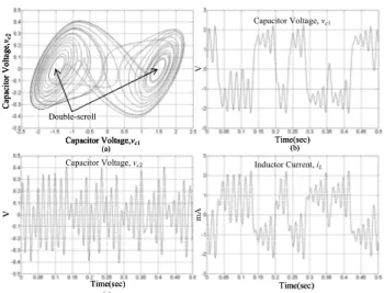
Fig. 4. Numerical simulations of open-loop examination for Chua’s circuit: (a) Phase plane trajectory, vc1−vc2; (b) Capacitor voltage, vc1; (c)

Capacitor voltage, vc2; (d) Inductor current, iL.

IV. NUMERICAL SIMULATIONS

In order to exhibit the merits of the total sliding-mode control (TSMC) system, a conventional sliding-mode control (CSMC) scheme introduced from [12] is also examined in this study. In this CSMC strategy, a conventional sliding-surface vector is defined as

0

( ) t

c t = +

∫

G dt

s e e ₍₂₂₎

where 3 3

R×

∈

G is a positive-definite gain matrix.

According to the standard derivation procedure [6], [7], [12], the CSMC law can be represented as

{ sgn[ ( )]}

CSMC r c c

u =h+ x −Ax−Ge−w s t ₍₂₃₎

where wc is the upper bound of the lumped uncertainty

vector, i.e., w <wc, in which ⋅ is the Euclidean norm.

All numerical simulations are carried out using Windows packaged Matlab 6.5 edition software. The circuit specifications of a Chua’s circuit are summarized as follows:

Sampling time T =25 sµ ; Control time Tr =50 sµ ;

Inductor L=0.707H;

Capacitor C1=0.55 Fµ ;

2 4.95 F

C = µ ;

Resistor 1.428kR= Ω;

Chua's diode m0 = −0.5 mA V;

1 0.8 mA V

m = − ;

1V

p

b =

Moreover, the initial condition for the capacitor voltage is set at vc1(0)=0.5V. In addition, the control parameters of

CSMC and TSMC systems are given as

1 0 0

0 1 0

0 240 30000

v

⎡ ⎤

⎢ ⎥

= ⎢ ⎥

⎢ ⎥

⎣ ⎦

K ,

6 7

1 0 0

0 1 0

0 10 5 10

p

⎡ ⎤

⎢ ⎥

= ⎢ ⎥

⎢ × ⎥

⎣ ⎦

(5)

1 0 0

0 1 0

0 20 2000

⎡ ⎤

⎢ ⎥

= ⎢ ⎥

⎢ ⎥

⎣ ⎦

G , wb=0.01, k=100,

8

c

w = , x1r =2 (24)

All the parameters in (24) are chosen to achieve superior transient control performance in numerical simulations by considering the possible occurrence of operational conditions and the limitation of control efforts.

Control Voltage, ui

V

Cap

ac

ito

r Vo

lta

g

e,

vc2

Capacitor Voltage, vc1

Inductor Current, iL Capacitor Voltage Command, x1r

V

V _mA

(2, 0.1436)

Inductor Current Command, x3r Time(sec)

Time(sec)

(a) (b)

(d) Capacitor Voltage,vc1

Time(sec) (c)

Time(sec) (e) Capacitor Voltage Command, x2r

Control Voltage, ui

V

Cap

ac

ito

r Vo

lta

g

e,

vc2

V

V _mA

(2, 0.1436)

Time(sec)

(a) (b)

Time(sec) (c)

Time(sec) (e) Capacitor Voltage Command, x2r

Fig. 5. Numerical simulations of CSMC scheme for Chua’s circuit at case 1: (a) Phase plane trajectory, vc1−vc2; (b) Tracking response of capacitor

voltage vc1; (c) Tracking response of capacitor voltage vc2; (d) Tracking

response of inductor current iL; (e) Control voltage, ui.

In order to investigate the robust characteristics of the proposed TSMC system, two examined cases are considered: Case 1 is the normal condition (i.e.,

1 2 3 0

x x x

d =d =d = ); Case 2 is the disturbance condition

(i.e., dx1=0.2 cos(201 ) 0.5 cos(53πt + πt)

,

2 0.2cos(201 t)+0.5cos(53 t)

x

d = π π , and

3 2cos(201 t)+5cos(53 t)

x

d = π π occurred at beginning).

Numerical simulations of the open-loop examination for the Chua’s circuit are depicted in Fig. 4. From Fig. 4(a), one can see that the phase palne trajectory vc1−vc2

describe a double-scroll Chua’s attractor. The corresponding responses of the capacitor voltages (vc1 and

2

c

v ) and inductor current (iL) are depicted in Fig. 4(b)−(d),

respectively. Comparative simulations of the CSMC scheme at cases 1 and 2 are depicted in Figs. 5 and 6, respectively. At case 1, one can see that the phase trajectory

1 2

c c

v −v as shown in Fig. 5(a) can be controlled to its command (2, 0.1436), and the responses of the capacitor

voltage (vc1 and vc2) as shown in Fig. 5(b) and (c) can

arrive at their command voltages ( x1r and x2r ),

respectively. However, the chattering control voltage in Fig. 5(e) caused by the sign function in (23) results in the shaking response of the inductor current in Fig. 5(d). At case 2, the phase trajectory vc1−vc2 as shown in Fig. 6(a)

also can be controlled to its command (2, 0.1436), but the trajectory in comparison with the one in Fig. 5(a) is obviously sensitive to external disturbances. Besides, the responses of the capacitor voltages and inductor current as shown in 6(b)−(d) become slow, and their corresponding tracking responses degenerate due to the occurrence of external disturbances.

Control Voltage, ui

V

C

ap

ac

ito

r V

o

lt

a

g

e,

vc2

V

Capacitor Voltage Command, x1r

Capacitor Voltage Command, x2r

V

Inductor Current, iL

mA

(2, 0.1436)

Time(sec)

(a) (b)

Time(sec) (c)

Time(sec) (e)

Fig. 6. Numerical simulations of CSMC scheme for Chua’s circuit at case 2: (a) Phase plane trajectory, vc1−vc2; (b) Tracking response of capacitor

(6)

Control Voltage, ui

V

Ca

p

aci

to

r Vo

lt

a

g

e,

vc2

Capacitor Voltage,vc2 _{Inductor Current,}_i

L Capacitor Voltage Command, x2r

Inductor Current Command, x3r Capacitor Voltage Command, x1r

V

V _mA

(2, 0.1436)

Time(sec)

(a) (b)

(d)

Time(sec)

(c)

Time(sec)

(e)

Fig. 7. Numerical simulations of TSMC strategy for Chua’s circuit at case 1: (a) Phase plane trajectory, vc1−vc2; (b) Tracking response of capacitor

Control Voltage, ui

V

Time(sec)

(a) (b)

(d)

Cap

acito

r V

o

lta

ge,

vc2

Inductor Current Command, x3r Capacitor Voltage Command, x1r

V

mA

(2, 0.1436)

Time(sec) (c)

Time(sec) (e)

Fig. 8. Numerical simulations of TSMC strategy for Chua’s circuit at case 2: (a) Phase plane trajectory, vc1−vc2; (b) Tracking response of capacitor

V. CONCLUSIONS

This study has successfully developed a total sliding-mode control (TSMC) system to handle a Chua’s chaotic circuit. Numerical simulations are presented to illustrate the effectiveness of the proposed TSMC scheme, and its superiority is indicated in comparison with a conventional sliding-mode control (CSMC) system. According to the simulated results, it is obvious that the chattering control efforts in the CSMC can be greatly alleviated, and the TSMC has a total sliding motion without a reaching phase so that the control performances are less sensitive to system uncertainties. Consequently, the proposed TSMC scheme is more suitable for the state control of the Chua’s chaotic circuit than the CSMC system.

REFERENCES

[1] K. T. Alligood and T. Sauer, Chaos. New York: Springer, 1996.

[2] G. P. Jiang and W. X. Zheng, “Chaos control for a class of chaotic systems using PI-type state observer approach,” Chaos, Solitons & Fractals, vol. 21, no. 1, pp. 93-99, 2004.

[3] J. F. Chang, M. L. Hung, Y. S. Yang, T. L. Liao, and J. J. Yan, “Controlling chaos of the family of Rössler systems using sliding mode control,” Chaos, Solitons & Fractals, doi:10.1016/j.chaos.2006.09.051, 2006. [4] T. Matsumoto, L. O. Chua, and M. Komuro, “The

double scroll,” IEEE Trans. Circuits Syst. I, vol. 32, pp. 797-818, 1985.

[5] H. Puebla, J. Alvarez-Ramirez, and I. Cervantes, “A simple tracking control for Chua’s circuit,” IEEE Trans. Circuits Syst. I, vol. 50, no. 2, pp. 280-284, 2003. [6] J. J. E. Slotine and W. Li, Applied Nonlinear Control.

New Jersey: Prentice Hall, 1991.

[7] K. J. Astrom and B. Wittenmark, Adaptive Control. New York: Addison-Wesley, 1995.

[8] Z. Lu, L. S. Shieh, and G. R. Chen, “On robust control of uncertain chaotic systems: a sliding-mode synthesis via chaotic optimization,” Chaos, Solitons & Fractals, vol. 18, no. 4, pp. 819-827, 2003.

[9] W. Gao and J. C. Hung, “Variable structure control for nonlinear systems: a new approach,” IEEE Trans. Ind. Electron., vol. 40, no. 1, pp. 2-22, 1993.

[10] R. J. Wai, “Adaptive sliding-mode control for induction servomotor drive,” IEE Proc. Electr. Power Appl., vol. 147, no. 6, pp. 553-562, 2000.

[11] J. J. Yan, Y. S. Yang, T. Y. Chiang, and C. Y. Chen, “Robust synchronization of unified chaotic systems via sliding mode control,” Chaos, Solitons & Fractals, vol. 34, no. 3, pp. 947-954, 2007.