The GOME-2 instrument on the Metop series of satellites: instrument design, calibration, and level 1 data processing – an overview

(1)

AMTD

8, 8645–8700, 2015

The GOME-2 instrument on the

Metop series of satellites

R. Munro et al.

Title Page

Abstract Introduction

Conclusions References

Tables Figures

◭ ◮

Back Close

Full Screen / Esc

Printer-friendly Version Interactive Discussion

Discussion

P

a

per

|

Discussion

P

a

per

|

Discussion

P

a

per

|

Discussion

P

a

per

|

Atmos. Meas. Tech. Discuss., 8, 8645–8700, 2015 www.atmos-meas-tech-discuss.net/8/8645/2015/ doi:10.5194/amtd-8-8645-2015

This discussion paper is/has been under review for the journal Atmospheric Measurement Techniques (AMT). Please refer to the corresponding final paper in AMT if available.

The GOME-2 instrument on the Metop

series of satellites: instrument design,

calibration, and level 1 data processing –

an overview

R. Munro1, R. Lang1, D. Klaes1, G. Poli1, C. Retscher1, R. Lindstrot1, R. Huckle1, A. Lacan1, M. Grzegorski1, A. Holdak1, A. Kokhanovsky1, J. Livschitz2, and M. Eisinger3

1

EUMETSAT, Eumetsat-Allee 1, Darmstadt, Germany

2

European Space Agency – European Space Research & Technology Centre (ESA-ESTEC), Noordwijk, the Netherlands

3

European Space Agency – European Centre for Space Applications and Telecommunications (ESA-ECSAT), Didcot, Oxfordshire, UK

Received: 28 April 2015 – Accepted: 15 June 2015 – Published: 11 August 2015

Correspondence to: R. Munro (rosemary.munro@eumetsat.int)

(2)

AMTD

8, 8645–8700, 2015

R. Munro et al.

Title Page

Tables Figures

◭ ◮

Back Close

Full Screen / Esc

Discussion

P

a

per

|

Discussion

P

a

per

|

Discussion

P

a

per

|

Discussion

P

a

per

|

Abstract

The Global Ozone Monitoring Experiment-2 (GOME-2) flies on the Metop series of satellites, the space component of the EUMETSAT Polar System. In this paper we will provide an overview of the instrument design, the on-ground calibration and charac-terisation activities, in-flight calibration, and level 0 to 1 data processing. The quality of

5

the level 1 data is presented and points of specific relevance to users are highlighted. Long-term level 1 data consistency is also discussed and plans for future work are out-lined. The information contained in this paper summarises a large number of technical reports and related documents containing information that is not currently available in the published literature. These reports and documents are however made available

10

on the EUMETSAT web pages (http://www.eumetsat.int) and readers requiring more details than can be provided in this overview paper will find appropriate references at relevant points in the text.

1 The Global Ozone Monitoring Experiment 2 (GOME-2) instrument

The Global Ozone Monitoring Experiment-2 (GOME-2) is an improved version of the

15

Global Ozone Monitoring Experiment which flew on the second European Remote Sensing Satellite (GOME-1/ERS-2) (Munro, 2006). For a summary of improvements please see Munro, 2006. GOME-2 flies on the Metop series of satellites. The Metop satellites form the space component of the EUMETSAT Polar System and fly in a sun-synchronous orbit, at an altitude of approximately 820 km, and with a descending

20

node equator crossing local solar time of 9:30. The first Metop satellite, Metop-A, was launched on 19 October 2006. After a successful commissioning phase, Metop-B, on 24 April 2013, replaced Metop-A as EUMETSAT’s prime operational polar-orbiting satellite. Metop-A and Metop-B now fly in a tandem operations configuration on the same orbit but separated by 48.93 min. Metop-C is currently planned for launch in

(3)

AMTD

8, 8645–8700, 2015

R. Munro et al.

Title Page

Tables Figures

◭ ◮

Back Close

Full Screen / Esc

Discussion

P

a

per

|

Discussion

P

a

per

|

Discussion

P

a

per

|

Discussion

P

a

per

|

2018. For more information about the EUMETSAT Polar System and the Metop series of satellites see Klaes et al., 2007.

GOME-2 is an optical spectrometer fed by a scan mirror which enables across-track scanning in nadir, as well as sideways viewing for polar coverage and instrument char-acterisation measurements using the moon (Callies et al., 2000). This scan mirror can

5

also be directed towards internal calibration sources or towards a diffuser plate for calibration measurements using the sun. GOME-2 senses the Earth’s backscattered radiance and extraterrestrial solar irradiance in the ultraviolet and visible part of the spectrum (240–790 nm) at a high spectral resolution of 0.26–0.51 nm. The instrument comprises four main optical channels (Focal Plane Assemblies – FPAs) which focus the

10

spectrum on linear detector arrays of 1024 pixels each, and two Polarisation Measure-ment Devices (PMDs) containing the same type of arrays for measureMeasure-ment of linearly polarised intensity in two perpendicular directions. The PMDs are required because GOME-2 is a polarisation sensitive instrument. Therefore, the intensity calibration of GOME-2 has to take account of the polarisation state of the incoming light using

in-15

formation from the PMDs. The PMD measurements are performed at lower spectral resolution, but at higher spatial resolution than the main science channels, which also facilitates sub-pixel determination of cloud coverage.

The footprint size is 80 km×40 km for main science channel data for a nominal swath

width of 1920 km. The polarisation data are down-linked in 15 spectral bands covering

20

the region from 312–800 nm for both polarisation directions with a footprint of 10 km×

40 km also for a nominal swath width of 1920 km.

The recorded spectra are used to derive a detailed picture of the total atmospheric content of ozone and the vertical ozone profile in the atmosphere. They also provide accurate information on the total column amount of nitrogen dioxide, sulphur dioxide,

25

(4)

AMTD

8, 8645–8700, 2015

R. Munro et al.

Title Page

Tables Figures

◭ ◮

Back Close

Full Screen / Esc

Discussion

P

a

per

|

Discussion

P

a

per

|

Discussion

P

a

per

|

Discussion

P

a

per

|

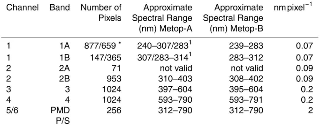
The GOME-2 instrument was developed by Selex Galileo in Florence, Italy, under a joint contract from EUMETSAT and ESA. The main instrument GOME-2 characteris-tics are summarised in Table 1.

1.1 GOME-2 optical layout

The four main channels (detectors) of the GOME-2 instrument provide continuous

5

spectral coverage of the wavelengths between 240 and 790 nm with a spectral res-olution full width at half maximum (FWHM) between 0.26 and 0.51 nm. Channel char-acteristics for GOME-2 on Metop-A (Flight Model 3 – FM3) and GOME-2 on Metop-B (Flight Model 2 – FM2) are listed in Table 2. Wavelength values are indicative only and will depend on spectral calibration. Spectral resolution (FWHM) varies slightly across

10

each main channel, the values given are channel averages. In the overlap regions be-tween the main science channels, the wavelengths indicate the 10 % overlap points. E.g., at 310 nm, 10 % of the signal is registered in channel 2, and 90 % in channel 1. At 314 nm, 10 % of the signal is registered in channel 1, and 90 % in channel 2. Note however that the calibrated level 1 data are generally not fully valid for the whole

15

overlap region. The spectral extent of the valid data is not static and typically, but not always, extends approximately to the 50 % overlap point, depending on the quality of calibration parameters and corrections. A detailed description of the valid ranges for all operational GOME-2 flight models can be found in EUMETSAT, 2014a.

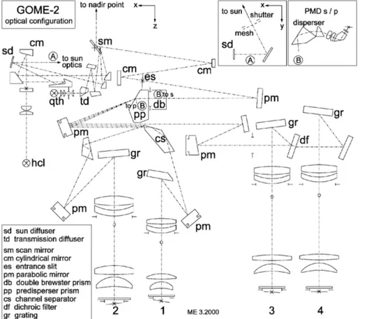
The optical configuration of the instrument is shown in Fig. 1. Light enters the two

20

mirror telescope system via the scan mirror. The telescope projects the light beam onto the slit, which determines the instantaneous field-of-view (IFOV) of 0.28◦

×2.8◦

(across-track×along-track). After it has passed the slit, the beam is collimated again

and enters a double Brewster prism for partial split-o_ffto PMD-S, followed by the pre-disperser prism which has two functions. Brewster reflection at the back of the prism

25

(5)

AMTD

8, 8645–8700, 2015

R. Munro et al.

Title Page

Tables Figures

◭ ◮

Back Close

Full Screen / Esc

Discussion

P

a

per

|

Discussion

P

a

per

|

Discussion

P

a

per

|

Discussion

P

a

per

|

and 3 and 4, respectively. The separation between channels 3 and 4 is performed by a dichroic filter.

A grating in each channel then further disperses the light, which is subsequently fo-cused onto the detector array. Each PMD channel contains a dispersion prism and two additional folding prisms and collimating lenses. PMD-P measures intensity polarised

5

parallel to the spectrometer’s slit, and PMD-S measures intensity polarised perpendic-ular to the spectrometer’s slit. The two PMD channels are designed to ensure maximum similarity in their optical properties. The wavelength dependent dispersion of the prisms causes a much higher spectral resolution in the ultraviolet than in the red part of the spectrum.

10

In order to reduce the dark signal, the detectors of the main channels are actively cooled by Peltier elements in a closed control loop to temperatures around 235 K. The FPA temperatures for all main channels are very stable due to the closed loop cooling configuration. The PMDs are cooled by Peltier elements in an open loop configuration and have detector temperatures around 231 K (the actual value depends on in-orbit

15

instrument temperature and PMD cooler settings). PMD temperatures vary somewhat and are closely linked to the optical bench temperature of the instrument. The optical bench is not temperature stabilised and its operational temperature is between 275 and 280 K.

In order to calculate the transmission of the atmosphere, which contains the

rele-20

vant information on trace gas concentrations, the solar radiation incident on the atmo-sphere must be known. For this measurement a solar viewing port is located on the flight-direction side of the instrument. When this port is opened, sunlight is directed via a∼40◦incidence mirror to a diffuser plate. Light scattered from this plate, or in general,

light from other calibration sources such as the PtCrNeAr Spectral Light Source (SLS)

25

(6)

AMTD

8, 8645–8700, 2015

R. Munro et al.

Title Page

Tables Figures

◭ ◮

Back Close

Full Screen / Esc

Discussion

P

a

per

|

Discussion

P

a

per

|

Discussion

P

a

per

|

Discussion

P

a

per

|

Diodes (LEDs) which are located in front of the detectors to monitor the pixel-to-pixel gain.

1.2 GOME-2 band definitions and integration times

1.2.1 Main Focal Plane Assembly (FPA) band settings

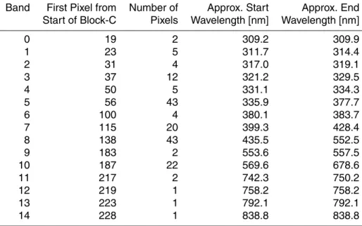
The GOME-2 channels can be separated into different bands. The operational band

5

settings are provided in Table 3. Note that the separation between band 1A and band 1B, for GOME-2 on Metop-A, was shifted on 10 December 2008 from 307 to 283 nm to be consistent with the settings used for both ERS-2/GOME-1 and EN-VISAT/SCIAMACHY. GOME-2 on Metop-B has also used these updated settings since the beginning of operations. Each band can be operated at different integration times

10

which can also vary over the orbit. The actual integration times used and thus the ground pixel size, depend on the light intensity. Nominal integration times in band 1A are 1.5 s (6 s at high solar zenith angles) and 0.1875 s for band 1B to 4 (1.5 and 0.75 s at high SZA). For details on the exact integration times per band during one instrument timeline series, we refer to the GOME-2 monitoring pages in the timelines sub-section

15

at gome.eumetsat.int.

1.2.2 Polarisation Measurement Device (PMD) band settings

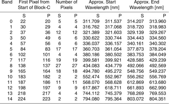
For Earthshine measurements, the 256 used detector pixels of both PMD devices (for details we refer to EUMETSAT, 2014b) are spectrally co-added on board into 15 PMD-Spectral bands. Before 11 March 2008, both PMD detectors (PMD-S and PMD-P) of

20

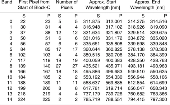
GOME-2 on Metop-A used the same band settings, defined as a function of detector pixel, as listed in Table 4. On 11 March 2008 in orbit 7227, updated PMD band set-tings, with different settings for PMD-S and PMD-P were uploaded to the instrument in order to improve the spectral co-registration of both PMDs and to optimise the utility of PMD bands for level 2 data retrieval (Table 5). For GOME-2 on Metop-B the PMD

(7)

AMTD

8, 8645–8700, 2015

R. Munro et al.

Title Page

Tables Figures

◭ ◮

Back Close

Full Screen / Esc

Discussion

P

a

per

|

Discussion

P

a

per

|

Discussion

P

a

per

|

Discussion

P

a

per

|

band settings (Table 6) have not been changed since the beginning of operational data production.

For more details on the PMD calibration and PMD band settings we refer to EUMET-SAT 2013 and EUMETEUMET-SAT 2014c.

1.3 On-ground calibration and characterisation

5

The GOME-2 instrument was built by an industrial team led by Selex Galileo (I) with support from Laben (I), TNO-TPD (NL), Arcom Space (DK), Innoware (DK) and Fi-navitec (FIN) where TNO-TPD are responsible for the calibration and characterisation of the instrument.

Calibration and characterisation measurements are taken during an extensive

on-10

ground campaign. The detailed characterisation measurements are fully described in TPD, 2003 and TPD, 2004a. Characterisation measurements are post-processed to provide calibration key data files which are documented both in terms of content and format in TNO, 2011a, b, and 2012. A sub-set of the calibration key data are a required input to the GOME-2 level 0 to 1 processor e.g. the radiance, irradiance and polarisation

15

response of the instrument.

For a full list of those key data used by the GOME-2 level 0 to 1b processing chain see EUMETSAT, 2014b. Other key data describe aspects of the on-ground behaviour of the instrument which will also be measured in-orbit using on-board calibration targets e.g. dark signal performance, pixel-to-pixel gain, spectral calibration, and etalon.

20

Additionally, the slit-function shape must be characterised at sub-pixel resolution pre-flight, as this cannot be determined adequately from information available in-flight. As a result additional slit function characterisation data were also acquired during the on-ground calibration and characterisation campaign (TPD, 2004b). These data were fur-ther analysed by TNO-TPD and the Rufur-therford Appleton Laboratory to provide

addi-25

(8)

AMTD

8, 8645–8700, 2015

R. Munro et al.

Title Page

Tables Figures

◭ ◮

Back Close

Full Screen / Esc

Discussion

P

a

per

|

Discussion

P

a

per

|

Discussion

P

a

per

|

Discussion

P

a

per

|

function characterisation data are available from the GOME-2 monitoring pages in the documentation sub-section at gome.eumetsat.int.

1.4 In-flight characterisation and calibration

A range of in-flight characterisation and calibration activities are carried out routinely during GOME-2 operations. These activities provide input to level 0 to 1b processing,

5

in addition to the calibration key data measured on-ground, to ensure the generation of high quality spectrally and radiometrically calibrated radiance and irradiance data and continuous monitoring of instrument performance.

Calibration activities interleaved with nominal observations comprise dark signal measurements performed every orbit in eclipse and sun calibration measurements

per-10

formed once per day at sunrise in the Northern Hemisphere. The sun calibration uses one of the on-board stored timelines which includes in addition to the sun measure-ments itself, both a wavelength calibration and a radiometric calibration. The timeline must be triggered such that the instrument is commanded into SUN observation mode prior to the sun appearing in the instrument field of view. For the remainder of the orbit

15

the timeline consists of nadir scanning observations.

In addition, regular monthly calibration activities take place. The frequency is deter-mined by the expected change in the mean optical bench temperature, resulting from seasonal variations in the external heat load from the sun, and long-term degradation of thermo-optical surfaces. Although it is primarily the wavelength calibration that is

ex-20

(9)

AMTD

8, 8645–8700, 2015

R. Munro et al.

Title Page

Tables Figures

◭ ◮

Back Close

Full Screen / Esc

Discussion

P

a

per

|

Discussion

P

a

per

|

Discussion

P

a

per

|

Discussion

P

a

per

|

1.5 GOME-2 observation modes

1.5.1 Earth observation modes

Earth observation (or “Earthshine”) modes are those modes where the earth is in the field of view of GOME-2. They are usually employed on the dayside of the earth (sunlit part of the orbit). The scan mirror can be at a fixed position (static modes), or scanning

5

around a certain position (scanning modes). All internal light sources are switched o_ff and the solar port of the calibration unit is closed.

– Nadir scanning.This is the mode in which GOME-2 is operated most of the time. The scan mirror performs a nadir swath as described above.

– Nadir static.The scan mirror is pointing towards nadir. This mode is typically used

10

during the monthly calibration. It is valuable for validation and long-loop sensor performance monitoring purposes.

1.5.2 Calibration modes

In-orbit instrument calibration and characterisation data are acquired in the various calibration modes. They are usually employed during eclipse with the exception of the

15

solar calibration which is performed at sunrise. Both internal (WLS, SLS, LED) and external (sun, moon) light sources can be employed. The various sources are selected by the scan mirror position.

– Dark. The scan mirror points towards the GOME-2 telescope. All internal light sources are switched offand the solar port is closed. Dark signals are typically

20

measured every orbit during eclipse.

– Sun (over diffuser). The scan mirror points towards the diffuser. All internal light sources are switched off and the solar port is open. Solar spectra are typically acquired once per day at the terminator in the Northern Hemisphere. The Sun Mean Reference (SMR) spectra are derived from this mode.

(10)

AMTD

8, 8645–8700, 2015

R. Munro et al.

Title Page

Tables Figures

◭ ◮

Back Close

Full Screen / Esc

Discussion

P

a

per

|

Discussion

P

a

per

|

Discussion

P

a

per

|

Discussion

P

a

per

|

– White light source (direct).The scan mirror points towards the WLS output mirror. The WLS is switched on and the solar port is closed. Etalon (and optionally Pixel-to-Pixel Gain (PPG) calibration) data are derived from this mode.

– Spectral light source (direct).The scan mirror points towards the SLS output mir-ror. The SLS is switched on and the solar port is closed. Wavelength calibration

5

coefficients are derived from this mode.

– Spectral light source over diffuser. The scan mirror points towards the diffuser. The SLS is switched on and the solar port is closed. Light from the SLS reaches the scan mirror via the di_ffuser. This mode is intended to be employed for in-orbit monitoring of the sun diffuser reflectivity. In practise, however, this instrument

10

mode has not been particularly useful as the SLS has proven to be unstable for the long integration times required to measure over the sun diffuser. Analysis of these measurements has only been used to provide a rough estimate of the upper boundary for diffuser degradation.

– LED. The scan mirror points towards the GOME-2 telescope. The LEDs are

15

switched on and the solar port is closed. Pixel-to-pixel gain (PPG) calibration data are derived from this mode.

– Moon.The scan mirror points towards the moon (typical viewing angles are+70 to

+85◦_{). As the spacecraft moves along the orbit, the moon passes the GOME-2 slit} within a few minutes. This mode can be employed only if geometrical conditions

20

(lunar azimuth, elevation and pass angle) allow, which typically occur a few times per year.

1.6 GOME-2 instrument operations plan

The default swath width of the scan is 1920 km which enables global coverage of the Earth’s surface within 1.5 days. The scan mirror speed can be adjusted such that,

25

(11)

AMTD

8, 8645–8700, 2015

R. Munro et al.

Title Page

Tables Figures

◭ ◮

Back Close

Full Screen / Esc

Discussion

P

a

per

|

Discussion

P

a

per

|

Discussion

P

a

per

|

Discussion

P

a

per

|

dimension of the instantaneous field-of-view (IFOV) is∼40 km which is matched with

the spacecraft velocity such that each scan closely follows the ground coverage of the previous one. The IFOV across-track dimension is∼4 km. For the 1920 km swath,

the maximum temporal resolution of 187.5 ms for the main channels (23.4 ms for the PMD channels) corresponds to a maximum ground pixel resolution (across track x

5

along track) of 80 km×40 km (10 km×40 km for the PMDs) in the forward scan. Since

15 July 2013, both GOME-2 instruments on board Metop-A and Metop-B have been operated in tandem with the swath width of GOME-2 on Metop-A changed to 960 km, while GOME-2 on Metop-B remains with the full swath width of 1920 km. This results in a ground pixel size of 40 km×40 km for GOME-2 on Metop-A main science channels 10

(5 km×40 km for the PMDs) and 80 km×40 km for GOME-2 on Metop-B main science

channels (10 km×40 km for the PMDs).

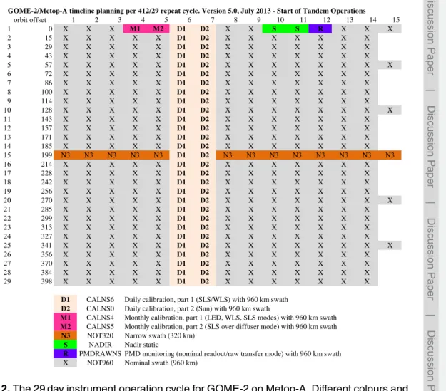
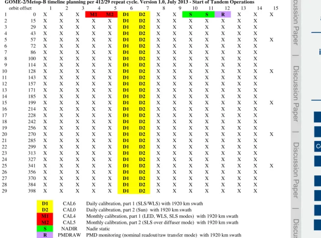
The 29 day instrument operations plans for Metop-A and Metop-B are shown in Figs. 2 and 3. The monthly calibration sequence is activated for both instruments on the same day with two nadir static orbits (no scanning) followed by one orbit during which

15

the PMD data is down-linked at full spectral resolution (256 channels for both PMDs) but with a reduced number of readouts (12 read-outs in forward and 4 read-outs in backward scanning direction whilst retaining nominal spatial resolution for PMDs, i.e. with gaps in between the read-outs). This configuration is called the monthly PMD RAW read-out configuration. GOME-2 on Metop-A is also configured to operate once per

20

month with a reduced swath width of 320 km. For further information see the GOME-2 monitoring pages in the timelines sub-section at gome.eumetsat.int. For more details on GOME-2 operations and the instrument settings, see EUMETSAT, 2014a.

1.7 GOME-2 data packet structure and synchronisation of measurements

A basic concept in the operation of the GOME-2 instrument is that of the “scan”. A scan

25

(12)

AMTD

8, 8645–8700, 2015

R. Munro et al.

Title Page

Tables Figures

◭ ◮

Back Close

Full Screen / Esc

Discussion

P

a

per

|

Discussion

P

a

per

|

Discussion

P

a

per

|

Discussion

P

a

per

|

fly-back (subsets 12 to 15). In the static and calibration modes the scan mirror does not move, but the data packet structure is identical to the scanning mode.

In the default measuring mode, the nadir scan, the scan mirror sweeps in 4.5 s (12 subsets) from negative (East) to positive (West) viewing angles, followed by a fly-back of 1.5 s (the last 4 subsets) back to negative viewing angles as shown in Fig. 4.

5

GOME-2 creates a Science Data Packet every 375 ms. One packet contains one UTC time stampt₀, four scanner positions (sampling 93.75 ms), at most two readouts of the main channels (effective integration time 187.5 ms), at most 16 readouts of the PMD bands (integration time 23.4375 ms).

Their relative timing is shown in Fig. 5. The first scanner position is given at time

10

t0+ ∆tSM (the time delta for the scan mirror between one data packet and the next).

At the same time, the first main channel readout and the first PMD readout within the packet start. The readout time is 45.78 µs for one detector pixel, i.e. 46.875 ms for a complete main channel readout (1024 detector pixels), and 11.72 ms for a readout of PMD blocks BCD (256 detector pixels, see EUMETSAT, 2014a.). Any readout operation

15

resets a detector pixel, and therefore marks theend of the integration for this detector pixel. The integration starts at thepreviousreadout.

The readout sequence for each detector can be programmed to be either from short to long wavelengths (“up”) or from long to short wavelengths (“down”).

2 GOME-2 Level 0 to 1 data processing

20

(13)

AMTD

8, 8645–8700, 2015

R. Munro et al.

Title Page

Tables Figures

◭ ◮

Back Close

Full Screen / Esc

Discussion

P

a

per

|

Discussion

P

a

per

|

Discussion

P

a

per

|

Discussion

P

a

per

|

2.1 Level 0 to 1a processing

The level 0 to 1a processing comprises both the determination of geolocation informa-tion on a fixed time grid, and the determinainforma-tion of applicable calibrainforma-tion parameters. From measurements of the various calibration sources encountered during each run of the processor, new calibration constants are calculated and written into an in-flight

5

calibration data file. They are also retained in memory for use in processing those data acquired after the satellite comes out of the dark side of the orbit and before the next dump. Updated calibration parameters are available for immediate use. Cali-bration parameters are stored for the lifetime of the mission. The caliCali-bration constant determination comprises:

10

– dark current correction

– pixel-to-pixel gain correction

– determination of spectral calibration parameters

– etalon correction

– determination of stray light correction factors for the sun and polarisation

mea-15

surements

– determination of the solar mean reference spectrum, and atmospheric polarisa-tion state

The geolocation of the measurements is calculated from the appropriate orbit and attitude information, and time correlation information in the level 0 data stream. Note,

20

any application of calibration parameters in the level 0 to 1a processing should be regarded as interim, to facilitate the generation of new calibration parameters and cor-rection factors. There is no application of calibration parameters to main channel earth observation measurements. The output of the level 0 to 1a processor is formatted into the level 0 and 1a products as specified in EUMETSAT, 2010 and 2014d.

(14)

AMTD

8, 8645–8700, 2015

R. Munro et al.

Title Page

Tables Figures

◭ ◮

Back Close

Full Screen / Esc

Discussion

P

a

per

|

Discussion

P

a

per

|

Discussion

P

a

per

|

Discussion

P

a

per

|

2.2 Level 1a to 1b processing

The level 0 to 1b processing comprises the calculation of geolocation parameters for the actual integration time of each measurement, determination of stray light correc-tion factors for the Earthshine measurements, and the conversion of the raw binary readouts on the level 1a data stream to calibrated radiance and irradiance data. Cloud

5

parameters are also determined. Furthermore, calibrated measurements from the on-board calibration sources, and the sun and moon are available in the level 1b product. Level 1b data are formatted as specified in EUMETSAT, 2010 and 2014d.

3 GOME-2 Level 0 to 1 Algorithms

3.1 Geolocation and synchronisation of main channel and PMD data

10

Basic geolocation parameters such as the sub-satellite point and solar angles at the satellite are calculated for all measurement modes. In addition, mode-specific geolo-cation parameters are calculated for earth, sun, and moon modes as follows:

– Earth mode.Solar and line-of-sight zenith and azimuth angles at a given height, corner and centre coordinates (latitude/longitude) of the ground pixel at ground

15

level, satellite height, and earth radius.

– Sun mode.Distance between satellite and sun and relative speed of satellite and sun.

– Moon mode. Lunar elevation and azimuth angles, sun-moon distance, satellite-moon distance, lunar phase angle, illuminated fraction of lunar disk.

20

(15)

AMTD

8, 8645–8700, 2015

R. Munro et al.

Title Page

Tables Figures

◭ ◮

Back Close

Full Screen / Esc

Discussion

P

a

per

|

Discussion

P

a

per

|

Discussion

P

a

per

|

Discussion

P

a

per

|

the position, relative to the ground pixel, of points for which geolocation information is provided in the GOME-2 level 1b product.

Note that geolocation information is provided in the GOME-2 level 1b product only for the first detector pixel of each channel (EUMETSAT, 2010 and 2014d). Therefore for a proper assignment of geolocation to the GOME-2 measurements and for a correct

5

combination of main channel and PMD data, the synchronisation of UTC time stamps, scan mirror positions and detector readouts in the science data packet have to be understood, and the relative timing of the main channel and PMD readouts, and the finite duration of the detector readouts, must be accounted for.

Specifically, the user of the geolocation information needs to be aware that the

so-10

called e_ffect of “spatial aliasing” has to be accounted for when very accurate geo-referencing or co-registration of main channel and PMD data is needed. The “spatial aliasing” effect arises because the individual detector pixels are read out sequentially whilst the scan mirror is still moving. As a result every detector pixel of each detec-tor sees a slightly different ground scene and thus spatial information is “aliased” into

15

spectral information. The detector arrays have been programmed to read out in alter-nating direction so that the last and first detector pixels of spectrally adjacent channels see approximately the same scene thus minimising discontinuities between channels. The readout direction is specified in the field CHANNEL_READOUT_SEQ of GIADR-Channels record in the GOME-2 level 1b product (EUMETSAT, 2010 and 2014d).

20

Knowing the time taken to read out a single detector pixel δrd=45.78 µs it is

pos-sible to calculate the time taken from the readout of the first detector pixel, for which geolocation information is provided, to the readout of the detector pixel of interest and thereby calculate accurate timing and geolocation information for the pixel of interest.

For detector pixel i of channel j of the main science channels, the time delay is

25

calculated as:

t_{i j},FPA=

(

i×δrd(readout sequence “up”)

(1023−i)×δrd(readout sequence “down”)

(16)

AMTD

8, 8645–8700, 2015

R. Munro et al.

Title Page

Tables Figures

◭ ◮

Back Close

Full Screen / Esc

Discussion

P

a

per

|

Discussion

P

a

per

|

Discussion

P

a

per

|

Discussion

P

a

per

|

and for detector pixelk of the two polarisation detectors, the time delay is calculated as:

tk,PMD=

(

(k−768)×δrd(readout sequence “up”)

(1023−k)×δrd(readout sequence “down”)

(2)

To calculate the shift in geolocation parameters resulting from this time delay related to detector readout, a simple linear interpolation between the geolocation parameters

5

provided for the first detector pixel of readoutnand readoutn+1 is sufficient. So for main science channel data

geolocation_i,actual=

t_{i j},FPA

ITFPA

×(geolocationn+1−geolocationn)+geolocationn (3)

and for polarisation channel data

geolocation_k_,actual₌tk,PMD

IT_PMD ×(geolocationn+1−geolocationn)+geolocationn (4)

10

Where ITFPA and ITPMD are the integration times in use for the main channels and

PMDs respectively, which determine the time difference between successive readouts for which geolocation information of the first detector pixel is available.

In case the user wishes to co-register main channel and PMD data care must also be taken to account for the synchronisation between the measurements as shown in

15

Fig. 5 so that the main channel and PMD data correspond as closely as possible to the same ground scene. This is needed for example when PMD data are co-registered with main channel data for the derivation of the polarisation correction, or when co-registering cloud information provided at PMD resolution (see Sect. 3.9) with main channel data. Here the relative timing between the readout of a main channel detector

20

(17)

AMTD

8, 8645–8700, 2015

R. Munro et al.

Title Page

Tables Figures

◭ ◮

Back Close

Full Screen / Esc

Discussion

P

a

per

|

Discussion

P

a

per

|

Discussion

P

a

per

|

Discussion

P

a

per

|

GOME-2 channels (“up” or “down”), and their dispersion relation (pixel – wavelength correspondence), see Fig. 7.

First it is necessary to create four sets of eight averaged PMD readouts (p_m where

m=0· · ·3) for each main 187.5 ms channel readout, each shifted by one PMD readout

(23.4 ms) with respect to each previous set. See Fig. 5 for a graphical representation

5

in the case of use of PMD data for polarisation correction and also Fig. 7.

Using the PMD wavelength grid, the PMD detector pixelk which is closest in wave-length to the main channel wavewave-lengthλi j for detector pixeli of channelj of the main science channels, is determined. Each main channel detector pixel is then assigned a parametermr expressing its timing relative to the timing of the PMD data for m=0

10

calculated as:

mr_{i j}=(t_{i j},FPA−tk,PMD)/23.4375 ms+1 (5)

where 23.4375 ms is the integration time of a single PMD measurement. The start of the main channel readout is chosen as the time origin (t=0). This corresponds to the start of the last readout of the PMD channels which have been averaged into set

15

m=1 (see Fig. 7). For example, if a pixel hasmr=1.6 (highlighted in Fig. 7) it would correspond to a measurement 0.6 ms×23.4 ms later than the PMD data from setm=1,

and 0.4 ms×23.4 ms before the PMD data from setm=2.

Ifmr is split into its integer part mr, int and its fractional partmr, frac using a modulus function, the four sets (p_m wherem=0· · ·3) of averaged PMD information can be re-20

duced to a single setp_s, taking into account the relative timing between main channels and PMD channels, by calculating:

ps,i j=

1−mr, frac_{i j}

·pi j,m+m

r, frac

i j ·pi j,m+1 where m=m r, int

i j . (6)

3.2 Dark signal correction

The dark signal for each combination of integration time and detector temperature is

25

(18)

AMTD

8, 8645–8700, 2015

R. Munro et al.

Title Page

Tables Figures

◭ ◮

Back Close

Full Screen / Esc

Discussion

P

a

per

|

Discussion

P

a

per

|

Discussion

P

a

per

|

Discussion

P

a

per

|

the dark signal correction means subtracting the dark signal from a spectrum. The dark signal correction is applied only for the relevant integration time and within a narrow range of the actual temperature. This is the most basic and the first of all corrections applied in level 0 to 1 processing.

The dark signal has two components: the integration-time independent offset of

5

typically 1500 binary unit (BU) which is equivalent to ∼1012photons (cm2nm sr)−1 at

500 nm (for comparison the signal in the visible region typically lies in the range 3000 to 30 000 BU depending on integration time, wavelength, viewing geometry and ob-served scene), and the integration time and detector temperature dependent leakage current of typically 0.7 BU s−1_{at a detector temperature of 235 K. When calculating and}

10

applying the dark signal correction, only the total dark signal is considered. There is no need to split the dark signal into its components. This is only done for long-term monitoring purposes. The status of the dark-signal performance is regularly reviewed by the annual GOME-2 instrument review (EUMETSAT, 2015a and b).

The baseline for the electronic offset is steadily increasing for all bands. However, the

15

increase is very small (single BU level). The leakage current is increasing moderately and at a level of less than 0.5 BU s−1_{per year, which is not unexpected for this detector} type.

In addition the noise pattern is very stable and slightly below 2 BU, as expected from pre-flight calibrations. There is no negative impact from the very small increase in dark

20

signal electronic offset on the product quality, or the signal-to-noise ratio.

3.3 Pixel-to-pixel gain (PPG) correction

Given a uniform illumination over the detector array, dark-signal corrected signals vary slightly between detector pixels, mainly because of small di_fferences in pixel width. To compensate for this effect, the variation in pixel-to pixel gain is determined from

mea-25

(19)

AMTD

8, 8645–8700, 2015

R. Munro et al.

Title Page

Tables Figures

◭ ◮

Back Close

Full Screen / Esc

Discussion

P

a

per

|

Discussion

P

a

per

|

Discussion

P

a

per

|

Discussion

P

a

per

|

spectrum. The PPG correction is of the order of 10−4_{relative with some increases for} channel 1 and 2 towards the end of the time period for Metop-A. The contribution of this signal to the overall throughput degradation and variation of calibrated radiances is however small.

3.4 Spectral calibration and instrument spectral response function

5

Spectral calibration is the assignment of a wavelength value to each detector pixel. For each GOME-2 channel, a low order polynomial approximation is used to describe wavelength as a function of detector pixel. Polynomial coefficients are derived from pre-processed spectra of the on-board SLS which provides a number of spectral lines at known wavelengths across the GOME-2 wavelength range. Di_fferent algorithms are

10

used for FPA and PMD channels because their spectral resolution is different. Indi-vidual spectral lines can only be resolved in the FPA channels. Positions of indiIndi-vidual lines from a predefined set are determined using a Falk centre-of-gravity algorithm. For the PMD channels an iterative cross-correlation algorithm is used. The expected Signal is calculated from the measured FPA signal, taking into account the

PMD-15

Slit function and ratio of radiometric response between PMD and FPA channels. The expected PMD-Signal is then spectrally matched with the measured PMD-Signal using cross-correlation.

The detector pixel onto which light of a given wavelength is impinging depends on instrument temperature. The temperature at the pre-disperser prism is used as a

refer-20

ence. Typical shifts with temperature are of the order of 0.01 detector pixel K−1 _{for the} FPA channels, but depend on detector pixel.

Currently one spectral calibration is carried out on board every day. Spectral stability in orbit, which is a function of pre-disperser prism temperature, is very good. However, there is a very well known orbital variation in spectral assignment due to the orbital

25

(20)

AMTD

8, 8645–8700, 2015

R. Munro et al.

Title Page

Tables Figures

◭ ◮

Back Close

Full Screen / Esc

Discussion

P

a

per

|

Discussion

P

a

per

|

Discussion

P

a

per

|

Discussion

P

a

per

|

are some changes on short timescales due to instrument switch-offevents. Overall the spectral calibration stability is well within the sub-detector pixel range.

Figure 8 shows the difference in the centre line positions with respect to Novem-ber 2007. The change in the centre line position does not exhibit any long term trend (with the exception of a small drift in channel 3 prior to 2009) and is primarily

corre-5

lated with seasonal changes (and orbital as known from level 2 retrievals) of the optical bench temperature.

The spectral stability of PMD-P with respect to PMD-S is also an important quantity since the stability of the spectral co-registration of the two polarisation detector wave-length grids affects the quality of the derived Stokes fraction quantities. This is in turn

10

key to the accurate polarisation correction of main channel radiances. Note that the variation in spectral co-registration shows some correlation with the relative change in temperature between PMD-P and PMD-S, however only a very small relative change has been observed which is negligible with respect to accuracy requirements for “q” Stokes fraction derivations.

15

Another consequence of the lack of thermal stabilisation of the optical bench is that a strong coupling, on all time-scales (long-term, seasonal and orbital), has been ob-served between the Full Width Half Maximum (FWHM) of the instrument spectral re-sponse function and the optical bench temperature. It is understood that the sensi-tivity of the FWHM to the optical bench temperature, and also temperature gradients

20

within the instrument, is amplified due to the defocusing of the instrument which was performed during the on-ground development with the aim of increasing the spectral oversampling.

Figure 9 shows the variation of the FWHM derived from a set of distinct SLS lines which are well separated from their neighbours allowing for a stable Gaussian shape

25

(21)

AMTD

8, 8645–8700, 2015

R. Munro et al.

Title Page

Tables Figures

◭ ◮

Back Close

Full Screen / Esc

Discussion

P

a

per

|

Discussion

P

a

per

|

Discussion

P

a

per

|

Discussion

P

a

per

|

However, it has been observed that this is not the case and that the change in FWHM follows two patterns.

First, a spectrally well ordered pattern (see Fig. 9) during which the FWHM con-tinously decreases especially for the lower wavelength range. A similar pattern has been observed in the solar Fraunhofer lines by users of level 1 data. This long-term

5

change is anti-correlated with the long-term trends in the optical bench temperature of the instrument (see Fig. 10).

Second, the FWHM varies significantly with the seasonal in-orbit change in the ther-mal environment. This can easily be verified when comparing the seasonal signals with the optical bench temperature provided in Fig. 10. The seasonal signal of FWHM

10

changes is correlated with the optical bench temperature for channel 1, 3 and 4, while in channel 2 is anti-correlated.

3.5 Etalon correction

Interference in the thin detector coating layer causes a wave-like pattern on the radi-ance response (fixed etalon). When deposits settle on the detector coating, the

interfer-15

ence pattern is changed (variable etalon). The etalon correction accounts for changes in the variable etalon between on-ground calibration (reference etalon) and the in-orbit situation. It is calculated from daily pre-processed spectra of the on-board WLS. The in-orbit WLS spectrum is nominally ratioed to a reference WLS spectrum representa-tive of the on-ground calibration of the radiance response. The WLS spectra measured

20

in-orbit show an expected characteristic baseline shift as compared to on-ground mea-surements, which is removed in the data processing. Four each channel, a band-pass filter is applied to the ratio. Spectral components within the band-pass (typically 4–10 oscillations per channel) are declared to be the etalon correction. Etalon correction typ-ically is of the order of 10−2_{relative. The remainder is called etalon residual. Applying}

25

(22)

AMTD

8, 8645–8700, 2015

R. Munro et al.

Title Page

Tables Figures

◭ ◮

Back Close

Full Screen / Esc

Discussion

P

a

per

|

Discussion

P

a

per

|

Discussion

P

a

per

|

Discussion

P

a

per

|

the channel overlap points and hence the relative radiometric response in the chan-nel overlap regions has not changed. However, as a result of a significant shift of the channel 1–2 and channel 2–3 overlap points from the on-ground to in-orbit situation (see Sect. 3.10), it was necessary to correct the radiometric key data in these channel overlap regions using in-orbit WLS source measurements from beginning of in-orbit

5

life of the instrument. This correction to the radiometric key data includes by design an implicit etalon correction appropriate to the beginning of life. As a result, it is no longer possible to correct for transient changes in etalon with respect to the beginning of life situation in these overlap regions. In addition, changes in the overlap point due to thermal changes could affect the results. A valid etalon correction is therefore only

10

available in the regions given in Table 7.

3.6 Sun Mean Reference (SMR) spectrum

A fully calibrated solar spectrum is calculated from pre-processed spectra acquired in sun mode. Spectra within the central part of the sun field-of-view are absolutely radio-metrically calibrated taking into account solar elevation and azimuth angles for each

15

spectrum, and then averaged into a sun mean reference (SMR) spectrum. The radio-metric calibration is performed for the spectra as measured, i.e., SMR intensities are not normalised to an earth-sun distance of 1 AU. The SMR spectrum is also spectrally calibrated, correcting the Doppler shift due to the movement of the satellite towards the sun. Applying the SMR spectrum means dividing an earth-radiance spectrum by the

20

SMR spectrum. The SMR irradiance is of the order of 5×1014photons (s cm2nm)−1at

550 nm.

The optical path for the solar irradiance and on-board calibration measurements, taken once per day or during the monthly calibration sequence, is largely similar to the path for the Earthshine measurements. However, additional optical elements do exist in

25

(23)

AMTD

8, 8645–8700, 2015

R. Munro et al.

Title Page

Tables Figures

◭ ◮

Back Close

Full Screen / Esc

Discussion

P

a

per

|

Discussion

P

a

per

|

Discussion

P

a

per

|

Discussion

P

a

per

|

calibration unit and arriving at the scan mirror. For a detailed schematic lay-out, see Fig. 1. Most geophysical products are derived from the measured reflectance; the ratio of an Earthshine measurement to the solar reference spectrum. It is normally assumed that although the optical paths of the solar and Earthshine measurements are not iden-tical, the influence of the additional optical elements in the solar path is removed by the

5

calibration during the level 0 to 1 data processing. This can however, only be success-ful if the characteristics of the solar diffuser, in particular the Bi-directional Scattering Distribution Function (BSDF), are well characterised on-ground and that optical com-ponents do not change during the lifetime of the mission. Any inadequacies in the characterisation of the diffuser BSDF on-ground, changes in the diffuser

characteris-10

tics on-ground to in-orbit, or during the mission due to diffuser degradation, will lead to a degradation of the quality of the reflectance measured. Mischaracterisation of the BSDF in elevation direction (with the sun passing through the slit at an approximately fixed azimuth angle during one solar measurement sequence - usually of the order of a few minutes) can lead to a bias introduced in the averaged solar mean reference

15

(SMR) spectrum at any given wavelength. Mischaracterisation of the BSDF in azimuth direction will lead to recurring seasonal biases. Mischaracterisation in the spectral do-main will lead to interferences with spectral absorption features therefore introducing biases in trace gas column and profile retrievals. In order to verify and ideally correct for such mischaracterisations analyses have been carried out using in-flight data from

20

various instruments (Slijkhuis, 2005 and references therein). In this paper the in-flight derived BSDF for the first GOME-2 instrument on Metop-A, in orbit since October 2006, is presented. A reference period of one year from August 2011 to July 2012, covering all solar azimuth angles, has been chosen from a relatively late stage of the mission. The reason for choosing this later period is that after more than three years in orbit, the

25

(24)

AMTD

8, 8645–8700, 2015

R. Munro et al.

Title Page

Tables Figures

◭ ◮

Back Close

Full Screen / Esc

Discussion

P

a

per

|

Discussion

P

a

per

|

Discussion

P

a

per

|

Discussion

P

a

per

|

To derive the in-flight BSDF, measurements for all elevation angles (between −1.5

and 1.5◦_{from the centre of the slit) and all solar azimuth angles acquired over the year} (between 317 and 333◦_{) are accumulated. They are then sorted and normalised with} respect to the geometric centre at elevation angle 0◦ _{and azimuth angle 325}◦_{. In order} to arrive at the final irradiance Mueller Matrix Element (MMEirr) needed to carry out the

5

radiometric calibration of irradiance signals the derived BRDF is then multiplied by the on-ground characterised irradiance response function for each channel.

Figure 11 shows the in-flight derived and on-ground characterized MMEirr at 330 nm including dependencies in both elevation and azimuth direction. Note that the on-ground data has much lower resolution in both elevation (0.75◦_{for on-ground and 0.1}◦

10

for in-flight data) and azimuth (2.0◦_{for on-ground and 0.5}◦_{for in-flight data) angles. The} low resolution of the on-ground characterisation in elevation angle cannot capture the observed sinusoidal variation which is likely introduced by shadowing effects of a mesh placed in front of the di_ffuser in order to attenuate the in-coming flux. Di_fferent be-haviour is also observed in the azimuth angle domain, particularly for the highest and

15

lowest azimuth angles. These differences are responsible for recurrent patterns seen over a number of years and at many wavelengths in the solar irradiance data time se-ries. The impact of using in-flight derived calibration data in the level 0 to 1 processing, on level 2 data products, is being carefully analysed. Assuming no negative impact, the intention is to use the in-flight derived data in routine operations.

20

3.7 Polarisation correction

GOME-2 is a polarisation sensitive instrument. As such the measured signal de-pends on the polarisation state of the incoming light which in turn dede-pends on the observed scene, in particular observation geometry and cloudiness. The intensity and polarisation state of the incoming light is expressed in terms of a Stokes

vec-25

tor,I=(I,Q,U,V)≡I(1,q,u,v). The Stokes elements I,Q,U,V have the dimension of

an intensity. The Stokes fractionsq≡Q/I,u≡U/I,v≡V/I are dimensionless and

(25)

AMTD

8, 8645–8700, 2015

R. Munro et al.

Title Page

Tables Figures

◭ ◮

Back Close

Full Screen / Esc

Discussion

P

a

per

|

Discussion

P

a

per

|

Discussion

P

a

per

|

Discussion

P

a

per

|

fractions q (for the s/p component) and u (for the ₊45/−45◦ component). For each

ground pixel, theq Stokes fractions are determined for a number of wavelengths from the observation geometry (single scattering value for the short wavelength end) and ratios of PMD-S and PMD-P band measurements for which there are eight readouts per main channel readout. A theoretical estimate of the u Stokes fraction, to which

5

the instrument is less sensitive but which cannot be neglected, is also derived. Stokes fractions are then interpolated to the wavelengths of the FPA detector pixels, and for each pixel a polarisation correction factor is calculated from Stokes fractions and po-larisation Müller Matrix Elements (MMEs) which describe the popo-larisation sensitivity of the instrument. Main channel signals are polarisation corrected by dividing them by

10

the polarisation correction factor. The polarisation correction is typically of the order of 10−2_{to 10}−1_{relative, but may be larger for strongly polarised scenes. Note that it is not} possible to apply a polarisation correction to the main science channel data from the monthly PMD RAW mode orbit. The quality of this correction mainly depends on the quality of the derivedqStokes fraction and the instrument calibration key-data provided

15

prior to launch. In recent yearsqStokes fractions have also been used more frequently for direct retrievals of atmospheric parameters sensitive to the state of polarisation of scattered light (e.g. aerosol and cloud parameters).

Due to in-orbit degradation of the GOME-2 instrument (see Sect. 4), which causes loss of throughput in all GOME-2 channels including the PMDs, it is necessary to

ac-20

count for the relative degradation of PMD-P and PMD-S by calculating and applying an update to the relative radiometric response of the PMDs using in-flight PMD band data. The Stokes fractionqdepends on the degree of linear polarisationP and the polarisa-tion angle with respect to the reference planeχ in the formq=P ×cos 2χ. Assuming

that the polarisation angle at all wavelengths is similar to its single scattering value,χss,

25

thenq=0 when cos 2χss=0 independent of the degree of linear polarisation,P, and

(26)

ra-AMTD

8, 8645–8700, 2015

R. Munro et al.

Title Page

Tables Figures

◭ ◮

Back Close

Full Screen / Esc

Discussion

P

a

per

|

Discussion

P

a

per

|

Discussion

P

a

per

|

Discussion

P

a

per

|

tio of calibrated PMD-P to PMD-S signals for this un-polarised light are expected to be one. Any deviation reflects a change in the relative radiometric response of the PMDs. By accumulating data for these special geometries over time, to minimise noise, a cor-rection to the relative radiometric response of the PMDs is derived and subsequently used in the data processing. The update frequency depends on the quality of the

ac-5

cumulated data and the derived correction and is typically between 4 and 7 days. For more details see EUMETSAT, 2014b. Subsequent analysis of the calculatedq Stokes fractions including application of the online correction, derived from the special geom-etry conditions described above, serves as a check for the overall consistency of the polarisation correction and shows very small deviations (less than 0.02) from zero over

10

the whole time period of the mission.

In order to monitor and validate the measured GOME-2 Stokes fractions for condi-tions other than the special geometry condicondi-tions, a more general approach is needed. The approach used is based on a statistical analysis developed by SRON under con-tract to ESA (Tilstra, 2008). It can be shown that the general behaviour of the Stokes

15

fraction,q, along the orbit is primarily determined by molecular (Rayleigh) scattering, in particular over dark ocean surfaces, and that variability inqis caused by the presence of clouds and aerosols. It is observed that the measured polarisation values are always clearly between extreme limiting values. These limiting values lie between the Rayleigh single scattering values andq=0. Furthermore, for a large number of measurements

20

the measured polarisation values are influenced by largely cloudy scenes which depo-larise the light leading to a measured Stokes fraction ofq=0. The assumption, upon which the generalised validation of q is based, is that the minimum Stokes fractions observed are representative of a limiting atmosphere with minimum depolarisation, i.e. a combination of minimum ground albedo and minimum aerosol loading. In the case

25

(27)

AMTD

8, 8645–8700, 2015

R. Munro et al.

Title Page

Tables Figures

◭ ◮

Back Close

Full Screen / Esc

Discussion

P

a

per

|

Discussion

P

a

per

|

Discussion

P

a

per

|

Discussion

P

a

per

|

(diagonal line) andq=0. Red points lie inside the physically reasonable range while blue points lie outside the physically reasonable range.

The “limiting atmosphere” plots forqStokes fraction values are derived for all PMD band values and for one orbit in 2009 (Fig. 12). From the absence of outliers we con-clude that the quality of the Stokes fractions and their stability is very good based

5

both on the “limiting atmospheres” and special geometries analysis. See also Tilstra et al., 2014 for an independent analysis.

3.8 Stray light correction

Spectral stray light is (unwanted) light from wavelengths other than the nominal wave-length measured by a given detector pixel. Two types of stray light can be distinguished

10

– uniform and ghost stray light. Uniform stray light originates in diffuse scatter inside the instrument and generates a slowly varying or nearly uniform stray light across a detec-tor array and ghost stray light originates in specular reflection from optical components within the instrument. For each ground pixel the uniform stray light contribution is calcu-lated by weighting the sum of the measured signals in a channel with the corresponding

15

stray light fraction from the calibration key data. The ghost stray light position and inten-sity is calculated from the “parent” position and inteninten-sity using polynomial coefficients from the key data. Both types have been characterised during on-ground calibration from which it is clear that the most important component is the uniform stray light, par-ticularly in channel 1. Applying the stray light correction means subtracting the total

20

stray light (sum of uniform and ghost stray light) from the measured signals. The stray light correction is typically smaller than 10−3_relative.

The stray light correction applied during the level 0 to 1 processing uses stray light characterisation as delivered following the on-ground calibration and characterisation activities. However, several users of the level 1 data have indicated that during retrieval

25

(28)

AMTD

8, 8645–8700, 2015

R. Munro et al.

Title Page

Tables Figures

◭ ◮

Back Close

Full Screen / Esc

Discussion

P

a

per

|

Discussion

P

a

per

|

Discussion

P

a

per

|

Discussion

P

a

per

|

3.9 Calculation of cloud parameters

An effective cloud fraction and cloud top pressure are retrieved for each GOME-2 ground pixel using the Fast Retrieval Scheme for Clouds from the Oxygen A band (FRESCO₊) developed by KNMI (Wang et al., 2008). The FRESCO₊retrieval method is based on a comparison of measured and simulated reflectivities in three

approx-5

imately 1 nm wide spectral windows in and around the oxygen A band (758, 761, 765 nm). Information on cloud fraction mainly comes from the continuum (high intensity for high cloud cover). Information on cloud top pressure mainly comes from the oxygen A band itself (high absorption for low cloud). For a detailed validation of the FRESCO+

output in the level 1b product we refer to Tuinder et al., 2011.

10

Additional cloud information, based on the AVHRR cloud mask, is also provided in the GOME-2 level 1b product. This comprises geometric cloud fraction and scene homogeneity information derived from AVHRR cloud information and radiance mea-surements, on a fixed PMD read-out grid of 256 read-outs per scan. Note that in order to use the AVHRR cloud information provided at PMD resolution, for derivation of

geo-15

physical products at main channel resolution, it is necessary to carefully account for the synchronisation of main channel and PMD data as described in Sect. 3.1. For further information on the AVHRR derived cloud information please see EUMETSAT, 2014e.

Cloud parameters derived both using the FRESCO+ algorithm and from AVHRR data are reported in the GOME-2 level 1b products for use in higher level

process-20

ing (EUMETSAT, 2010 and 2014d). They are not used any further in the level 0 to 1 processor.

Figure 13 shows an example of the main channel cloud fraction values from the operational Metop-A FRESCO+product at 40 km×40 km main channel spatial

resolu-tion in comparison to the AVHRR derived geometric cloud fracresolu-tion at PMD resoluresolu-tion

25

(5 km×40 km). In addition the FRESCO+cloud top height (at main channel resolution)