doi:10.5194/hess-15-3237-2011
© Author(s) 2011. CC Attribution 3.0 License.
Earth System
Sciences
Applying sequential Monte Carlo methods into a distributed
hydrologic model: lagged particle filtering approach with
regularization
S. J. Noh1, Y. Tachikawa2, M. Shiiba2, and S. Kim2
1Department of Urban and Environmental Engineering, Kyoto University, Kyoto, Japan 2Department of Civil and Earth Resources Engineering, Kyoto University, Kyoto, Japan Received: 22 March 2011 – Published in Hydrol. Earth Syst. Sci. Discuss.: 4 April 2011 Revised: 30 September 2011 – Accepted: 19 October 2011 – Published: 25 October 2011
Abstract.Data assimilation techniques have received grow-ing attention due to their capability to improve predic-tion. Among various data assimilation techniques, sequen-tial Monte Carlo (SMC) methods, known as “particle fil-ters”, are a Bayesian learning process that has the capabil-ity to handle non-linear and non-Gaussian state-space mod-els. In this paper, we propose an improved particle filter-ing approach to consider different response times of internal state variables in a hydrologic model. The proposed method adopts a lagged filtering approach to aggregate model re-sponse until the uncertainty of each hydrologic process is propagated. The regularization with an additional move step based on the Markov chain Monte Carlo (MCMC) methods is also implemented to preserve sample diversity under the lagged filtering approach. A distributed hydrologic model, water and energy transfer processes (WEP), is implemented for the sequential data assimilation through the updating of state variables. The lagged regularized particle filter (LRPF) and the sequential importance resampling (SIR) particle filter are implemented for hindcasting of streamflow at the Katsura catchment, Japan. Control state variables for filtering are soil moisture content and overland flow. Streamflow measure-ments are used for data assimilation. LRPF shows consistent forecasts regardless of the process noise assumption, while SIR has different values of optimal process noise and shows sensitive variation of confidential intervals, depending on the process noise. Improvement of LRPF forecasts compared to SIR is particularly found for rapidly varied high flows due to preservation of sample diversity from the kernel, even if particle impoverishment takes place.
Correspondence to:S. J. Noh ([email protected])
1 Introduction
Data assimilation is a way to integrate information from a va-riety of sources to improve prediction accuracy, taking into consideration of the uncertainty in both a measurement sys-tem and a prediction model. There have been considerable advances in hydrologic data assimilation for streamflow pre-diction (e.g. Kitanidis and Bras, 1980; Georgakakos, 1986; Vrugt et al., 2006; Clark et al., 2008; Seo et al., 2003, 2009). State-space filtering methods based on variations of the Kalman filter (KF) approach have been proposed and implemented because of their potential ability to explicitly handle uncertainties in hydrologic predictions. However, the KF approaches for a non-linear system such as the extended Kalman filter (EKF) have limitations in practical applica-tion due to their instability for strong non-linearity and the high computational cost of model derivative equations, es-pecially for high-dimensional state-vector problems such as spatially distributed models. To cope with the drawbacks of EKF, the ensemble Kalman filter (EnKF) was introduced by Evensen (1994). The EnKF is computationally efficient be-cause it has no need for model covariance estimation, but it is still based on the assumption that all probability distributions involved are Gaussian. Further reviews of Kalman filter-based applications for hydrologic models are shown in Vrugt et al. (2006), Moradkhani et al. (2005b), Moradkhani (2008), and Evensen (2009).
of streamflow and precipitation to improve streamflow fore-casts by Seo et al. (2003, 2009). Although variational ods are more computationally efficient than KF-based meth-ods, the derivation of the adjoint model needed for min-imisation of a cost function is difficult, especially in the case of non-linear, high dimensional hydrological applica-tions (e.g. Liu and Gupta, 2007).
Among data assimilation techniques, the sequential Monte Carlo (SMC) methods, known as particle filters, are a Bayesian learning process in which the propagation of all uncertainties is carried out by a suitable selection of ran-domly generated particles without any assumptions being made about the nature of the distributions (Gordon et al., 1993; Musso et al., 2001; Arulampalam et al., 2002; Jo-hansen, 2009). Unlike the various Kalman filter-based meth-ods that are basically limited to the linear correction step and the assumption of Gaussian distribution errors, SMC meth-ods have the advantage of being applicable to non-Gaussian state-space models. The application of these powerful and versatile methods has been increasing in various areas, in-cluding pattern recognition, target tracking, financial analy-sis, and robotics.
In recent years, these methods have received considerable attention in hydrology and earth sciences (e.g. Moradkhani et al., 2005a; Weert and El Serafy, 2006; Zhou et al., 2006; van Delft et al., 2009; van Leeuwen, 2009; Karssenberg et al., 2010). Since their first introduction to the rainfall-runoff model of Moradkhani et al. (2005a), Weert and El Serafy (2006) compared ensemble Kalman filtering and par-ticle filtering for state updating of hydrological conceptual rainfall-runoff models. The SMC methods have also been applied to parameter estimation and uncertainty analysis of hydrological models. Smith et al. (2008) evaluate struc-tural inadequacy in hydrologic models, Qin et al. (2009) es-timate both soil moisture and model parameters, and Rings et al. (2010) implement hydrogeophysical parameter estima-tion. Uncertainty of a distributed hydrological model is an-alyzed by Salamon and Feyen (2009, 2010), and dual state-parameter updating of a conceptual hydrologic model is ap-plied to flood forecasting by Noh et al. (2011). The diversity of assimilated data and models has been increasing; a snow water equivalent prediction model (Leisenring and Morad-khani, 2010) and assimilation with remote sensing-derived water stages (Montanari et al., 2009) have been investigated. However, the framework to deal with the delayed response, which originates from different time scales of hydrologic processes, routing and spatial heterogeneity of catchment characteristics, and forcing data, especially in a distributed hydrologic model, has not been thoroughly addressed in hy-drologic data assimilation. Furthermore, alternative methods proposed in the literature to mitigate loss of sample diversity (e.g. Musso et al., 2001; Arulampalam et al., 2002), which may cause collapse of the filtering system, have not been studied in hydrology.
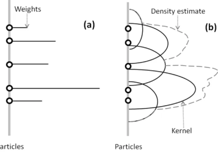
Fig. 1. The concept of discrete and continuous approximation of particle density: (a)weighted empirical measure, and(b) regular-ized measure by kernel. Adapted from Musso et al. (2001).
In this paper, we apply particle filters for a distributed hydrologic model in support of short-term hydrologic fore-casting. A lagged particle filtering approach is proposed to consider different response times of internal states in a distributed hydrologic model. The regularized particle fil-ter with the Markov chain Monte Carlo (MCMC) move step is also adopted to improve sample diversity under the lagged filtering approach. A process-based distributed hydrologic model, WEP (Jia and Tamai, 1998; Jia et al., 2001, 2009), is implemented for sequential data assimilation through state updating of internal hydrologic variables. Particle filtering is parallelized and implemented in the multi-core computing environment via an open message passing interface (MPI).
The paper is organized thus: Sect. 2 outlines the Bayesian filtering theory and particle filters. In Sect. 3, a lagged filter-ing approach is introduced with an additional regularization step to reflect different responses of internal processes in se-quential data assimilation. Section 4 presents the case study results, demonstrating the applicability of the proposed par-ticle filtering approach. The lagged regularized parpar-ticle filter (LRPF) and the sequential importance resampling (SIR) par-ticle filter are evaluated for hindcasting of streamflow in the Katsura River catchment using the WEP model. Section 5 summarizes the results and conclusions.
2 Method of particle filters
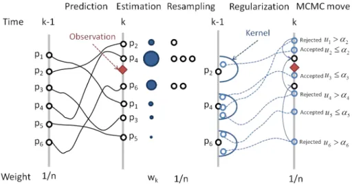
Fig. 2.A single cycle of a regularized particle filter.
Carlo methods can be found in Arulampalam et al. (2002) and Moradkhani et al. (2005a).
2.1 Bayesian filtering theory and basic particle filtering methods
To define the problem of the Bayesian filtering, consider a general dynamic state-space model, which is described as: xk = f (xk−1,θ,uk) +ωk ωk ∼ N (0,Wk) (1)
yk = h xk,θ′
+ νk vk ∼ N (0,Vk) (2)
wherexk∈
∑
=−
≈
=
⋅
>
on on
ℜ
n∫
=
∫
=
∫
<
∞
>
)
⋅
nx is then
x dimensional vector denoting the
system state at timek. The operatorf:
∑
=−
≈
=
⋅
>
on on
ℜ
n∫
=
∫
=
∫
<
∞
>
)
⋅
nx→
∑
=−
≈
=
⋅
>
on on
ℜ
n∫
=
∫
=
∫
<
∞
>
)
⋅
nxexpresses the system transition in response to the forcing data uk
(e.g. rainfall, weather data) and parametersθ.h:
∑
=−
≈
=
⋅
>
on on
ℜ
n∫
=
∫
=
∫
<
∞
>
)
⋅
nx→
∑
=−
≈
=
⋅
>
on on
ℜ
n∫
=
∫
=
∫
<
∞
>
)
⋅
ny express the measurement function, having parametersθ′.ωk
andνkrepresent the model error and the measurement error,
respectively, andWkandVk represent the covariance of the
error.
In the Bayesian recursive estimation, if the system and measurement models are non-linear and non-Gaussian, it is not possible to construct the posterior probability density function (PDF) of the current statexkgiven the measurement
y1:k={yi,i= 1, ...,k}analytically. When the analytic solu-tion is intractable, an optimal solusolu-tion can be approximated by SMC filters.
Sequential Monte Carlo (SMC) filters are a set of simulation-based methods that provide a flexible approach to computing posterior distribution without any assumptions being made about the nature of the distributions. The key idea of SMC filters is based on point mass (“particle”) repre-sentations of probability densities with associated weights: p xk|y1:k
≈
n
X
i=1
wikδxk −xik
(3)
wherexik andwki denote thei-th posterior state (“particle”) and its weight, respectively, andδ(·)denotes the Dirac delta function. Since it is usually impossible to sample from the true posterior PDF, an alternative is to sample from a pro-posal distribution, also called importance density, denoted by q(xk|yk). After several steps of computation, the recursive
weight updating can be derived as: wik ∝ wki−1 p yk|x
i k
p xik|xik−1
q xik|xik−1,yk . (4) The choice of importance density is one of the most criti-cal issues in the design of SMC methods. The most popular choice is the transitional prior:
qxik|xik−1,yk = pxik|xik−1. (5) By substituting Eq. (5) into Eq. (4), the weight updating becomes:
wik ∝ wki−1pyk|xik. (6) The sequential importance sampling (SIS) algorithm shown above is a Monte Carlo filter that forms the basis for most SMC filters. A common problem with the SIS algorithm is the degeneracy phenomenon, in which after a few iterations, all but one particle will have negligible weight. A suitable measure of the degeneracy is the effective sample sizeneff estimated as (Kong et al., 1994):
neff = 1
Pn i=1 wik
2. (7)
If the weights is uniform (i.e.wik= 1/nfori= 1, ...,n), then neff=n. If all but one particle have 0 weight, thenneff= 1. The ratio of the effective particle numbernratiois estimated as follows:
nratio = neff
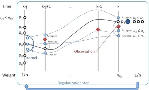
Fig. 3.Particle traces in the regularization step under the lagged filtering approach.
The maximum ofnratio is 1 when the weights are uniform. Small nratio indicates a severe degeneracy and vice versa. nratiois used as an indicator of degeneracy in this study be-cause it can be used easily regardless of the particle number. The degeneracy phenomenon can be reduced by perform-ing the resamplperform-ing step whenever a significant degeneracy is observed. Thus, the SIR particle filter is derived from the SIS algorithm by performing the resampling step at every time in-dex. The idea of resampling is simply that particles with very low weights are abandoned, while multiple copies of parti-cles are kept with the uniformly weighted measure{xik, n−1}, which still approximates the posterior PDF,p(xk|y1:k)(van
Leeuwen, 2009).
Resampling is one of the key issues in the SMC filters, and various resampling approaches have been introduced in the literature, such as multinomial resampling, residual resam-pling, stratified resamresam-pling, and systematic resampling. A comparative analysis and review of resampling approaches can be found in Douc et al. (2005) and van Leeuwen (2009). Systematic resampling, also known as stochastic universal sampling, is often preferred due to its computational simplic-ity and good empirical performance. It has also been shown that systematic resampling has the lowest sampling noise (Kitagawa, 1996). Hence, we use systematic resampling for all particle filtering cases in this study. It is worth noting that there are several choices in resampling methods, and the proper method may be different, depending on the character-istics of hydrologic models. See Weert and El Serafy (2006), Rings et al. (2010), and Salamon and Feyen (2009) for resid-ual resampling; see also Salamon and Feyen (2010) and Moradkhani et al. (2005a) for systematic resampling. Al-though the SIR method has the advantage that the importance weights are easily evaluated, because resampling is applied
at every iteration, this filter may lead to a sudden loss of di-versity in particles and is sensitive to outliers (Ristic et al., 2004).
2.2 Regularized particle filter
Assign the particle weights uniformly
n wi
t j k−+(−1)=1/
Propagate the n model states forward in time through model operator f(.)
Predict the system output through the operator h(.)
Update the particle weights Estimate the likelihood
Forecast based on updated particles t < j+1
t = t + 1
t j k t j k i t j k i t j
k f x u
x−+ = ( −+(−1), −+)+ω−+
) , 0 (
~ k jt
t j
k−+ N W−+
ω t j k i t j k i t j k hx
y−+ = ( −+)+ν −+ νk−j+t~N(0,Vk−j+t)
∑
= −+ −+ −+ + − + − + − + − − − = n i t j k i t j k t j k t j k i t j k t j k i t j k V x h y p V x h y p w 1 ] | ) ( [ ] | ) ( [ ] | ) ([ k jt
i t j k t j
k hx V
y
p −+ − −+ −+
Calculate the empirical covariance matrix Lk of
Compute Dk such that
Calculate lagged weight and likelihood
i i
k lag w
wˆ =
{ }
ˆ ] [ SUM 1 n i i lag w temp= =i lag i
lag temp w
w = −1~
Draw from the Epanechnikov/Gaussian kernel
k T k
kD L
D =
{
}
n i i lag i k w x 1 , = K i ~ ε i k opt i t j k i t jk x h D
x−+(−1)*= −+(−1)+ ε
i i k lag L L = Generate
Calculate acceptance probability
Accept if ] 1 , 0 [ ~U u = i i lag lag L L * , 1 min α * i k
x u≤α
Implement the resampling Yes
No
Yes
No
Next time step
neff < nthr or . thr k k k y y x h y − ( )|< |
max
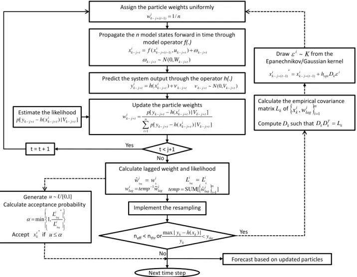
Fig. 4.The flow diagram of regularized particle filter with MCMC move step in the lagged filtering approach.
In RPF, posterior particles are drawn from the approximation
p xk|y1:k
≈
n
X
i=1 wikKh
xk −xik
(9) where
Kh(x) =
1 hnx K
x
h
(10) is the rescaled kernel densityK(·),h >0 is the bandwidth, andnx is the dimension of the state vectorx. The kernel
density is a symmetric probability density function on
∑
=−
≈
=
⋅
>
on on
ℜ
n∫
=
∫
=
∫
<
∞
>
)
⋅
nx, such that
K > 0
Z
K(x)dx =1
Z
xK(x)dx = 0 (11)
Z
kxk2K(x)dx < ∞.
The kernel K(·)and bandwidthh are chosen to minimise the mean integrated square error (MISE) between the true
posterior density and the corresponding regularized weighted empirical measure in Eq. (9), which is defined as
MISE(p)ˆ = E
Z
ˆ
p xk
y1:k
−p xk
y1:k
2
dxk
(12) wherep(ˆ ·|·)denotes the approximation top(xk
y1:k) given
by the right-hand side of Eq. (9). In the special case of equally weighted samples, wi= 1/n for i= 1, ...,n, the op-timal choice of the kernel is the Epanechnikov kernel,
Kopt =
nx+2
2cnx 1−kxk 2
if kxk < 1
0 otherwise
(13)
wherecnxis the volume of the unit sphere of
∑
=−
≈
=
⋅
>
on on
ℜ
n∫
=
∫
=
∫
<
∞
>
)
⋅
nx. It is worth noting that the use of kernel approximation becomes increas-ingly less appropriate asnx(dimensionality of the state)
Table 1.Simulation periods and observed flow.
Simulation period Max. observed flow Data availability at each location
at Katsura (m3s−1) Katsura Kameoka
1 Jun–31 Jul 2007 336.9 O X
1 Aug–30 Oct 2004 2276.7 O O
1 Jun–31 Aug 2003 361.6 O O
Fig. 5.The Katsura River catchment.
hopt =A ·n−nx1+4 with (14)
A = h8c−n1
x (nx +4) 2
√
πnxi 1 nx+4
.
RPF differs from SIR only in additional regularization steps when sample impoverishment happens. The key step is
xik∗ = xik +hoptDkεi (15)
wherexik∗ is a new particle generated from kernel density, Dk is estimated fromSk, which is the empirical covariance
matrix such thatDkDTk =Lk, andεi is the random noise from
the kernel. Note that the calculation of the empirical covari-ance matrixLk is carried out prior to the resampling and is
therefore a function of both thexik andwik. The theoretical disadvantage of RPF is that its samples are no longer guaran-teed to asymptotically approximate those from the posterior. This can be mitigated by including the Markov chain Monte Carlo (MCMC) move step (Gilks and Berzuini, 2001) based on the Metropolis-Hastings algorithm (Robert and Casella,
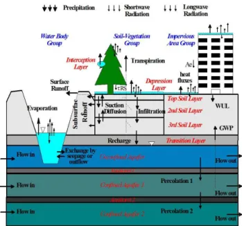
Fig. 6. A schematic view of WEP model structure. Adapted from Jia et al. (2009).
1999). The key idea is that a resampled particle is moved to a new state, according to Eq. (15), only ifu≤α, where u∼U[0, 1] andαis the acceptance probability. Otherwise, the move is rejected.
α =
min
(
1, p
yk|xi∗ k
pyk|xik
)
if p yk|xik
6= 0
1 otherwise
. (16)
In Eq. (16),αbecomes 1.0 when the likelihood of new par-ticle is greater than that of the previous parpar-ticle. That means that the MCMC move step contributes to screening bad par-ticles in the regularization step, thus ensuring that parpar-ticles asymptotically approximate samples from the posterior.
in the MCMC move step. Although this approach is fre-quently found to improve performance with a less rigorous deviation, RPF has not been introduced in hydrologic data assimilation.
3 Particle filter with lag time approach
Many hydrological processes operate – in response to precip-itation – at similar length scales, but the time scales are de-layed (Bloschl and Sivapalan, 1995). In a distributed hydro-logic model, there are many types of state variables, and each variable interacts with others based on different time scales. For example, in catchment modelling, internal state variables may refer to two-dimensional distribution of soil moisture content, evapotranspiration, and overland flow; and an ob-servable state may refer to streamflow flux at the monitoring sites. There is a time lag until the changes of soil moisture distribution affect infiltration and sub-surface/surface runoff processes and generated runoff is routed as streamflow into the measurement site. Hydrologic components in a hydro-logic model have usually different time scales, which need to be considered in the data assimilation process.
As stated by Salamon and Feyen (2010), this response time is usually greater than the high-frequency discharge mea-surements. One simple approach is to use delayed updat-ing, which utilizes longer time intervals before updating state variables. However, delayed updating leads to omitting large quantities of measurement information, and a fixed delay as-sumption may result in inappropriate estimation, because a response time always changes, depending on the current spa-tial distributions of the state and forcing variables. Further-more, when system behaviour is relatively fast (e.g. hourly based hydrologic or hydraulic modelling cases), delayed up-dating may lead to missing proper timing of assimilation. That can make it hard to implement sequential data assim-ilation techniques into hydrologic modelling. Thus, we pro-pose a new lagged particle filtering approach based on the regularized particle filter, not only for considering different catchment responses, but also for using whole measurement information for data assimilation.
Figure 3 shows an example of a newly proposed lagged particle filtering approach with RPF. Here,k is the current time step, andj is the lag time required for responses of internal state variables to be transmitted into the observ-able variobserv-ables. Note that it is better to set the lag time j large enough to cover plausible ranges because the system response is time-variant.
The assimilation window of the lagged filtering is defined fromk−j toktime step. The procedure of the lagged fil-tering is as follows: (1) to have prediction at the time stepk, simulation starts from the time stepk−j. (2) When particles arrive at the current timek, the lagged weights are estimated according to the measurement. (3) Resampling is executed according to the lagged weights. Note that state variables
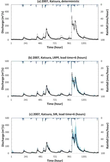
Fig. 7.Observed versus 6-h-lead forecasts at the Katsura station via LRPF and SIR (1 June–31 July 2007):(a)a deterministic modelling case;(b)LRPF; and(c)SIR. The blue line and area represent the mean value and 90 % confidential intervals, respectively. A gray dashed line represents a deterministic modelling case. The black dots represent observed discharge.
stepk−j+ 1 should be stored and resampled according to lagged weights.
Lagged weight,wilag, and lagged likelihood,Lilag, can be calculated through various methods, including the aggrega-tion of the past weight. However, in this study, the weight and likelihood at the last time stepk(wki,Lik) are simply used as lagged weight and likelihood, respectively. Note that the use of weights without aggregation can show better results in cases of short-term forecasting.
Figure 4 summarises one cycle of the algorithm of RPF with the Markov chain Monte Carlo (MCMC) move step un-der the lagged filtering approach. The procedure connected with the dashed line means the regularization step. It is worth mentioning that the regularization step can be executed not just in the sample impoverishment, but also in the parti-cle collapse case, which means all partiparti-cles have negligible weights that fall outside the measurement PDF. In this case, the regularization step is used effectively for re-initialization of the particle system.
4 Implementation
4.1 Study area
The SMC methods are applied to the Katsura River catch-ment (Fig. 5) to show the applicability of the proposed par-ticle filtering approach. This catchment is located in Kyoto, Japan, and covers an area of 1100 km2(887 km2at the Kat-sura station) (see Fig. 5). Topography in the catchment is characterized by a mountainous upstream in the north and a flatter plain in the south. The elevation in the catchment ranges from 4 to 1158 m, with an average of about 325 m. The land use consists of forest (76.7 %), agricultural area (9.3 %), residential area (7.5 %), water body (2.0 %), pub-lic area (2.7 %), vacant land (1.2 %), and road (0.6 %), re-spectively. There are 13 rainfall observation stations, 1 me-teorological observation station, and 4 river flow observa-tion staobserva-tions. Annual precipitaobserva-tion and temperature are about 1422 mm and 16.2◦ in Kyoto city (2001∼2010). Precip-itation is concentrated in the summer season from May to September. The Hiyoshi dam is located upstream. The con-trolled outflow record from the dam reservoir is given as inflow to the hydrologic model, and the model simulates rainfall-runoff processes for the downstream of the dam. 4.2 Hydrological model and particle filtering
The hydrologic model used is the water and energy transfer processes (WEP) model, which was developed for simulating spatially variable water and energy processes in catchments with complex land covers (Jia and Tamai, 1998; Jia et al., 2001). State variables of WEP include soil moisture content, surface runoff, groundwater tables, discharge and water stage in rivers, heat flux components, etc. (Fig. 6). The spatial cal-culation unit of the WEP model is a square or rectangular
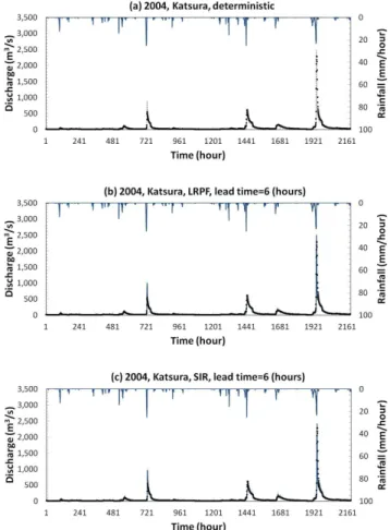
Fig. 8. Observed versus 6-h-lead forecasts at the Katsura station via LRPF and SIR (1 August–30 October 2004):(a)a deterministic modelling case;(b)LRPF; and(c)SIR. The blue line and area rep-resent the mean value and 90 % confidential intervals, respectively. A gray dashed line represents a deterministic modelling case. The black dots represent observed discharge.
grid. Runoff routing on slopes and in rivers is carried out by applying a one-dimensional kinematical wave approach from upstream to downstream. The WEP model has been applied in several watersheds in Japan, Korea, and China with differ-ent climate and geographic conditions (Jia et al., 2001, 2009; Kim et al., 2005; Qin et al., 2008).
The model setup uses 250 m grid resolution and an hourly time step. We use hourly observed rainfall from 13 obser-vation stations organized by the Ministry of Land, Infras-tructure, Transport and Tourism in Japan (http://www1.river. go.jp/) and hourly observed meteorological data including air temperature, relative humidity, wind speed, and dura-tion of sunlight from the Kyoto stadura-tion, which is organized by Japan Meteorological Agency (http://www.jma.go.jp/jma/ index.html). The nearest neighbour interpolation method is used for representation of spatial distribution of rainfall.
and Agriculture Organization of the United Nations (http: //www.fao.org/nr/land/soils/en/). Physical property of soil is derived from soil texture information using the ROSETTA model (Schaap et al., 2001). However, the saturated hy-draulic conductivity of several soils is roughly adjusted for the data period of 2007, since soil property estimated from large-scale soil maps varies greatly. For other parameters re-lated to aquifers and vegetation, we apply parameter ranges from the earlier studies mentioned above. No flux bound-ary condition is specified at the catchment boundbound-ary for the groundwater flow. Artifical water use is approximately es-timated as 3 m3s−1and subtracted directly from simulated discharge at the Katsura station.
Ensemble simulation of 192 particles is conducted on a multi-processing computer (96 cores in the supercomputing system of Kyoto University) via parallel-computing tech-niques of open message passing interface (MPI) (http://www. open-mpi.org/). The parallel programming code is writ-ten using a single-program multiple-data (SPMD) approach, which means the same modelling procedure with different state variables. A master process aggregates particle statis-tics and controls resampling/regularization steps. Message passing commands of MPI is used effectively to transfer spa-tially distributed state variables from one particle to another in the resampling step.
4.3 Process and measurement error models
Particle filters perform suboptimal estimation of the system states by considering the uncertainty in both the measure-ment and modelling systems. Therefore, the choice of the er-ror models is crucial to obtaining a better estimation (Weert and El Serafy, 2006). Another important point is to choosing hidden state variables for filtering. Since there are numer-ous state variables in a distributed hydrologic model, it is not practical to consider the uncertainty of all state variables with a limited number of particles. Therefore, it is necessary to choose a limited number of state variables, which process error of the modelling system is aggregated in, and is easily updated by observable variables. In this study, we select soil moisture content and overland flow in each grid as hidden state variables and streamflows at the Katsura station as an observable variable for data assimilation. Global multipliers are introduced to perturb state variables stochastically and ef-fectively. In the case of soil moisture content, the total soil moisture depth at the previous time stepSk−1is aggregated for three soil layers within the catchment as:
Sk−1 = 3
X
l=1
m
X
j=1
θjl djl (17)
where θjl and djl are the volumetric soil moisture content (m3m−3) and the soil depth (m) in each layer, andlandm represent the number of soil layers and the total number of grids within the catchment, respectively. Then, process noise
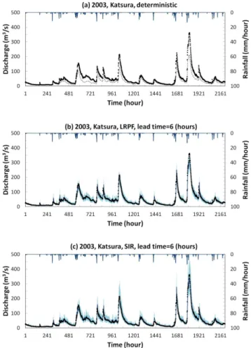
Fig. 9. Observed versus 6-h-lead forecasts at the Katsura station via LRPF and SIR (1 June–31 August 2003): (a)a deterministic modelling case;(b)LRPF; and(c)SIR. The blue line and area rep-resent the mean value and 90 % confidential intervals, respectively. A gray dashed line represents a deterministic modelling case. The black dots represent observed discharge.
of the soil moisture contentwsoilkis added to the aggregated state variableSk−1as:
ˆ
Sk = Sk−1 +wsoilk. (18) wsoilk is assumed as Gaussian distributionN(0,σsoilk2 ) having a heteroscedastic standard deviation as:
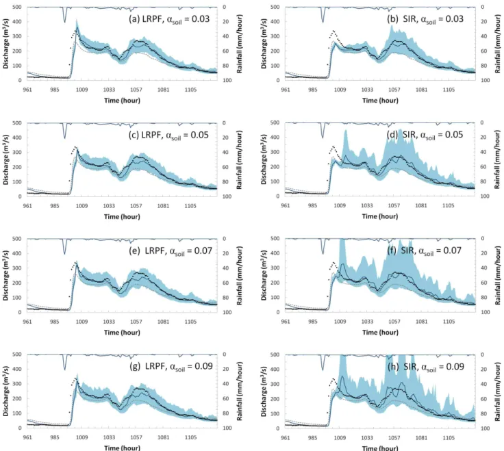
Fig. 10. Observed versus 6-h-lead forecasts at the Katsura station via LRPF and SIR for varying parameter values of the process error variance,αsoil(11 to 17 July 2007). The blue line and area represent the mean value and 90 % confidential intervals, respectively. A gray
dashed line represents a deterministic modelling case. The black dots represent observed discharge.
the perturbed states of soil moistureθˆjl are calculated using multiplicative factorγsas follows:
γs =
ˆ
Sk
Sk−1
(20)
ˆ
θjl = γsθjl. (21)
In the above equations, if perturbed soil moisture at each grid and layer,θˆjl, becomes greater or smaller than the physical limitation, θˆjl is adjusted at its maximum (i.e. porosity) or minimum (i.e. wilting point). It is also worth noting that
Fig. 11. Observed versus forecasts of varying lead times at the Katsura station via LRPF and SIR withαsoil of 0.05 (11 to 17 July 2007):(a)the lagged regularization particle filter (LRPF); and(b)the SIR particle filter. The blue lines represent forecasts of varying lead times. A gray dashed line represents a deterministic modelling case. The black dots represent observed discharge.
The perturbation of overland flow is also applied in a mul-tiplicative way as:
ˆ
qovj = 1 +wovkqovj (22) whereqovj andqˆovj are overland flow with and without pro-cess noisewovk, respectively, which is assumed as a Gaussian distributionN (0, σovk2 ). The standard deviation of overland flow noiseσovk is parameterized as follows:
σovk = cov10αovexp(−ysimk−1/βov) (23) whereαovandβovare adaptable parameters with settings of
−10 and 5 m3s−1, respectively, as obtained from sensitivity analysis. ysimk−1is the simulated discharge of data assimila-tion at the previous time step. covis the constant coefficent. The value ofcovis estimated through the sensitivity analysis and set as 0.02 for the whole simulation. This formulation was originally proposed by Seo et al. (2009) to enhance the forecast in periods of low flow. Equation (23) specifies pro-gressively smaller uncertainty if the simulated flow falls be-low the threshold,βov(m3s−1). We adopt this error formu-lation because an error of overland flow routing is expected to decline in low flow periods.
The measurement error of the discharge is assumed as a Gaussian distributionN (0, σobs2
k)similar to previous studies (Georgakakos, 1986; Weert and El Serafy, 2006; Salamon
Fig. 12.Nash-Sutcliffe model efficiency for varying parameter val-ues of the process error variance,αsoil. The red lines represent the lagged regularized particle filter. The dashed lines represent the SIR particle filter. A dotted line represents a deterministic modelling case.
and Feyen, 2010). The standard deviation of the measure-ment error is chosen as:
σobsk = αobsyk +βobs. (24) In Eq. (24),αobsis set as 0.1, which means 10 % of the mea-surement error, and the constant coefficientβobsis applied as 5 m3s−1to consider uncertainty in periods of low flow such as artificial water use and dam reservoir control. The uncer-tainty of forcing data is not considered in this study to make it easy to evaluate the difference of each particle filter. Fif-teen percent of perturbation from the uniform distribution is applied for the initial soil moisture condition.
4.4 Results and discussion
Fig. 13.Nash-Sutcliffe model efficiency for varying parameter values of the process error variance,αsoil. The red lines represent the lagged
regularized particle filter. The dashed lines represent the SIR particle filter. A dotted line represents a deterministic modelling case.
Simulation periods and observation are shown in Table 1. Hourly observed discharges at the Katsura station are used for the data assimilation, and observation at the Kameoka station is used for comparison. A five-day warm-up period is added before the data assimilation starts.
Deterministic simulation results and 6-h-lead forecasts of each particle filter at the Katsura station for the years 2007, 2004, and 2003 are shown in Figs. 7, 8, and 9, respectively. The lag time of 8 h is applied in LRPF. The applied val-ues ofαsoil are 0.05 for 2007 and 0.03 for 2004 and 2003. The forecasted streamflow via two particle filters shown in Figs. 7 and 9 indicates good conformity between observation and simulation, while the deterministic modelling shows sig-nificant underestimation, especially in the high flood regime. Ninety percent of confidential intervals of SIR are larger than those of LRPF, although the same error assumption is used. Compared with results of other years, the differences of con-fidential intervals between two filters are small in the year of 2004, shown in Fig. 8, since the deterministic modelling results show better agreement with observation, relatively. Elapsed simulation time for the year of 2007 is about 11 h in SIR and 16 h in LRPF for a 2-month period simulation with 24-h-lead forecast at every time step, respectively.
Various ranges of proccess noise,αsoil, are simulated for each particle filter to assess the effects of process noise on the forecast. The mean and 90 % confidential intervals of 6-h-lead forecasts for varying parameter value ofαsoil are illustrated in Fig. 10. In the case of SIR, confidential intervals of forecast widen rapidly, and the ensemble mean becomes unstable when the value ofαsoilincreases. On the other hand, those of LRPF show stable results regardless of the process noise.
Table 2.Statistics of streamflow forecasts with varying lead times (αsoil= 0.03).
Year Method Lead time (hour)
1 3 6 12 24
NSE RMSE COR NSE RMSE COR NSE RMSE COR NSE RMSE COR NSE RMSE COR 2007 DET 0.87 16.7 0.96 0.87 16.7 0.96 0.87 16.7 0.96 0.87 16.7 0.96 0.87 16.7 0.96 LRPF 0.98 7.9 0.99 0.95 11.5 0.98 0.93 13.6 0.97 0.91 16.1 0.95 0.88 18.3 0.94 SIR 0.96 10.1 0.98 0.95 12.2 0.97 0.93 13.7 0.97 0.91 15.6 0.96 0.88 18.2 0.95 2004 DET 0.84 59.9 0.93 0.84 59.9 0.93 0.84 59.9 0.93 0.84 59.9 0.93 0.84 59.9 0.93 LRPF 0.89 48.1 0.95 0.85 57.5 0.92 0.86 55.4 0.93 0.84 58.8 0.93 0.83 61.4 0.92 SIR 0.87 53.2 0.93 0.85 56.8 0.92 0.85 56.9 0.93 0.84 59.7 0.92 0.83 61.1 0.92 2003 DET 0.70 26.9 0.98 0.70 26.9 0.98 0.70 26.9 0.98 0.70 26.9 0.98 0.70 26.9 0.98 LRPF 0.99 4.4 1.00 0.98 6.7 0.99 0.96 9.4 0.98 0.93 12.6 0.97 0.87 17.6 0.96 SIR 0.99 4.5 1.00 0.98 6.5 0.99 0.97 9.0 0.98 0.94 12.1 0.97 0.89 16.6 0.96
while the recovery of particle diversity needs more time steps in the case of SIR.
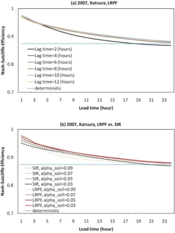
Figure 12 shows the sensitivity of the lag time of LRPF and process noise parameter,αsoil, for each particle filter are estimated for varying lead times in the year of 2007 using Nash-Sutcliffe efficiency calculated as:
E = 1 −
PT
k=1 yk −ysimk
2 PT
k=1(yk − ¯y)2
(25)
whereyis observation,y¯is the mean of observation,ysimkis the forecasted streamflow at the measurement site, andT is the total number of time steps.
When the lag time is larger than 4 h, the difference of Nash-Sutcliffe efficiency (NSE) for varying lead times be-comes negligible, as shown in Fig. 12a. Eight hours of the lag time are applied to the other simulations by LRPF. NSE scores for varying lead times show different behaviours for each particle filter (Fig. 12b). While NSE of LRPF shows a consistent behaviour regardless of error assumption, with all the red lines overlapping along the lead time, that of SIR changes according to the values of αsoil. Overall, LRPF shows improved NSE for any range of αsoil. NSE shows rather significant differences between the two particle filters when plotted for the high flows (not shown).
Figure 13 shows NSE of each particle filter for varying lead times in the years 2004 and 2003. Overall, LRPF fore-casts show less variation compared to SIR forefore-casts, except the forecast of 2003 at Kameoka. Similarly to the year 2007 (Fig. 12b), NSE scores of SIR in 2004 and 2003 drop sharply when the process errorαsoilincreases. Although NSE scores of LRPF show less change than does SIR, NSE differences of LRPF of 2003 increase according to the lead time. Rela-tively excessive perturbation in the regularization step for the smoothly varied flood events may be one potential reason. However, differences of NSE appear to be neglible within 8-h lead times. T8-he forecasts at Kameoka s8-how reduced NSE
scores in both particle filters. In the case of 2004, LRPF shows better forecasts within 4-h lead times, while SIR out-performs for other lead times in 2004 and 2003. Since the H-Q relationship of Kameoka is made with limited data, the Kameoka station appears to have larger uncertainty than does Katsura. Due to the lack of data, more extensive comparison is beyond the scope of this study. Nevertheless, we can ob-serve that the statistical stability of LRPF is superior to that of SIR in terms of confidention intervals and accuracy for un-certain process noise,αsoil(not shown), similar to the results of 2007 (Fig. 10).
Table 2 shows statistics of streamflow forecasts with vary-ing lead times at Katsura includvary-ing NSE, root mean square error (RMSE) and correlation coefficient (COR) for a given process noise (αsoil= 0.03). Statistics shown in Table 2 indi-cate that LRPF is somewhat better than SIR especially in the years 2007 and 2004. The improvement by LRPF over SIR is larger for shorter lead times and the high flows (not shown). COR shows high values for both cases in overall periods. It is worth noting that SIR has different optimum values of pro-cess noise for data periods, and thus it shows large variation of statistics depending on the process noise (not shown) as the patterns shown in Figs. 12 and 13.
5 Conclusions
Two particle filters showed significantly improved fore-casts compared to deterministic modelling cases in different simulation periods. Various ranges of process noise related to soil moisture were simulated for varying lead times. While SIR has different values of optimal process noise and shows sensitive variation of confidential intervals according to the process noise, LRPF shows consistent forecasts regardless of the process noise assumption. Due to the preservation of particle diversity by the kernel, LRPF showed enhanced forecasts, especially when the discharge changed sharply in a short time (the year 2007) and flood peak was high (the year 2004). However, the relatively large perturbation by the kernel could produce negative effects when the flood peak was relatively small and the hydrograph varied smoothly (the year 2003).
SMC methods have significant potential for high non-linearity problems, especially for process-based distributed models in hydrologic investigation. However, the computa-tional cost and marginal adequacy of SMC methods for dis-tributed modelling have been bottlenecks to their practical implementation. As shown in this study, a particle filtering process can be effectively parallelized and implemented in the multi-core computing environment via MPI library. The LRPF is expected to be used as one of the frameworks for se-quential data assimilation of process-based distributed mod-elling. The main benefits of LRPF are the improved forecasts for rapidly varied high floods and the stability of confidential intervals for uncertainty of process noise. More extended im-plementation for multi-site forecasting and effective sequen-tial estimation of model parameters remain open problems, indeed.
Acknowledgements. We thank S. Ushijima at the Academic Center for Computing and Media Studies, Kyoto University, for his guidance in using the super computer system and MPI.
Edited by: Y. Liu
References
Arulampalam, M. S., Maskell, S., Gordon, N., and Clapp, T.: A tutorial on particle filters for online nonlinear/non-Gaussian Bayesian tracking, IEEE T. Signal Process., 50, 174–188, 2002. Bloschl, G. and Sivapalan, M.: Scale issues in hydrological
mod-elling: a review, Hydrol. Process., 9, 251–290, 1995.
Clark, M. P., Rupp, D. E., Woods, R. A., Zheng, X., Ibbitt, R. P., Slater, A. G., Schmidt, J., and Uddstrom, M. J.: Hydrological data assimilation with the ensemble Kalman filter: use of stream-flow observations to update states in a distributed hydrological model, Adv. Water Resour., 31, 1309–1324, 2008.
Douc, R., Cappe, O., and Moulines, E.: Comparison of resampling schemes for particle filtering, in: Proceedings of the 4th Interna-tional Symposium on Image and Signal Processing, 64–49, 2005. Evensen, G.: Sequential data assimilation with a nonlinear quasi-geostrophic model using Monte Carlo methods to forecast error statistics, J. Geophys. Res., 99, 10143–10162, 1994.
Evensen, G.: Data Assimilation: The ensemble Kalman Filter, Springer, 2009.
Georgakakos, K. P.: A generalized stochastic hydrometeorological model for flood and flash-flood forecasting, Water Resour. Res., 22, 2096–2106, 1986.
Gilks, W. R. and Berzuini, C.: Following a moving target – Monte Carlo inference for dynamic Baysian models, J. Roy. Stat. Soc. B, 63, 127–146, 2001.
Gordon, N. J., Salmond, D. J., and Smith, A. F. M.: Novel approach to nonlinear/non-Gaussian Bayesian state estimation, Proc. Inst. Electr. Eng., 140, 107–113, 1993.
Jia, Y. and Tamai, N.: Integrated analysis of water and heat bal-ance in Tokyo metropolis with a distributed model, J. Jpn. Soc. Hydrol. Water Res., 11, 150–163, 1998.
Jia, Y., Ni, G., Kawahara, Y., and Suetsugi, T.: Development of WEP model and its application to an urban watershed, Hydrol. Process., 15, 2175–2194, 2001.
Jia, Y., Ding, X., Qin, C., and Wang, H.: Distributed modeling of landsurface water and energy budgets in the inland Heihe river basin of China, Hydrol. Earth Syst. Sci., 13, 1849–1866, doi:10.5194/hess-13-1849-2009, 2009.
Johansen, A. M.: SMCTC: sequential Monte Carlo in C++, J. Stat. Softw., 30, 1–41, 2009.
Karssenberg, D., Schmitz, O., Salamon, P., de Jong, K., and Bierkens, M. F. P.: A software framework for construction of process-based stochastic spatio-temporal models and data assim-ilation, Environ. Model. Softw., 25, 489–502, 2010.
Kim, H., Noh, S., Jang, C., Kim, D., and Hong, I.: Monitoring and analysis of hydrological cycle of the Cheonggyecheon watershed in Seoul, Korea, in: Proc. of International Conference on Sim-ulation and Modeling, Nakornpathom, Thailand, 2005, C4–03, 2005.
Kim, S., Tachikawa, Y., and Takara, K.: Applying a recursive up-date algorithm to a distributed hydrologic model, J. Hydrol. Eng., 336–344, 2007.
Kitagawa, G.: Monte-Carlo filter and smoother for non-Gaussin non-linear state-space models, J. Comput. Graph. Stat., 5, 1–25, 1996.
Kitanidis, P. K. and Bras, R. L.: Real-time forecasting with a con-ceptual hydrologic model 2. applications and results, Water Re-sour. Res., 16, 1034–1044, 1980.
Kong, A., Liu, J. S., and Wong, W. H.: Sequential imputations and Bayesian missing data problems, J. Am. Stat. Assoc., 89, 278– 288, 1994.
Leisenring, M. and Moradkhani, H.: Snow water equivalent pre-diction using Bayesian data assimilation methods, Stoch. Envi-ron. Res. Risk A., 25, 253–270, doi:10.1007/s00477-010-0445-5, 2010.
Liu, Y. and Gupta, H. V.: Uncertainty in hydrologic modeling: to-ward an integrated data assimilation framework, Water Resour. Res., 43, W07401, doi:10.1029/2006WR005756, 2007. Montanari, M., Hostache, R., Matgen, P., Schumann, G.,
Pfis-ter, L., and Hoffmann, L.: Calibration and sequential updating of a coupled hydrologic-hydraulic model using remote sensing-derived water stages, Hydrol. Earth Syst. Sci., 13, 367–380, doi:10.5194/hess-13-367-2009, 2009.
Moradkhani, H., Hsu, K.-L., Gupta, H., and Sorooshian, S.: Un-certainty assessment of hydrologic model states and parameters: sequential data assimilation using the particle filter, Water Re-sour. Res., 41, W05012, doi:10.1029/2004WR003604, 2005a. Moradkhani, H., Sorooshian, S., Gupta, H. V., and Houser, P. R.:
Dual state-parameter estimation of hydrological models using ensemble Kalman filter, Adv. Water Res., 28, 135–147, 2005b. Musso, C., Oudjane, N., and Le Gland, F.: Improving regularized
particle filters, in: Sequential Monte Carlo in Practice, edited by: Doucet, A., de Freitas, N., and Gordon, N., Springer-Verlag, New York, 247–271, 2001.
Noh, S. J., Tachikawa, Y., Shiiba, M., and Kim, S.: Dual state-parameter updating scheme on a conceptual hydrologic model using sequential Monte Carlo filters, Annual Journal of Hy-draulic Engineering, JSCE, 55, 1–6, 2011.
Qin, C., Jia, Y., Su, Z., Zhou, Z., Qiu, Y., and Suhui, S.: Integrating remote sensing information into a distributed hy-drological model for improving water budget predictions in largescale basins through data assimilation, Sensors, 8, 4441– 4465, doi:10.3390/s8074441, 2008.
Qin, J., Liang, S., Yang, K., Kaihotsu, I., Liu, R., and Koike, T.: Simultaneous estimation of both soil moisture and model parameters using particle filtering method through the assim-ilation of microwave signal, J. Geophy. Res., 114, D15103, doi:10.1029/2008JD011358, 2009.
Reichle, R. H., McLaughlin, D. B., and Entekhabi, D.: Variational data assimilation of microwave radiobrightness observations for land surface hydrology applications, IEEE T. Geosci. Remote, 39, 1708–1718, 2001.
Rings, J., Huisman, J. A., and Vereecken, H.: Coupled hydrogeo-physical parameter estimation using a sequential Bayesian ap-proach, Hydrol. Earth Syst. Sci., 14, 545–556, doi:10.5194/hess-14-545-2010, 2010.
Ristic, B., Arulampalam, S., and Gordon, N.: Beyond the Kalman Filter: Particle Filters for Tracking Applications, Artech House, 2004.
Robert, C. P. and Casella, G.: Monte Carlo Statistical Methods, Springer, New York, 1999.
Salamon, P. and Feyen, L.: Assessing parameter, precipitation, and predictive uncertainty in a distributed hydrological model using sequential data assimilation with the particle filter, J. Hydrol., 376, 428–442, 2009.
Salamon, P. and Feyen, L.: Disentangling uncertainties in dis-tributed hydrological modeling using multiplicative error mod-els and sequential data assimilation, Water Resour. Res., 46, W12501, doi:10.1029/2009WR009022, 2010.
Schaap, M. G., Leij, F. J., and van Genuchten, M. T.: ROSETTA: a computer program for estimating soil hydraulic parameters with hierarchical pedotransfer functions, J. Hydrol., 251, 163–176, 2001.
Seo, D.-J., Koren, V., and Cajina, N.: Real-time variational assim-ilation of hydrologic and hydrometeorological data into oper-ational hydrologic forecasting, J. Hydrometeorol., 4, 627–641, 2003.
Seo, D.-J., Cajina, L., Corby, R., and Howieson, T.: Automatic state updating for operational streamflow forecasting via variational data assimilation, J. Hydrol., 367, 255–275, 2009.
Smith, P. J., Beven, K. J., and Tawn, J. A.: Detection of structural inadequacy in process-based hydrological models: A particle-filtering approach, Water Resour. Res., 44, W01410, doi:10.1029/2006WR005205, 2008.
van Delft, G., El Serafy, G. Y., and Heemink, A. W.: The ensemble particle filter (EnPF) in rainfall-runoff models, Sotch. Environ. Risk A., 23, 1203–1211, 2009.
van Leeuwen, P. J.: Particle filtering in geophysical systems, Mon. Weather Rev., 137, 4089–4114, 2009.
Vrugt, J. A., Gupta, H. V., Nuallain, B. O., and Bouten, W.: Real-time data assimilation for operational ensemble streamflow fore-casting, J. Hydrolmeteorol., 7, 548–565, 2006.
Weert, A. H. and El Serafy, G. Y. H.: Particle filtering and ensem-ble Kalman filtering for state updating with hydrological con-ceptual rainfall-runoff models, Water Resour. Res., 42, W09403, doi:10.1029/2005WR004093, 2006.