An assessment of climate state reconstructions obtained using particle filtering methods

(1)

CPD

9, 43–74, 2013

An assessment of climate state reconstructions

S. Dubinkina and H. Goosse

Title Page

Abstract Introduction

Conclusions References

Tables Figures

◭ ◮

Back Close

Full Screen / Esc

Printer-friendly Version Interactive Discussion

Discussion

P

a

per

|

Dis

cussion

P

a

per

|

Discussion

P

a

per

|

Discussio

n

P

a

per

|

Clim. Past Discuss., 9, 43–74, 2013 www.clim-past-discuss.net/9/43/2013/ doi:10.5194/cpd-9-43-2013

Climate of the Past Discussions

This discussion paper is/has been under review for the journal Climate of the Past (CP). Please refer to the corresponding final paper in CP if available.

An assessment of climate state

reconstructions obtained using particle

filtering methods

S. Dubinkina and H. Goosse

Earth and Life Institute, Georges Lemaˆıtre Centre for Earth and Climate Research, Universit ´e catholique de Louvain, P.O. Box L4.03.07, 1348 Louvain-la-Neuve, Belgium

Received: 12 December 2012 – Accepted: 18 December 2012 – Published: 3 January 2013

Correspondence to: S. Dubinkina (svetlana.dubinkina@uclouvain.be)

(2)

CPD

9, 43–74, 2013

Title Page

Tables Figures

◭ ◮

Back Close

Full Screen / Esc

Discussion

P

a

per

|

Dis

cussion

P

a

per

|

Discussion

P

a

per

|

Discussio

n

P

a

per

|

Abstract

In an idealized framework, we assess reconstructions of the climate state of the South-ern Hemisphere during the past 150 yr using the climate model of intermediate com-plexity LOVECLIM and three data-assimilation methods: a nudging, a particle filter with sequential importance resampling, and an extremely efficient particle filter. The meth-5

ods constrain the model by pseudo-observations of surface air temperature anoma-lies obtained from a twin experiment using the same model but different initial con-ditions. The net of the pseudo-observations is chosen to be either dense (when the pseudo-observations are given at every grid cell of the model) or sparse (when the pseudo-observations are given at the same locations as the dataset of instrumental 10

surface temperature records HADCRUT3). All three data-assimilation methods provide with good estimations of surface air temperature and of sea ice concentration, with the extremely efficient particle filter having the best performance. When reconstructing variables that are not directly linked to the pseudo-observations of surface air tem-perature as atmospheric circulation and sea surface salinity, the performance of the 15

particle filters is weaker but still satisfactory for many applications. Sea surface salinity reconstructed by the nudging, however, exhibits a patterns opposite to the pseudo-observations, which is due to a spurious impact of the nudging on the ocean mixing.

1 Introduction

Reliable reconstructions of the past climate states are essential for a comprehensive 20

understanding of the climate system, more accurate climate predictions and projec-tions. They enable to estimate the magnitude of the natural variability without an-thropogenic impact and to provide insights into the processes responsible for climate changes.

A new but highly appealing approach to reconstruct the past climate states is data 25

(3)

CPD

9, 43–74, 2013

Title Page

Tables Figures

◭ ◮

Back Close

Full Screen / Esc

Discussion

P

a

per

|

Dis

cussion

P

a

per

|

Discussion

P

a

per

|

Discussio

n

P

a

per

|

2012). The main purpose of data assimilation is to estimate the state of a system as accurately as possible incorporating all the available information: numerical modelling of the behaviour of the system, observations, and uncertainties of the model and of the observations (Talagrand, 1997). When choosing a data-assimilation method, the application to which it is applied should be kept in mind. For example, in meteorologi-5

cal applications data-assimilation methods like 4DVar (e.g. Courtier et al., 1994) or the ensemble Kalman filter (Evensen, 1994) are employed. These methods, however suc-cessful, are biased in the sense that they assume the Gaussian prior distribution. But the prior distribution can take any form because the system is nonlinear.

There exists an ensemble-based data-assimilation method that does not make such 10

an assumption. It is particle filtering. In particle filtering, the probability distribution func-tion of the state is approximated by an ensemble of particles, where a particle (or en-semble member) is a full model state obtained by running a model. In order to have non-identical particles a perturbation is applied to initial conditions, for example. Then, each particle is propagated forward in time using the model. When the observation be-15

comes available, the so-called importance weights are assigned to the particles based on how close to the observation they are. Small weights are given to particles far from the observation; large weights, to particles close to the observation. The ensemble mean, which is the best estimate of the state, is then a sum of the particles each multiplied by the corresponding weight.

20

Particle filtering has no assumption of gaussianity, uses a full nonlinear model to propagate the particles, but unfortunately, suffers from the “curse of dimensionality” (Snyder et al., 2008), meaning that for a high-dimensional system and an ensemble of small size it leads to large variances in the particles (ensemble members) and, conse-quently, to large variance in the corresponding importance weights with only a few of 25

(4)

CPD

9, 43–74, 2013

Title Page

Tables Figures

◭ ◮

Back Close

Full Screen / Esc

Discussion

P

a

per

|

Dis

cussion

P

a

per

|

Discussion

P

a

per

|

Discussio

n

P

a

per

|

particle filtering has not yet been employed for operational geophysical problems. To overcome the limitation of degeneracy, a new particle filter has been introduced by van Leeuwen (2010), the extremely efficient particle filter. There, the particles are guided towards the observations during the model simulations inducing smaller variance in the particles weights. The extremely e_fficient particle filter has shown good performance for 5

the Lorenz-63 and the Lorenz-95 models (van Leeuwen, 2010), and for the barotropic vorticity equation (van Leeuwen and Ades, 2013).

Paleoclimate applications are somewhat di_fferent than meteorological applications. The system is nonlinear and high-dimensional as well, but the observations are sparse and have large uncertainties. Moreover, the available observations allow reconstruc-10

tions of only large-scaled features averaged over several months or even years rather than a few tenths of kilometres and six hours scales. Therefore, for a paleoclimate application the number of degrees of freedom of the system can be reduced by per-forming spatial and temporal averages without substantial loss of needed information. This allows the use of a particle filter even without the “guidance” of van Leeuwen 15

(2010). For instance, Goosse et al. (2009) used a particle filter with 96 members and the dataset HADCRUT3 (Brohan et al., 2006) to reconstruct the past half-century cli-mate state in the Southern Hemisphere. It was shown that variables like surface air temperature averaged over large domains, sea ice area in the southern ocean, and the southern annual mode are in agreement with the observations at an annual time scale. 20

Annan and Hargreaves (2012) assessed reconstructions of annual mean temperature anomalies over the Northern Hemisphere for the past two millennia. The reconstruc-tions were obtained using a particle filter with 100 members and limited pseudo-proxies of surface temperature. It was pointed out that annual temperature at the hemispheric scale is well reconstructed, even when only 50 pseudo-proxies are used, as to the re-25

gional scale the performance is poor giving negative skill for the spatial field in some regions.

(5)

CPD

9, 43–74, 2013

Title Page

Tables Figures

◭ ◮

Back Close

Full Screen / Esc

Discussion

P

a

per

|

Dis

cussion

P

a

per

|

Discussion

P

a

per

|

Discussio

n

P

a

per

|

a more detailed spatial structure and on a seasonal time scale. Since the number of degrees of freedom is larger when estimating seasonal variability than when estimat-ing annual variability and the extremely efficient particle filter of van Leeuwen (2010) was specifically developed to handle high-dimensional systems with many degrees of freedom, we test this data-assimilation method in our experiments. Moreover, we com-5

pare the extremely efficient particle filter to a particle filter with sequential importance resampling, which was used by Dubinkina et al. (2011), and to a nudging – a data-assimilation method widely used by general circulation models for initializing climate predictions (e.g. Keenlyside et al., 2008; Pohlmann et al., 2009; Swingedouw et al., 2013).

10

In our studies, we focus on the Southern Hemisphere as it is an interesting test case for the model dynamics, including potentially complex interactions with sea ice. We em-ploy the climate model of intermediate complexity LOVECLIM, a coupled model with atmospheric, oceanic, and sea-ice components. As the period of interest we choose 150 yr from year 1850 until year 2000. In this period of time, the anthropogenic impact 15

varies, which allows to assess the performance of a data-assimilation method under di_fferent magnitudes of the forcing. Moreover, the study over such period of time, which is rather short for a paleoclimatological application, gives the basis for future applica-tions on longer time scales.

Experiments with pseudo-proxies are quite typical for paleoclimatological applica-20

tions (e.g. Smerdon, 2012), as they give more freedom in estimating skill of a method used to obtain a climate state reconstruction. Therefore, we constrain the model by pseudo-observations instead of instrumental records. We use pseudo-observations of surface air temperature anomalies, since for the last centuries observations of surface air temperature (either instrumental or proxy reconstructions) appear to be the most 25

(6)

CPD

9, 43–74, 2013

Title Page

Tables Figures

◭ ◮

Back Close

Full Screen / Esc

Discussion

P

a

per

|

Dis

cussion

P

a

per

|

Discussion

P

a

per

|

Discussio

n

P

a

per

|

a paleoclimatological application but without leaving the twin-experiment framework. The design of our experiments is close to a real application of a data-assimilation method (e.g. Goosse et al., 2012) and, therefore, can be easily adapted for such an application.

The paper is organized as follows: In Sect. 2, we give a description of three data-5

assimilation methods that are used for the past climate state reconstructions: the se-quential importance resampling filter, a nudging, and the extremely efficient particle fil-ter. In Sect. 3, we describe the climate model LOVECLIM and the experimental setup. Results of the experiments using the dense net of the pseudo-observations are given in Sect. 4. In Sect. 5, the performance of a data-assimilation method is addressed when 10

the sparse net of the pseudo-observations is employed. Finally, conclusions are given in Sect. 6.

2 Data assimilation methods

2.1 Particle filter with sequential importance resampling

If the discrete equation for estimating the stateψ of a model at a timet_nis a functionf

15

of the stateψ at a timet_n₋₁

ψn₌f(ψn−1), (1)

then itsM realizations, called particles, obtained using different initial conditions deter-mine an ensemble{ψ_in}M_i₌₁that represents the model probability density as following 20

p(ψn)=K−1 M

X

i=1

δ(ψn−ψ_in), (2)

(7)

CPD

9, 43–74, 2013

Title Page

Tables Figures

◭ ◮

Back Close

Full Screen / Esc

Discussion

P

a

per

|

Dis

cussion

P

a

per

|

Discussion

P

a

per

|

Discussio

n

P

a

per

|

a priori, any particle is equally likely. But given the observationdn of the model state

ψnBayes theorem indicates that the posterior probability is following

p(ψn|dn)₌K−1p(dn|ψn)p(ψn). (3)

After using the density (2) in the theorem (3), the posterior probability becomes 5

p(ψn|dn)=

M

X

i=1

w_inδ(ψn−ψ_in) with w_in₌K−1p(dn|ψ_in).

The weights{w_in}M_i₌₁are computed assuming that the likelihoodp(dn|ψ_in) is Gaussian

p(dn|ψ_in)=K−1exp

−1 2(d

n

−H(ψ_in))TR−1(dn−H(ψ_in))

. (4)

HereH is the measurement operator that projects a model stateψ_in to the location of 10

the observationdn, andR is the error covariance of the observations.

The last step of the sequential importance resampling filter consists of particles re-sampling according to their weights, which is often necessary to avoid the filter degen-eracy. The particles with small weights are eliminated; whereas the particles with large weights are kept. To retain the total number of the particles the remaining particles 15

are duplicated and perturbed. Then, the particles are propagated forward in time by the model until the next observation is available. After that, the importance weights are computed again but using the new observation, and the whole procedure is repeated until the end of the period of interest. For a more detailed description of the sequential importance resampling filter we refer the reader to van Leeuwen (2009).

20

2.2 Nudging

(8)

CPD

9, 43–74, 2013

Title Page

Tables Figures

◭ ◮

Back Close

Full Screen / Esc

Discussion

P

a

per

|

Dis

cussion

P

a

per

|

Discussion

P

a

per

|

Discussio

n

P

a

per

|

form, we have

ψn₌f(ψn−1)₊αHT(dn−H(ψn−1))₊ξn, (5)

whereα is a nudging parameter, ξn is a stochastic noise and dn is the observation. Presence of the additive stochastic noiseξn is not generally required for the nudging 5

formulation but is, however, essential for the extremely efficient particle filter as it will follow later. The scalarα defines the strength of the nudging and its choice is usually based on physical constraints. A strong nudging can yield to a wrong dynamics due to a fast convergence of the solution to the observation, whereas a weak nudging provides with the solution that is unconstrained by the observation.

10

Usually, the nudging in general circulation models is performed over the ocean (e.g. Swingedouw et al., 2013). Therefore, when we perform the nudging, it is also done over the ocean only by nudging sea surface temperature towards the pseudo-observations.

2.3 The extremely efficient particle filter

In the extremely e_fficient particle filter, like in the particle filter of Sect. 2.1, the model 15

probability density is represented by an ensemble of particles (2), and the Bayes the-orem (3) is used to derive the posterior probability. The model equation, however, is distinct from Eq. (1). Let the model equation have the stochastic model error denoted by ˆξn, which is related to unknown parameters of the model, for example. Then,

ψn₌f(ψn−1)+ξˆn, 20

and the transitional densityp(ψn|ψn−1) is the density of ˆξn with mean f(ψn−1). More-over, if the model equation has the nudging term like in Eq. (5), one can define the proposal transition densityq(ψn|ψn−1,dn) as the probability density of ξn with mean

f(ψn−1)+αHT(dn−H(ψn−1)). Taking into account both the transitional density and the proposal transition density when deriving the posterior probability gives the following 25

(9)

CPD

9, 43–74, 2013

Title Page

Tables Figures

◭ ◮

Back Close

Full Screen / Esc

Discussion

P

a

per

|

Dis

cussion

P

a

per

|

Discussion

P

a

per

|

Discussio

n

P

a

per

|

W_in₌K−1p(dn|ψ_in)

n

Y

r=m+1

p(ψ_ir|ψ_ir−1)

q(ψ_ir|ψ_ir−1,dn₎. (6)

Here, index m is related to a timet_m at which the observation dm – the observation previous todn – is available. Therefore, when computing the product in Eq. (6), all the model states {ψ_im,ψ_im+1,. . .,ψ_in} between the two consecutive observations dm and 5

dnare taken into account. If the observations are as frequent as the model states then

m₊1=n, otherwisem₊1< n. Note, that the division in the computation of the weights (Eq. 6) does not lead to singularity since the support of the proposal transition density

q(ψ_ir|ψ_ir−1,dn) is equal or wider than the one of the transitional densityp(ψ_ir|ψ_ir−1) due to the presence of the stochastic noiseξr in the model equation (5). For computing the 10

weights we takep(dn|ψ_in) to be equal to Eq. (4), the transition density to be equal to

p(ψ_ir|ψ_ir−1)=K−1exp

−1 2(ψ

r i −f(ψ

r−1

i )) T_C−1

(ψ_ir−f(ψ_ir−1))

,

and the proposal transition density to be equal to

q(ψ_ir|ψ_ir−1,dn)₌K−1exp

−1 2(ξ

r i)

T

Σ−1ξ_ir

.

The model error covariancesCandΣfor simplicity are taken to be equal. 15

Since the nudging does not guarantee small variance in the particles and, conse-quently, in the importance weights when many degrees of freedom are present, the extremely efficient particle filter can still become degenerative. Therefore, the model states are generally adjusted just before the calculation of the weights such that the weights do not differ substantially afterwards. We, however, leave out this part of “al-20

(10)

CPD

9, 43–74, 2013

Title Page

Tables Figures

◭ ◮

Back Close

Full Screen / Esc

Discussion

P

a

per

|

Dis

cussion

P

a

per

|

Discussion

P

a

per

|

Discussio

n

P

a

per

|

3 Description of experimental setup

The three-dimensional Earth system model of intermediate complexity LOVECLIM1.2 (Goosse et al., 2010) used here consists of the atmospheric component ECBILT2 (Op-steegh et al., 1998), the oceanic component CLIO3 (Goosse and Fichefet, 1999), and the terrestrial vegetation module VECODE (Brovkin et al., 2002). The atmospheric 5

model is a three level quasi-geostrophic model of horizontal resolution T21 that in-cludes a radiative scheme and a parametrisations of the heat exchanges with the sur-face. The free-surface ocean model is an ocean general circulation model coupled to a sea-ice model with horizontal resolution of three by three degrees and 20 unevenly spaced vertical levels in the ocean. The vegetation module describes annual changes 10

in vegetation cover taking into account trees, grass and deserts; its horizontal resolu-tion matches the resoluresolu-tion of the atmospheric component.

In the experiments, we use pseudo-observations of surface air temperature, to which we add a Gaussian noise with standard deviation 0.5◦C in order to mimic the instru-mental error. When comparing the reconstructions with the pseudo-observations no 15

noise, however, is applied to the pseudo-observations, meaning that the comparison is done with the truth.

To constrain the model by the particle filters (either with sequential importance re-sampling or the extremely efficient one), we use the pseudo-observations averaged on a seasonal scale. The seasonal scale is small enough to provide with detailed cli-20

mate state reconstructions but large enough not to impose the issue of degeneracy of the particle filters. Moreover, we apply a spatial filter to the particles as in Dubinkina et al. (2011) before computing the importance weights in order to reduce the number of degrees of freedom.

In the nudging (either alone or as a part of the extremely efficient particle filter), 25

(11)

CPD

9, 43–74, 2013

Title Page

Tables Figures

◭ ◮

Back Close

Full Screen / Esc

Discussion

P

a

per

|

Dis

cussion

P

a

per

|

Discussion

P

a

per

|

Discussio

n

P

a

per

|

ocean by introducing a term into the computation of heat fluxes coming from the at-mosphere to the ocean. The nudging parameter α is chosen such that the heat flux adjustment due to the nudging is not larger than 50 W m−2. The stochastic error ξn is constructed as following: empirical orthogonal function (EOF) analysis of the model error is performed taking into account the instrumental surface temperature records 5

HADCRUT3 (Brohan et al., 2006) over the last 150 yr. Then, the noise is a sum of the first ten modes each multiplied by a random coefficient, and this noise together with the nudging term is added to the equation of heat fluxes.

In all three data-assimilation methods we use 96 particles, which seems to be suf-ficient for representing the probability density and is computationally affordable. The 10

error covariance of the observationsR is computed using the instrumental error and the error of representativeness, as in Dubinkina et al. (2011), and the model error co-varianceCis simply assumed to be a diagonal matrix with 0.5◦C2on the diagonal.

4 Assimilation of the dense pseudo-observations

In the following experiments, the pseudo-observations of surface air temperature are 15

given at every grid cell. Since assimilation of the pseudo-observations over the whole globe leads to filter degeneracy and assimilation over a small domain does not take many pseudo-observations into account, we make a compromise by choosing an area covering the polar cap southward of 30◦S.

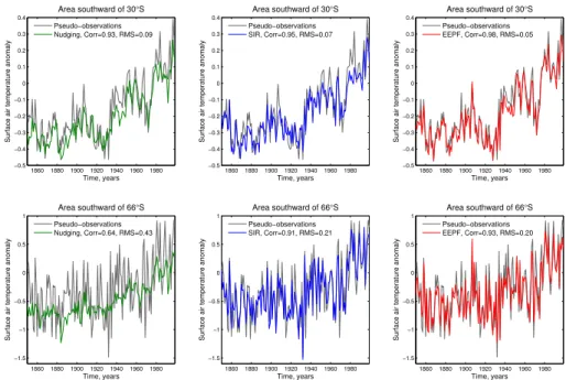
We examine the reconstructions of surface air temperature averaged over two do-20

mains: the area southward of 30◦S and the area southward of 66◦S (the top and bottom panels of Fig. 1). Reasonable reconstructions of surface air temperature are obtained using either the sequential importance resampling filter (blue curve) or the extremely efficient particle filter (red curve) over both domains. For the area southward of 30◦S shown in the top panel of Fig. 1, the correlations for the sequential importance resam-25

(12)

CPD

9, 43–74, 2013

Title Page

Tables Figures

◭ ◮

Back Close

Full Screen / Esc

Discussion

P

a

per

|

Dis

cussion

P

a

per

|

Discussion

P

a

per

|

Discussio

n

P

a

per

|

nudging performs also very well for the area southward of 30◦S (green curve in the top panel of Fig. 1) providing with correlation of 0.93 and the RMS error of 0.09◦C. But for the area southward of 66◦S shown in the bottom panel of Fig. 1, its performance is weaker: correlation is 0.64 and the RMS error is 0.43◦C. Moreover, the variance of the reconstructed anomaly (green curve) is smaller than the variance of the pseudo-5

observations (grey curve). This is due to the fact that the ocean covers a small fraction of the surface southward of 66◦S; therefore, since the nudging is done over the ocean only, it has a weaker direct influence on this area and propagation of the signal from the ocean to the land is not strong enough to lead to high correlations.

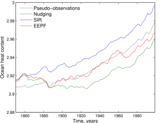
For estimating the performance of a data-assimilation method for the ocean recon-10

struction we consider ocean heat content. Figure 2 illustrates that ocean heat content is not significantly altered by the sequential importance resampling filter. Therefore, the sequential importance resampling filter does not change the heat budget of the climate model. Since the same forcing is used for deriving the pseudo-observations and when performing the data-assimilation experiments, ocean heat content from the 15

sequential importance resampling filter is parallel to the pseudo-observations reflect-ing the influence of different initial conditions during the whole period. The nudging, on the contrary, has a strong influence on ocean heat content. This is due to the way the nudging is implemented: it adjusts heat fluxes from the atmosphere to the ocean. Con-sequently, ocean temperature changes, so does ocean heat content. The extremely 20

efficient particle filter obtains ocean heat content that lies between the one from the nudging and the one from the sequential importance resampling filter and appears to be the closest to the pseudo-observations. To address the robustness of this result, we perform four experiments using different initial conditions for each data-assimilation method and investigate the RMS errors between ocean heat content reconstructed 25

(13)

CPD

9, 43–74, 2013

Title Page

Tables Figures

◭ ◮

Back Close

Full Screen / Esc

Discussion

P

a

per

|

Dis

cussion

P

a

per

|

Discussion

P

a

per

|

Discussio

n

P

a

per

|

ocean heat content from the extremely efficient particle filter has the smallest mean RMS error.

Next, we investigate the skill of the assimilation methods in reconstructing spatial features. In order to do that, we compute first empirical orthogonal functions (EOFs) of the pseudo-observations and project the results of model simulations onto them. Then, 5

the corresponding principal components (PCs) and the projections are compared by means of correlation. We perform four experiments using different initial conditions for every data-assimilation method. The EOFs are computed for winter period (from May until October) over the area southward of 60◦S, as we are mainly interested in the regions that are ice covered or that are close to the ice edge, and over a 21-yr period, 10

since it is long enough to capture the main features of the state by the EOFs and short enough to split one model run in several such periods. Therefore, we divide a 150-yr run in six 21-yr periods starting from year 1865 and ending in year 1990, skipping the first 15 yr to avoid the bias induced by the initial conditions. Performing the EOF analysis over six 21-yr periods from four different experiments gives twenty-four correlations for 15

every data-assimilation method.

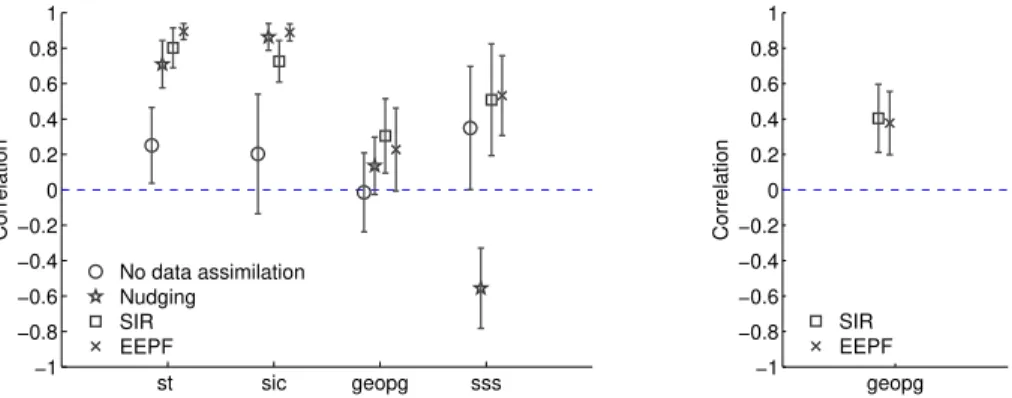
In Fig. 3, we plot mean correlations plus and minus one standard deviation for diff er-ent variables and different data-assimilation methods. When reconstructing surface air temperature (st) or sea ice concentration (sic) all three methods perform rather well pro-viding with high correlations, as shown in the left panel of Fig. 3. Even a free model run 20

(without data assimilation) has positive correlations, which is due to the employment of the same forcing when deriving the pseudo-observations. The skill of the extremely efficient particle filter when reconstructing surface air temperature is only slightly higher than the skill of the sequential importance resampling filter, as it is seen in the left panel of Fig. 3. When reconstructing sea ice concentration, however, the extremely efficient 25

(14)

CPD

9, 43–74, 2013

Title Page

Tables Figures

◭ ◮

Back Close

Full Screen / Esc

Discussion

P

a

per

|

Dis

cussion

P

a

per

|

Discussion

P

a

per

|

Discussio

n

P

a

per

|

efficient particle filter have the higher skills than the sequential importance resampling filter.

Changes in atmospheric circulation is an important characteristics of past climate variability (e.g. Lefebvre and Goosse, 2008; Yuan and Li, 2008). Pressure observations that can be used to constrain the model in order to get reliable estimations of atmo-5

spheric circulation are, however, very limited for paleoclimate applications. Therefore, we investigate the skill of the atmospheric circulation reconstructions when surface air temperature is assimilated. We perform the EOF analysis for geopotential height, the variable in LOVECLIM that represents atmospheric circulation. In the left panel of Fig. 3, we see that correlations for geopotential height (geopg) are overall positive but 10

not significant. To address this issue, we perform experiments with assimilating the pseudo-observations over a smaller domain: the area southward of 60◦S instead of the area southward of 30◦S. In the right panel of Fig. 3, we see that correlations for geopotential height are higher when the assimilation domain is smaller. This is due to a smaller number of degrees of freedom when assimilating over a smaller domain, 15

which means that the particle filters are still close to degeneracy.

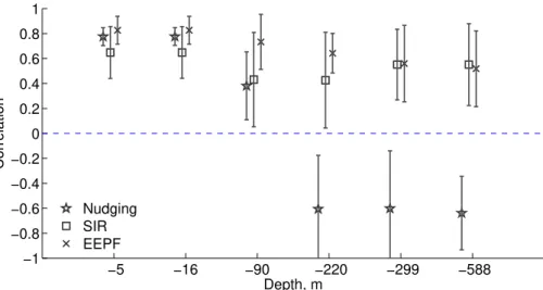
To continue with assessment of the performance of a data-assimilation method when reconstructing the ocean state, we perform the EOF analysis of sea surface salinity (sss), whose variations play a crucial role in the changes in density and, consequently, in the oceanic circulation and the vertical stability of the water column (e.g. Martinson, 20

1990; Gordon, 1991). In the left panel of Fig. 3, we see that the extremely efficient parti-cle filter and the sequential importance resampling filter provide with positive and rather good correlations, taken into account that sea surface salinity is not directly linked to assimilated surface air temperature. By contrast, sea surface salinity obtained by the nudging has always negative correlations with the pseudo-observations. In order to 25

(15)

CPD

9, 43–74, 2013

Title Page

Tables Figures

◭ ◮

Back Close

Full Screen / Esc

Discussion

P

a

per

|

Dis

cussion

P

a

per

|

Discussion

P

a

per

|

Discussio

n

P

a

per

|

the nudging term strongly modifies the mixing (not shown) leading to a wrong vertical ocean temperature profile and to wrong vertical salinity.

5 Assimilation of the sparse pseudo-observations

In the following experiments, we investigate the performance of the data-assimilation methods when the pseudo-observations are as sparse as the dataset HADCRUT3 5

of the instrumental surface temperature records over the last 150 yr (Brohan et al., 2006) by selecting the pseudo-observations at the same locations as the HADCRUT3 dataset. The resolution of these pseudo-observations changes in time: for example, for year 1850 around 10 pseudo-observations are located in the area southward of 60◦S and for year 2000 it is about 80. The number of the sparse pseudo-observations in 10

the area southward of 60◦S is substantially smaller compared to the area southward of 30◦S: 80 sparse pseudo-observations against 400 for year 2000, for example. Since we are interested in the climate state reconstruction over the area southward of 60◦S and the number of the sparse pseudo-observations in this area is very small, the prior distribution has to be chosen such that it increases the relative importance of the sparse 15

pseudo-observations located in the area 90◦S–60◦S compared to the sparse pseudo-observations located in the area 60◦S–30◦S or decrease the data-assimilation area. Here, we keep the prior distribution to be uniform but assimilate the sparse pseudo-observations over a smaller area: the area southward of 60◦S. The nudging, however, is still applied over the global ocean.

20

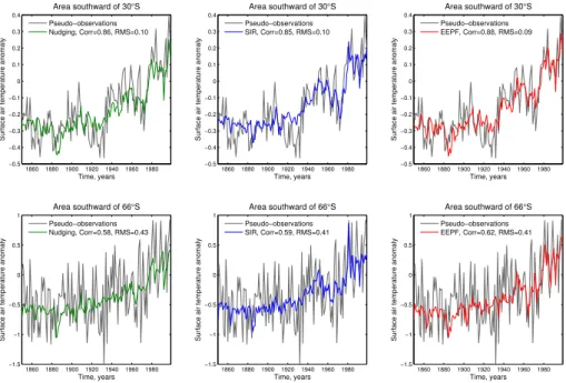
In Fig. 5, we plot time series of surface air temperature anomalies averaged over the area southward of 30◦S (the top panel) and over the area southward of 66◦S (the bottom panel). Compared to the case of assimilating the dense dataset of the pseudo-observations, the variance of the anomalies is underestimated, which is due to the sparse net of the pseudo-observations. Annan and Hargreaves (2012) has also 25

(16)

CPD

9, 43–74, 2013

Title Page

Tables Figures

◭ ◮

Back Close

Full Screen / Esc

Discussion

P

a

per

|

Dis

cussion

P

a

per

|

Discussion

P

a

per

|

Discussio

n

P

a

per

|

surface air temperature averaged over the area southward of 30◦S: correlations are 0.86, 0.85, and 0.88 for the nudging, the sequential importance resampling filter, and the extremely efficient particle filter, respectively, while for the model without any data assimilation correlation is 0.78. In the area southward of 66◦S where only a few pseudo-observations are located, we have a good estimation of the trend but not of the vari-5

ance. Moreover, the trend reconstruction is achieved mainly due to the well-defined forcing not due to data assimilation. Indeed, when no data assimilation is used cor-relation is 0.56 and corcor-relations obtained by the data-assimilation methods are 0.58, 0.59, and 0.62 for the nudging, the sequential importance resampling filter, and the ex-tremely e_fficient particle filter, respectively. It should be mentioned, however, that when 10

the forcing is unknown, the trend can be still estimated due to data assimilation, see Dubinkina et al. (2011).

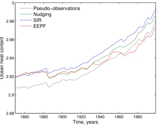
In Fig. 6 we see that ocean heat content obtained by the extremely efficient parti-cle filter appears to be the closest to the pseudo-observations, and ocean heat con-tent obtained by the sequential importance resampling filter is parallel to the pseudo-15

observations. As in the case of assimilating the dense pseudo-observation dataset, we perform five experiments using different initial conditions for each data-assimilation method in order to check the robustness of this result. From these experiments we obtain the following mean RMS errors: 0.007 for the nudging, 0.008 for the extremely efficient particle filter, and 0.009 for the sequential importance resampling filter. Hence, 20

the mean RMS errors are comparable, unlike in the case of assimilating the dense pseudo-observations when the extremely efficient particle filter provides with the mean RMS error much smaller than any other method (0.008 against 0.013 or 0.014).

For examining the spatial skill of the data-assimilation methods, we perform the EOF analysis as described in Sect. 4, but since resolution of the sparse pseudo-25

(17)

CPD

9, 43–74, 2013

Title Page

Tables Figures

◭ ◮

Back Close

Full Screen / Esc

Discussion

P

a

per

|

Dis

cussion

P

a

per

|

Discussion

P

a

per

|

Discussio

n

P

a

per

|

pseudo-observations and projections of model simulations onto the corresponding first EOFs of the pseudo-observations. Mean and standard deviation are computed over five correlations.

Figure 7 illustrates that the extremely efficient particle filter provides overall with higher correlations than any other method when reconstructing surface air tempera-5

ture. Compared to the case of assimilating the dense pseudo-observation dataset, as-similation of the sparse pseudo-observations results in smaller mean correlations and larger standard deviations, except for the period 1970–1990, at which many pseudo-observations are available.

In Fig. 8, we see that even for the end of the 19th century, when the pseudo-10

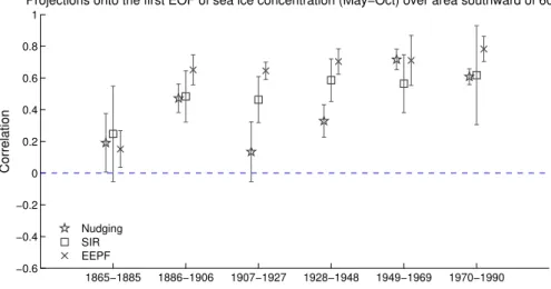
observations are very sparse, correlations given by the extremely e_fficient particle filter and by the sequential importance resampling filter are quite reasonable for sea ice con-centration, unlike the correlations given by the nudging. Moreover, the extremely effi -cient particle filter reconstructs sea ice concentration better than the sequential impor-tance resampling filter, like in the case of assimilating the dense pseudo-observations. 15

From Fig. 9 we see that the data-assimilation methods do not constrain the model well enough in order to have reliable estimations of atmospheric circulation. Only in the period 1970–1990 with many pseudo-observations, correlations improve and become comparable to the correlations for geopotential height when assimilating the dense pseudo-observation dataset over the area southward of 60◦S (the right panel of Fig. 3). 20

When reconstructing sea surface salinity, which is shown in Fig. 10, the extremely ef-ficient particle filter performs quite well together with the sequential importance resam-pling filter. Over some periods the extremely efficient particle filter gives higher correla-tions, over other periods it is the sequential importance resampling filter that provides with higher correlations. The nudging performs worse than any particle filter, and over 25

(18)

CPD

9, 43–74, 2013

Title Page

Tables Figures

◭ ◮

Back Close

Full Screen / Esc

Discussion

P

a

per

|

Dis

cussion

P

a

per

|

Discussion

P

a

per

|

Discussio

n

P

a

per

|

6 Conclusions

We have shown that the extremely efficient particle filter provides with quite encour-aging results: global variables like ocean heat content and surface air temperature averaged over large domains are well estimated. When assimilating the dense pseudo-observation dataset, the extremely efficient particle filter provides with reasonable re-5

constructions of not only variables that are directly linked to the pseudo-observations of surface air temperature, as surface air temperature and sea ice concentration, but also variables as geopotential height and sea surface salinity. Reliable reconstructions of the latter variables are essential for paleoclimate applications since the observations of pressure and salinity are limited there. Moreover, these reconstructions give good 10

perspectives for initializing climate predictions.

When assimilating the sparse pseudo-observations that are given at the same lo-cations as the dataset of instrumental surface temperature records HADCRUT3, the performance of the extremely efficient particle filter is weaker due to the limited num-ber of the pseudo-observations. Nevertheless, even at the end of the 19th century, the 15

reconstructions of surface air temperature and of sea ice concentration are quite good. The reconstructions of geopotential height and of sea surface salinity display, however, a lower skill.

Overall, the extremely e_fficient particle filter achieves better or equivalent results compared to the sequential importance resampling filter. To be more precise, surface 20

air temperature reconstructed by the sequential importance resampling filter has al-ready high correlations with the pseudo-observations, and the extremely e_fficient parti-cle filter introduces only a slight improvement. In reconstructing sea ice concentration, however, a clear improvement is accomplished by the extremely efficient particle filter compared to the sequential importance resampling filter. When it comes to the recon-25

(19)

CPD

9, 43–74, 2013

Title Page

Tables Figures

◭ ◮

Back Close

Full Screen / Esc

Discussion

P

a

per

|

Dis

cussion

P

a

per

|

Discussion

P

a

per

|

Discussio

n

P

a

per

|

the sequential importance resampling filter is equivalent to the performance of the ex-tremely e_fficient particle filter.

Even though the nudging used here provides with good reconstructions of surface air temperature and of sea ice concentration, it has the drawback of not respecting the dynamics of the ocean, which results in the wrong vertical profile of ocean temperature 5

and, consequently, in wrong pattern of sea surface salinity. Nudging of salinity and ocean temperature over the depth could be a possible solution to this problem, but it should be kept in mind that observations of deep ocean temperature and salinity are available only for the recent past.

The improvement brought by the extremely efficient particle filter is apparent, which 10

makes a strong argument for the use of the extremely e_fficient particle filter in the climate state reconstruction. Some developments, however, are still needed in order to get reliable estimations of variables that are not strongly linked through the model dynamics to the assimilated surface air temperature such as geopotential height and salinity.

15

Acknowledgements. H. Goosse is Senior Research Associate with the F.R.S.-FNRS-Belgium. The research leading to these results has received funding from the F.R.S.-FNRS, the Bel-gian Federal Science Policy Office and the European Union’s Seventh Framework programme (FP7/2007–2013) under grant agreement no. 243908, “Past4Future. Climate change – Learn-ing from the past climate”. This is Past4Future contribution no. X.

20

References

Annan, J. D. and Hargreaves, J. C.: Identification of climatic state with limited proxy data, Clim. Past, 8, 1141–1151, doi:10.5194/cp-8-1141-2012, 2012. 44, 46, 57

Bhend, J., Franke, J., Folini, D., Wild, M., and Br ¨onnimann, S.: An ensemble-based approach to climate reconstructions, Clim. Past, 8, 963–976, doi:10.5194/cp-8-963-2012, 2012. 44 25

(20)

CPD

9, 43–74, 2013

Title Page

Tables Figures

◭ ◮

Back Close

Full Screen / Esc

Discussion

P

a

per

|

Dis

cussion

P

a

per

|

Discussion

P

a

per

|

Discussio

n

P

a

per

|

Brovkin, V., Bendtsen, J., Claussen, M., Ganopolski, A., Kubatzki, C., Petoukhov, V., and An-dreev, A.: Carbon cycle, vegetation and climate dynamics in the Holocene: experiments with the CLIMBER-2 model, Global. Biogeochem. Cy., 16, 1139, doi:10.1029/2001GB001662, 2002. 52

Courtier, P., Th ´epaut, J.-N., and Hollingsworth, A.: A strategy for operational implementa-5

tion of 4D-VAR, using an incremental approach, Q. J. Roy. Meteor. Soc., 120, 1367–1387, doi:10.1002/qj.49712051912, 1994. 45

Dubinkina, S., Goosse, H., Sallaz-Damaz, Y., Crespin, E., and Crucifix, M.: Testing a particle filter to reconstruct climate changes over the past centuries, Int. J. Bifurcat. Chaos, 21, 3611– 3618, doi:10.1142/S0218127411030763, 2011. 47, 52, 53, 58

10

Evensen, G.: Sequential data assimilation with a nonlinear quasi-geostrophic model using Monte Carlo methods to forecast error statistics, J. Geophys. Res., 99, 10143–10162, doi:10.1029/94JC00572, 1994. 45

Goosse, H. and Fichefet, T.: Importance of ice-ocean interactions for the global ocean circula-tion: a model study, J. Geophys. Res., 104, 23337–23355, 1999. 52

15

Goosse, H., Lefebvre, W., de Montety, A., Crespin, E., and Orsi, A.: Consistent past half-century trends in the atmosphere, the sea ice and the ocean at high southern latitudes, Clim. Dynam., 33, 999–1016, doi:10.1007/s00382-008-0500-9, 2009. 46

Goosse, H., Brovkin, V., Fichefet, T., Haarsma, R., Huybrechts, P., Jongma, J., Mouchet, A., Selten, F., Barriat, P.-Y., Campin, J.-M., Deleersnijder, E., Driesschaert, E., Goelzer, H., 20

Janssens, I., Loutre, M.-F., Morales Maqueda, M. A., Opsteegh, T., Mathieu, P.-P., Munhoven, G., Pettersson, E. J., Renssen, H., Roche, D. M., Schaeffer, M., Tartinville, B., Timmer-mann, A., and Weber, S. L.: Description of the Earth system model of intermediate complex-ity LOVECLIM version 1.2, Geosci. Model Dev., 3, 603–633, doi:10.5194/gmd-3-603-2010, 2010. 52

25

Goosse, H., Crespin, E., Dubinkina, S., Loutre, M., Mann, M., Renssen, H., Sallaz-Damaz, Y., and Shindell, D.: The role of forcing and internal dynamics in explaining the “Medieval Climate Anomaly”, Clim. Dynam., 39, 2847–2866, doi:10.1007/s00382-012-1297-0, 2012. 48 Gordon, A.: Two Stable Modes of Southern Ocean Winter Stratification, in: Deep Convection

and Deep Water Formation in the Oceans Proceedings of the International Monterey Col-30

(21)

CPD

9, 43–74, 2013

Title Page

Tables Figures

◭ ◮

Back Close

Full Screen / Esc

Discussion

P

a

per

|

Dis

cussion

P

a

per

|

Discussion

P

a

per

|

Discussio

n

P

a

per

|

Hoke, J. and Anthes, R.: The initialization of numerical models by a dynamic relaxation tech-nique, Mon. Weather Rev., 104, 1551–1556, 1976. 49

Keenlyside, N., Latif, M., Jungclaus, J., Kornblueh, L., and Roeckner, E.: Advanc-ing decadal-scale climate prediction in the North Atlantic sector, Nature, 53, 84–88, doi:10.1038/nature06921, 2008. 47

5

Lefebvre, W. and Goosse, H.: An analysis of the atmospheric processes driving the large-scale winter sea-ice variability in the Southern Ocean, J. Geophys. Res., 113, C02004, doi:10.1029/2006JC004032, 2008. 56

Martinson, D.: Evolution of the Southern Ocean winter mixed layer and sea ice: open ocean deepwater formation and ventilation, J. Geophys. Res., 95, 11641–11654, 10

doi:10.1029/JC095iC07p11641, 1990. 56

Opsteegh, J., Haarsma, R., Selten, F., and Kattenberg, A.: ECBILT: A dynamic alternative to mixed boundary conditions in ocean models, Tellus, 50A, 348–367, doi:10.1034/j.1600-0870.1998.t01-1-00007.x, 1998. 52

Pohlmann, H., Jungclaus, J., K ¨ohl, A., Stammer, D., and Marotzke, J.: Initializing decadal cli-15

mate predictions with the gecco oceanic synthesis: effects on the north atlantic, J. Climate, 22, 3926–3938, doi:10.1175/2009JCLI2535.1, 2009. 47

Smerdon, J.: Climate models as a test bed for climate reconstruction methods: pseudoproxy experiments, WIREs Clim. Change, 3, 63–77, doi:10.1002/wcc.149, 2012. 47

Snyder, C., Bengtsson, T., Bickel, P., and Anderson, J.: Obstacles to high-dimensional particle 20

filtering, Mon. Weather Rev., 136, 4629–4640, doi:10.1175/2008MWR2529.1, 2008. 45 Swingedouw, D., Mignot, J., Labtoulle, S., Guilyardi, E., and Madec, G.: Initialisation and

predictability of the AMOC over the last 50 years in a climate model, Clim. Dynam., doi:10.1007/s00382-012-1516-8, in press, 2013. 47, 50

Talagrand, O.: Assimilation of observations, an introduction, J. Metorol. Soc. JPN, Special Issue 25

75, 191–209, 1997. 45

van Leeuwen, P.: Particle Filtering in Geophysical Systems, Mon. Weather Rev., 137, 4089– 4114, doi:10.1175/2009MWR2835.1, 2009. 49

van Leeuwen, P.: Nonlinear data assimilation in geosciences: an extremely efficientp article filter, Q. J. Roy. Meteor. Soc., 136, 1991–1999, doi:10.1002/qj.699, 2010. 46, 47, 51 30

(22)

CPD

9, 43–74, 2013

Title Page

Tables Figures

◭ ◮

Back Close

Full Screen / Esc

Discussion

P

a

per

|

Dis

cussion

P

a

per

|

Discussion

P

a

per

|

Discussio

n

P

a

per

|

Widmann, M., Goosse, H., van der Schrier, G., Schnur, R., and Barkmeijer, J.: Using data assimilation to study extratropical Northern Hemisphere climate over the last millennium, Clim. Past, 6, 627–644, doi:10.5194/cp-6-627-2010, 2010. 44

Yuan, X. and Li, C.: Climate modes in southern high latitudes and theur impact on Antarctic sea ice, J. Geophys. Res., 113, C06S91, doi:10.1029/2006JC004067, 2008. 56

(23)

CPD

9, 43–74, 2013

S. Dubinkina and H. Goosse Title Page Abstract Introduction Conclusions References Tables Figures ◭ ◮ ◭ ◮ Back Close

Full Screen / Esc

Printer-friendly Version Interactive Discussion Discussion P a per | Dis cussion P a per | Discussion P a per | Discussio n P a per |

1860 1880 1900 1920 1940 1960 1980 −0.5 −0.4 −0.3 −0.2 −0.1 0 0.1 0.2 0.3 0.4 Time, years

Surface air temperature anomaly

Area southward of 30°S Pseudo−observations Nudging, Corr=0.93, RMS=0.09

1860 1880 1900 1920 1940 1960 1980 −0.5 −0.4 −0.3 −0.2 −0.1 0 0.1 0.2 0.3 0.4 Time, years

Area southward of 30°S Pseudo−observations SIR, Corr=0.95, RMS=0.07

1860 1880 1900 1920 1940 1960 1980 −0.5 −0.4 −0.3 −0.2 −0.1 0 0.1 0.2 0.3 0.4 Time, years

Area southward of 30°S Pseudo−observations EEPF, Corr=0.98, RMS=0.05

1860 1880 1900 1920 1940 1960 1980 −1.5 −1 −0.5 0 0.5 1 Time, years

Fig. 1.Grey line: pseudo-observation of surface air temperature anomalies; green line:

(24)

CPD

9, 43–74, 2013

Title Page

Tables Figures

◭ ◮

Back Close

Full Screen / Esc

Discussion

P

a

per

|

Dis

cussion

P

a

per

|

Discussion

P

a

per

|

Discussio

n

P

a

per

|

1860 1880 1900 1920 1940 1960 1980 2.88

2.9 2.92 2.94 2.96 2.98 3

Time, years

Ocean heat content

Pseudo−observations Nudging

SIR EEPF

Fig. 2.Grey line: pseudo-observation of ocean heat content; green line: ocean heat content

(25)

CPD

9, 43–74, 2013

Title Page

Tables Figures

◭ ◮

Back Close

Full Screen / Esc

Discussion

P

a

per

|

Dis

cussion

P

a

per

|

Discussion

P

a

per

|

Discussio

n

P

a

per

|

st sic geopg sss

−1 −0.8 −0.6 −0.4 −0.2 0 0.2 0.4 0.6 0.8 1

Correlation

No data assimilation Nudging

SIR EEPF

geopg −1

−0.8 −0.6 −0.4 −0.2 0 0.2 0.4 0.6 0.8 1

Correlation

SIR EEPF

Fig. 3.Correlations between first PCs of the pseudo-observations and projections of the model

(26)

CPD

9, 43–74, 2013

Title Page

Tables Figures

◭ ◮

Back Close

Full Screen / Esc

Discussion

P

a

per

|

Dis

cussion

P

a

per

|

Discussion

P

a

per

|

Discussio

n

P

a

per

|

−5 −16 −90 −220 −299 −588 −1

−0.8 −0.6 −0.4 −0.2 0 0.2 0.4 0.6 0.8 1

Correlation

Depth, m Nudging

SIR EEPF

Fig. 4.Correlations between first PCs of the pseudo-observations and projections of the model

(27)

CPD

9, 43–74, 2013

S. Dubinkina and H. Goosse Title Page Abstract Introduction Conclusions References Tables Figures ◭ ◮ ◭ ◮ Back Close

Full Screen / Esc

Printer-friendly Version Interactive Discussion Discussion P a per | Dis cussion P a per | Discussion P a per | Discussio n P a per |

1860 1880 1900 1920 1940 1960 1980 −0.5 −0.4 −0.3 −0.2 −0.1 0 0.1 0.2 0.3 0.4 Time, years

1860 1880 1900 1920 1940 1960 1980 −1.5 −1 −0.5 0 0.5 1 Time, years

(28)

CPD

9, 43–74, 2013

Title Page

Tables Figures

◭ ◮

Back Close

Full Screen / Esc

Discussion

P

a

per

|

Dis

cussion

P

a

per

|

Discussion

P

a

per

|

Discussio

n

P

a

per

|

1860 1880 1900 1920 1940 1960 1980 2.88

2.9 2.92 2.94 2.96 2.98 3

Time, years

Ocean heat content

Pseudo−observations Nudging

SIR EEPF

(29)

CPD

9, 43–74, 2013

Title Page

Tables Figures

◭ ◮

Back Close

Full Screen / Esc

Discussion

P

a

per

|

Dis

cussion

P

a

per

|

Discussion

P

a

per

|

Discussio

n

P

a

per

|

1865−1885 1886−1906 1907−1927 1928−1948 1949−1969 1970−1990

−0.6 −0.4 −0.2 0 0.2 0.4 0.6 0.8 1

Correlation

Projections onto the first EOF of surface air temperature (May−Oct) over area southward of 60°S

Nudging SIR EEPF

Fig. 7.Correlations between first PCs of the pseudo-observations and projections of model

(30)

CPD

9, 43–74, 2013

Title Page

Tables Figures

◭ ◮

Back Close

Full Screen / Esc

Discussion

P

a

per

|

Dis

cussion

P

a

per

|

Discussion

P

a

per

|

Discussio

n

P

a

per

|

1865−1885 1886−1906 1907−1927 1928−1948 1949−1969 1970−1990

−0.6 −0.4 −0.2 0 0.2 0.4 0.6 0.8 1

Correlation

Projections onto the first EOF of sea ice concentration (May−Oct) over area southward of 60°S

Nudging SIR EEPF

(31)

CPD

9, 43–74, 2013

Title Page

Tables Figures

◭ ◮

Back Close

Full Screen / Esc

Discussion

P

a

per

|

Dis

cussion

P

a

per

|

Discussion

P

a

per

|

Discussio

n

P

a

per

|

1865−1885 1886−1906 1907−1927 1928−1948 1949−1969 1970−1990

−0.6 −0.4 −0.2 0 0.2 0.4 0.6 0.8 1

Correlation

Projections onto the first EOF of atmospheric circulation (May−Oct) over area southward of 60°S

Nudging SIR EEPF

(32)

CPD

9, 43–74, 2013

Title Page

Tables Figures

◭ ◮

Back Close

Full Screen / Esc

Discussion

P

a

per

|

Dis

cussion

P

a

per

|

Discussion

P

a

per

|

Discussio

n

P

a

per

|

1865−1885 1886−1906 1907−1927 1928−1948 1949−1969 1970−1990

−0.6 −0.4 −0.2 0 0.2 0.4 0.6 0.8 1

Correlation

Projections onto the first EOF of sea surface salinity (May−Oct) over area southward of 60°S

Nudging SIR EEPF