❊♥s❛✐♦s ❊❝♦♥ô♠✐❝♦s
❊s❝♦❧❛ ❞❡
Pós✲●r❛❞✉❛çã♦
❡♠ ❊❝♦♥♦♠✐❛
❞❛ ❋✉♥❞❛çã♦
●❡t✉❧✐♦ ❱❛r❣❛s
◆◦ ✸✾✶ ■❙❙◆ ✵✶✵✹✲✽✾✶✵
▼❛❝r♦ ❙❤♦❝❦s ❛♥❞ ▼✐❝r♦❡❝♦♥♦♠✐❝ ■♥st❛❜✐❧✲
✐t②✿ ❛♥ ❊♣✐s♦❞✐❝ ❆♥❛❧②s✐s ♦❢ ❇♦♦♠s ❛♥❞ ❘❡✲
❝❡ss✐♦♥s
▼❛r❝❡❧♦ ❈♦rt❡s ◆❡r✐✱ ▼❛r❦ ❘✳ ❚❤♦♠❛s
♦♣✐♥✐õ❡s ♥❡❧❡s ❡♠✐t✐❞❛s ♥ã♦ ❡①♣r✐♠❡♠✱ ♥❡❝❡ss❛r✐❛♠❡♥t❡✱ ♦ ♣♦♥t♦ ❞❡ ✈✐st❛ ❞❛
❋✉♥❞❛çã♦ ●❡t✉❧✐♦ ❱❛r❣❛s✳
❊❙❈❖▲❆ ❉❊ PÓ❙✲●❘❆❉❯❆➬➹❖ ❊▼ ❊❈❖◆❖▼■❆ ❉✐r❡t♦r ●❡r❛❧✿ ❘❡♥❛t♦ ❋r❛❣❡❧❧✐ ❈❛r❞♦s♦
❉✐r❡t♦r ❞❡ ❊♥s✐♥♦✿ ▲✉✐s ❍❡♥r✐q✉❡ ❇❡rt♦❧✐♥♦ ❇r❛✐❞♦ ❉✐r❡t♦r ❞❡ P❡sq✉✐s❛✿ ❏♦ã♦ ❱✐❝t♦r ■ss❧❡r
❉✐r❡t♦r ❞❡ P✉❜❧✐❝❛çõ❡s ❈✐❡♥tí✜❝❛s✿ ❘✐❝❛r❞♦ ❞❡ ❖❧✐✈❡✐r❛ ❈❛✈❛❧❝❛♥t✐
❈♦rt❡s ◆❡r✐✱ ▼❛r❝❡❧♦
▼❛❝r♦ ❙❤♦❝❦s ❛♥❞ ▼✐❝r♦❡❝♦♥♦♠✐❝ ■♥st❛❜✐❧✐t②✿ ❛♥
❊♣✐s♦❞✐❝ ❆♥❛❧②s✐s ♦❢ ❇♦♦♠s ❛♥❞ ❘❡❝❡ss✐♦♥s✴ ▼❛r❝❡❧♦ ❈♦rt❡s ◆❡r✐✱ ▼❛r❦ ❘✳ ❚❤♦♠❛s ✕ ❘✐♦ ❞❡ ❏❛♥❡✐r♦ ✿ ❋●❱✱❊P●❊✱ ✷✵✶✵
✭❊♥s❛✐♦s ❊❝♦♥ô♠✐❝♦s❀ ✸✾✶✮
■♥❝❧✉✐ ❜✐❜❧✐♦❣r❛❢✐❛✳
$Q(SLVRGLF$QDO\VLVRI%RRPVDQG5HFHVVLRQV
Marcelo C. Neri 1
and
Mark R. Thomas 2
-XO\
±,QWURGXFWLRQ
Income redistribution is difficult. In part this stems from the natural political resistance that forms in response to any attempt to take resources away from one group in a society, as redistribution entails. However, politically the easier part, the reallocation of those resources to their intended recipients, often presents a technical challenge at least as great as the political challenge of raising them. Transfer schemes have to be correctly targeted. Labor-market interventions generate incentive effects that may diminish their effects. Service provision depends on building the necessary institutional means.
If income redistribution presents a challenge, it is appealing to think that economic growth presents a politically, and perhaps even technically, simpler way of reducing poverty. One question, to which this paper aims to provide clues, is to what extent this is realistic in Brazil. Between 1982 and the present, the period we shall cover in this paper, there have been several periods of significant growth in Brazil. In the three year period 1993-95, for example, per-capita income grew at an average of 3.5 percent annually. These periods of growth have reduced the numbers in poverty. By some estimates, the poverty headcount decreased by
about 20 percent in the year following the introduction of the real.3
There have also been some severe recessions. These have undone some of the gains in the fight against poverty that were made during the good times. In the three year period from
1 Marcelo Neri ([email protected]
) is Professor at EPGE / FGV and Head of the Center of Social Policies (CPS) at IBRE / FGV in Rio de Janeiro.
2
Mark R. Thomas is Economist at World Bank, in Brasília.
1990-92, per-capita income declined by about 2.7 percent annually. By one measure, the poverty headcount rose by nearly half.
By contrasting episodes of contraction with growth, one can gain insights about the effects of economic events on Brazilian households. A related matter is the effect of volatility on individuals’ welfare. One dimension of volatility is its (no doubt deleterious) effect on economic growth: we shall not address that important macroeconomic issue here. But for a given growth rate, volatility also has effects on income distribution and on the variability of individuals’ earnings, which we shall evaluate.
The vehicle for such an analysis is the monthly employment survey (Pesquisa de Emprego Mensal, henceforth PME). This survey visits the same households eight times in a 16-month period (four monthly visits, an eight month hiatus, then four more visits). Such a design reveals changes in individuals’ circumstances—income, employment—and we shall use this feature to analyze the effects of episodes of growth and recession. Since the PME is
conducted only in six Brazil’s largest metropolitan areas,4 our conclusions will only be valid
for metropolitan Brazil; not rural or even urban Brazil outside the large cities.
We shall consider seven periods, three of growth—two booms and one period of recovery after stabilization—and four of recession, and from this sample try to make general statements about the effects of booms and recessions on income distribution, employment, and poverty.
The three periods of growth are:
• January 1984 to June 1985: recovery after the debt crisis
• January 1986 to March 1987: the cruzado boom
• January 1994 to May 1995: the real boom.
The four periods of recession or stagnation are:
• June 1982 to December 1983: the first debt crisis
• January 1990 to March 1991: the Collor plan
• July 1996 to December 1997: the Asian crisis
• January 1998 to June 1999: the real devaluation.
There is a great deal that is different about each of these periods when compared with the others. Indeed, in order to reflect on this, the next section gives a brief outline of the events surrounding each: very brief since there has been plenty written elsewhere chronicling these episodes. However, we shall also be looking for common features across the episodes in both categories: it turns out that such common features do exist in the PME data.
Finally the paper will make two excursions into specificity. First, we examine the impact, during a period of stable and strong growth, of an increase in the minimum wage, which was raised from 70 reais to 100 reais in May 1995. Second, we discuss the effects of the recent recession, and surmise a little on the implications of the PME data for social protection policy in Brazil.
The second section, following this one, gives an outline of each period studied. The third section presents the simple effects of growth and recession on wage income and its distribution. The fourth section presents a more complex analysis of employment flows, the role of the informal sector, and transitions in and out of poverty. The fifth section briefly discusses the empirical effects of the 1995 minimum wage increase. The sixth and final section concludes with some general lessons and some specific comments about the current economic environment in Brazil.
±6HYHQ(SLVRGHVRIWKH%UD]LOLDQ(FRQRP\
&KDUWSelected Macroeconomic Time Series
A - Unemployment Rates B - Inflation Rates
0.02 0.03 0.04 0.05 0.06 0.07 0.08 0.09 0.10 Jun/ 80 M ai/8 1 Ab r/ 8 2 Ma r/ 83 F ev/ 84 Ja n/ 85 Dez/8 5 N ov/ 86 O u t/8 7 Set/8 8 A go/ 89 Ju l/9 0 Jun/ 91 M ai/9 2 Ab r/ 9 3 Ma r/ 94 F ev/ 95 Ja n/ 96 Dez/9 6 N ov/ 97 O u t/9 8 -0.10 0.00 0.10 0.20 0.30 0.40 0.50 0.60 0.70 0.80 0.90 Jun/ 80 M ai/8 1 Ab r/ 8 2 Ma r/ 83 F ev/ 84 Ja n/ 85 Dez/8 5 N ov/ 86 O u t/8 7 Set/8 8 A go/ 89 Ju l/9 0 Jun/ 91 M ai/9 2 Ab r/ 9 3 Ma r/ 94 F ev/ 95 Ja n/ 96 Dez/9 6 N ov/ 97 O u t/9 8 6RXUFH30(,%*( 6RXUFH,13&,%*(
C - Gini Coefficient D - GDP
(Universe : Active Age Population - Total Labor
0.55 0.56 0.57 0.58 0.59 0.60 0.61 0.62 0.63 0.64 Ju n/ 80 M ai/ 81 Ab r/8 2 M ar/ 83 Fe v/8 4 Ja n/ 85 De z/8 5 No v/8 6 Ou t/8 7 Se t/8 8 Ag o/ 89 Jul /9 0 Ju n/ 91 M ai/ 92 Ab r/9 3 M ar/ 94 Fe v/9 5 Ja n/ 96 De z/9 6 No v/9 7 Ou t/9 8 80.00 90.00 100.00 110.00 120.00 130.00 140.00 150.00 160.00 Ju n/ 80 M ai/ 81 Ab r/8 2 M ar/ 83 Fe v/8 4 Ja n/ 85 De z/8 5 No v/8 6 Ou t/8 7 Se t/8 8 Ag o/ 89 Jul /9 0 Ju n/ 91 M ai/ 92 Ab r/9 3 M ar/ 94 Fe v/9 5 Ja n/ 96 De z/9 6 No v/9 7 Ou t/9 8 6RXUFH30(,%*( 6RXUFH&HQWUDO%DQN
The following is included to provide context for the analysis in the rest of the paper. No attempt is made at a complete account of macroeconomic events over the past two decades.
The Latin American Debt Crisis
Stabilization Post Devaluation
In 1983 Brazil signed an agreement with the IMF to cut public spending and devalue the currency. Initially output decreased, and the devaluation fed into inflation through the price of imports. By the period used for this study, however, the economy was in a modest export-led recovery, with unemployment and poverty initially at high points but falling. In 1985, fiscal and monetary policies were relaxed and price controls were introduced. These did not last, however, and inflation rose through the second half of 1985.
The Cruzado Plan Boom
Despite output growth in 1984-85, monthly inflation remained above 10 percent until the introduction of the cruzado in March 1986. The stabilization was attempted with a combination of a fixed exchange rate and price controls. Expansionary fiscal and monetary policy heralded a period of swift but unsustainable consumption-led growth. As with the real stabilization in 1994, the combination of price stabilization and a minimum wage increase (in March 1987) reduced poverty and fed consumption. Trade deficits eventually forced the abandonment of the fixed exchange rate and the late 1980s were marked by a series of failed stabilization plans and repeated bouts of hyperinflation.
The Collor Plan
In the wake of the failure of the cruzado plan, the successive stabilization attempts of the late 1980s had foundered on lack of fiscal control. Introduced in March 1990, the Collor plan combined a new attempt at stabilization with structural reforms. Prices were again frozen and the exchange rate fixed, an attempt was made to abolish formal-sector wage indices, and trade was liberalized, with the average external tariff falling from over 50 percent to 14 percent. In an attempt to rein in inflation, two-thirds of the money supply (as defined by M4) was legally defined as illiquid assets. This monetary contraction produced a severe recession, and poverty increased markedly. After the severe recession of 1990-92, a period of relaxed fiscal and monetary policy followed through 1993, during which time inflation steadily rose and poverty indicators deteriorated even further.
The Real Plan Boom
The Asian Crisis
The loss of confidence caused by the Asian financial crisis placed renewed pressure on the real. Higher interest rates and continued willingness on the part of foreign investors to finance the deficit allowed continued but weak growth. Weakening commodity prices added to the trade deficit and depressed demand.
The Real Devaluation
Investor reaction to the Russian default finally forced the abandonment of the crawling peg in January 1999. The Central Bank raised interest rates to check inflationary pressure owing to rising import prices. In the event, inflation remained in check, interest rates were allowed to fall faster than initially expected, and the subsequent recession has been less acute than feared. Exports have responded sluggishly to the devaluation, however, and commodity prices remain depressed. The real has weakened through the second half of 1999 as the trade deficit has persisted and international investors remained concerned about fiscal sustainability. The period studied in this paper, to January 1998 to June 1999, captures probably the worst of the recession.
,QFRPH*DLQVDQG/RVVHV
The PME data allow us to calculate measures of wage income, and thus changes in income, for individuals and households in the sample. Wage income is of course not total income, let alone consumption or welfare. It nevertheless gives us an indication of the impact of a period of economic growth (or a recession) on an individual or household. In what
follows we work with household per-capita income, averaged over a four-month period,5 and
restrict our sample to household heads.6 We then calculate earnings changes for each
household head between the second four-month period (months 13-16) and the first (months 1-4). Averaging over four month periods before calculating the difference has two advantages. First, this minimizes the effects of measurement error on estimates of the wage. Second, a four-month average wage is probably a more accurate measure of the worker’s welfare than a single monthly-wage observation. Monthly wages fluctuate considerable, and both economic theory and empirical observation suggest that consumption, which is more closely related to welfare than income, fluctuates much less month to month.
We split the sample into earnings quintiles for much of the analysis in order to assess the distributive effects of episodes. It is incorrect to use reported earnings in the same period as the analysis of income changes in order to perform this split. To see why, consider a worker who receives a negative wage shock (falls ill, for example) in the first period. This worker is thus more likely to fall into a low income bracket. He is also more likely to post a wage gain in the following period (he will probably not be ill again). Summing over workers, such effects would generate spurious income gains among the lower income brackets, regardless of the episode in question. Measurement error in wages would generate the same
5 We performed the analysis in four ways and only present one here. The period over which income is
measured—a four-month average or a single month’s observation—and the definition of income—household per-capita or individual income—are both parameters which can vary. Other possibilities of course exist, notably extending the analysis beyond household heads. As far as we have established, none of the conclusions presented are very sensitive to these issues.
6
effect. The solution we adopt is to define quintiles according to a predicted estimate of
income: a function of attributes of the worker and the worker’s sector of employment.7
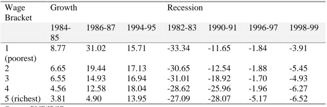
Table 1 shows income gains and losses by quintile for the seven periods. Among the recessions it stands out that recorded income losses since 1996, both at the onset of the Asian crisis and later after the Russian default, do not compare in severity with the recessions of 1982-83 and 1990-91. This is not to belittle the effect of the current downturn on many poor Brazilians. On average, however, the differences are stark. Among the periods of growth, that associated with the cruzado plan stands out as both the most spectacular and the most pro-poor.
7DEOH
Income Gains and Losses by Wage Bracket (percent)
Wage Bracket
Growth Recession
1984-85
1986-87 1994-95 1982-83 1990-91 1996-97 1998-99
1
(poorest)
8.77 31.02 15.71 -33.34 -11.65 -1.84 -3.91
2 6.65 19.44 17.13 -30.65 -12.54 -1.88 -5.45
3 6.55 14.93 16.94 -31.01 -18.92 -1.70 -4.93
4 4.56 12.58 18.04 -28.62 -25.96 -1.96 -6.27
5 (richest) 3.81 4.90 13.95 -27.09 -28.07 -5.17 -6.52
6RXUFH30(,%*(
Chart 2 illustrates the incidence of the booms, in terms of percentage changes in people’s incomes, graphically. It shows a good deal of diversity in the form of different periods of growth. In all three periods, the poor felt at least as much impact from periods of growth as the rich. Chart 3 shows the recessions, and there is even greater variety. The 1990-91 recession “hit the rich harder” (in percentage terms) while the 1982-83 recession hit the poor hardest. The lines for 1996-97 and 1998-99 show the path of income deteriorating after the jitters from the Russian default, with, perhaps surprisingly, the rich losing a slightly greater fraction of wage income than the poor.
7
Income Gains and Losses
&KDUW Growth &KDUW Recession
0% 5% 10% 15% 20% 25% 30% 35%
1 2 3 4 5
wage bracket 86-87
94-95
84-85
-40% -35% -30% -25% -20% -15% -10% -5% 0%
1 2 3 4 5
wage bracket 82-83
90-91 98-99
96-97
6RXUFH30(,%*(
Chart 2 should not be read as saying that growth reduces inequality. In fact the opposite is generally true. Although growth benefits the poor more in percentage terms, the lion’s share still accrues to the rich. The 1990-91 recession, the worst in the period we are discussing, actually reduced inequality, despite increasing poverty dramatically.
To see this, charts 4-6 describe the incidence of income changes in periods of growth. The pattern of growth was more pro-poor in 1986-87 than in the other two expansions, but the charts clearly illustrate that, in the absence of significant redistribution, Brazilian growth has increased inequality. Typically, about half of income gains during periods of rapid expansion (and not taking into account the effect on government spending on pro-poor programs), accrues to the richest fifth of the population.
Incidence of Growth
&KDUW 84-85 &KDUW 86-87 &KDUW 94-95
0% 10% 20% 30% 40% 50% 60%
1 2 3 4 5
wage bracket
0% 10% 20% 30% 40% 50% 60%
1 2 3 4 5
wage bracket
0% 10% 20% 30% 40% 50% 60%
1 2 3 4 5
wage bracket
If growth has created inequality, is it true to say that, despite their undoubted adverse
impact on the poor, recessions reduce inequality?8 Charts 7-9 present the incidence of income
losses across wage brackets and show that recessions have an even more skewed incidence, in absolute monetary terms, than booms. During periods of marked contraction, about 60 percent of income losses accrued to the richest fifth of the population. The pattern is remarkably constant across the three recessions shown.
Incidence of Recession
&KDUW 82-83 &KDUW 90-91 &KDUW 98-99
-70% -60% -50% -40% -30% -20% -10% 0%
1 2 3 4 5
wage bracket
-70% -60% -50% -40% -30% -20% -10% 0%
1 2 3 4 5
wage bracket
-70% -60% -50% -40% -30% -20% -10% 0%
1 2 3 4 5
wage bracket
6RXUFH30(,%*(
Caveats apply to the interpretation of these graphs. First, the income gains and losses recorded among different groups do not take into account these groups ability to take precautions, such as saving, against such volatility. This ability is almost certainly greater among richer people, but data on wage income will not allow us to analyze this question. Second, it is obvious, but worth stating nonetheless to avoid any possible misunderstandings, that the poor are less able to sustain negative income shocks without forgoing basic needs and experiencing severe declines in welfare.
This said, there are conclusions to be drawn from the analysis so far. The first is that although the rich gain the most income from economic growth, they also lose most income during periods of recession. The second is that the patterns of economic growth and recession have varied significantly over the past two decades. The 1986-87 cruzado boom was the most pro-poor over the period. To jump ahead of ourselves a little, the 1994-95 real boom became significantly pro-poor in this sense only in its later period, and after the increase of the minimum wage. Looking at recessions, the 1982-83 recession hit the poor the hardest, although, since the rich suffered about equal income shocks proportional to their income, the incidence of the income losses occurred mainly among the rich. The 1998-99 recession has actually been mild by these standards, and the PME at least does not provide evidence yet of the 1998 recession being any harder on the poor than previous recessions, which is not to deny that it has caused considerable hardship.
There are differences in how growth and recessions affect workers’ incomes according to whether they are working in formal- or informal-sector jobs (charts 10-11). The obvious expectation, that informal workers suffer greater variability in income, is only true of
8 Of course the answer to this question, for a given pattern of growth, depends on the measure of “inequality”
employed (conta própria) workers, not of informal (sem carteira) employees. Self-employed workers’ incomes have been particularly vulnerable to recessions, whereas informal employees’ incomes show no more, and perhaps less, sensitivity during recessions than formal-sector employees. Informal workers in the 1980s seemed to show a greater propensity to benefit from upturns, although this feature did not generalize to the recent real boom.
Informal and Formal Sectors: Median Income Changes
&KDUW Growth &KDUW Recession
0 5 10 15 20 25
84-85 86-87 94-95
employee sem carteira conta propria
-30 -25 -20 -15 -10 -5 0
82-83 90-91 96-97 98-99
employee sem carteira conta propria
6RXUFH30(,%*(
Median Income Changes by Industry
&KDUW Growth &KDUW Recession
0 5 10 15 20 25 30
84-85 86-87 94-95
Construction Manufacturing Services
-35 -30 -25 -20 -15 -10 -5 0
82-83 90-91 96-97 98-99
Construction Manufacturing Services
6RXUFH30(,%*(
To summarize this section, volatility has undoubtedly damaged Brazil through its macroeconomic effects on growth. However, it has also affected workers directly by making their incomes more variable. This effect is greatest in absolute terms for the richest workers, although these workers may well be able to cope with income shocks more effectively than the poor. Moreover, the rich bear a greater incidence of recessions than of expansions. It is thus not the case—perhaps surprisingly—that volatility, per se, has redistributed income from poor to rich in metropolitan Brazil during the 1980s and 1990s. This having been said, the informal self-employed are particularly vulnerable to income volatility, as are those employed in construction. Those employed in manufacturing have lost directly from volatility, since their incomes have fallen during lean times without significantly rising as much as the rest of the economy during booms.
We now turn to a more detailed account of the effects of periods of growth and recession on workers’ circumstances. In particular, we are interested in the effects of recessions and booms on poverty, and therefore we explicitly investigate transitions into and out of poverty during these episodes. Since poverty is in Brazil closely related to both unemployment and informal-sector employment, we shall also examine the roles these play in different periods.
(PSOR\PHQWDQG3RYHUW\
Estimates using variability between Brazilian states suggest that for one percentage point of annual growth in Brazilian GDP, the number of poor decreases by approximately 0.6
percent.9 This number is low by international standards. In this section, we shall analyze
movements into and out of poverty at the household level in order to try to understand why this elasticity may be low in the case of Brazil.
The charts below (14-17) display the probabilities of workers in the PME sample moving in or out of poverty during the episodes studied. We separate periods of growth from
recessions for clarity. We present the transition probabilities for different levels of worker
education, since this is the main determinant of vulnerability to poverty.10
What is most striking is how alike expansions look and how alike recessions look in this dimension. This device therefore allows a seemingly robust evaluation of the potential for poverty reduction through economic growth alone, at least for Brazil’s metropolitan areas. The charts should be read as follows. During a period of expansion (chart 14), a non-poor worker without any education has historically had a 20-25 percent probability of falling into poverty one year later (this probability was markedly lower during 1986-87). At the same time (chart 16), an uneducated poor worker has about a 12 percent probability of exiting poverty. Looking now at recessions, we see (chart 15) that a non-poor worker without any education has had a 30-40 percent probability of falling into poverty. Meanwhile (chart 17), an uneducated poor worker has had about a 10-15 percent probability of exit from poverty during recessions.
Comparing horizontally between charts 14 and 15, we gain an impression of how expansions and recessions operate on poverty. Notice that for someone with secondary education or beyond (12 plus years), it makes almost no difference whether the economy is in expansion or recession to their probability of being recorded as passing into poverty (about 2-3 percent). For the vulnerable, due to low education, it makes a difference of the order of 10-20 percent. The lines in chart 15 are “rotated” clockwise relative to the lines in chart 14. For example, in 1998-99, during a time of recession, a non-poor worker with 1-3 years of education had a 27 percent risk of falling into poverty. In 1986-87, a time of expansion, a comparable worker had only a 10 percent risk.
The picture regarding moves out of poverty is similar but a little more complicated. Again, highly educated workers have high probabilities of escaping poverty regardless of the external economic environment. Workers with no education, however, also display similar characteristics regardless of whether the period is one of growth or expansion: uneducated workers exit poverty at about the same rate—ten percent or so—in recessions as in booms. (Again, the 1986-87 expansion was an exception in this regard, and we shall return to this issue separately later). The differences between recessions and expansions are thus most pronounced for workers with intermediate levels of education—from one to 11 years.
10 Since our income quintiles have been constructed using
SUHGLFWHG rather than actual income, we could also
Moves into and out of Poverty by Education
&KDUW In during Growth &KDUW In during Recession
0% 10% 20% 30% 40%
none 1-3 4-7 8-11 12+
years of schooling 84-85
86-87 94-95
0% 10% 20% 30% 40%
none 1-3 4-7 8-11 12+
years of schooling 82-83
90-91 96-97
98-99
&KDUW Out during Growth &KDUW Out during Recession
0% 10% 20% 30% 40% 50% 60% 70%
none 1-3 4-7 8-11 12+
years of schooling 84-85 86-87
94-95
0% 10% 20% 30% 40% 50% 60% 70%
none 1-3 4-7 8-11 12+
years of schooling
82-83 90-91
96-97
98-99
6RXUFH30(,%*(
The central point is the following. Under-educated workers fall into poverty at appreciable rates during both recessions and booms, although at a greater rate during recessions. The same workers have escaped poverty only slowly (that is, with low probability) regardless of growth conditions. For workers as a whole, mobility in and out of poverty is quite high—workers recorded as poor (according to current income) in one period may well not be a year later—but there is a core of uneducated poor that is not easily amenable to reduction through straightforward economic growth.
It is instructive to perform similar exercises to analyze labor-market transitions. Charts 18-19 shows the probability of a worker becoming unemployed or inactive during recessions and booms, broken down by earnings quintiles. Here the patterns are quite different. The pattern of transitions to unemployment or inactivity has been extremely similar whether the economy has been in periods of expansion or recession. The stark exception is the recession in 1998-99, which has seen higher probabilities of unemployment or inactivity for all workers but in particular among the poor. The story here is therefore not one of generalizing across recessions, but rather identifying factors that distinguish present circumstances in Brazil from the past.
Probability of Transition to Unemployment (percent)
&KDUW Growth &KDUW Recession
0 5 10 15
1 2 3 4 5
wage bracket 84-85
86-87 94-95
0 5 10 15
1 2 3 4 5
wage bracket
82-83 90-91
98-99
6RXUFH30(,%*(
The link between unemployment and poverty in Brazil has not been a constant one. Unemployment, in its narrowest definition in the PME data—a worker without a job who has actively searched for one in the past week—is a rare and transient empirical phenomenon. Inactivity, which encompasses a confusingly broad array of other possibilities—anything from a leisure seeker to a long-term unemployed worker who has given up all hope of search activities yielding results—is about three times as common in the data. Neither is a state that is particularly strongly linked to poverty, in the case of unemployment because workers tend not to stay unemployed in this narrow sense for very long, and in the case on inactivity because this may imply voluntary unemployment, not something which is commonly associated with poverty.
It turns out that the relationship between poverty and unemployment is heavily dependent on the rate of growth, and also that this relationship has evolved over time. Charts 20-23 display the probability of moving into and out of poverty in recessions and booms, according to whether a worker is unemployed (in the strict sense), employed in the informal sector (sem carteira or conta própria) or employed in the formal sector.
&KDUW Into Poverty - Growth &KDUW Into Poverty - Recession
0 5 10 15 20 25 30
84-85 86-87 94-95
employee sem carteira conta própria unemployed 0 5 10 15 20 25 30
82-83 90-91 98-99
employee sem carteira conta própria unemployed
&KDUW Out of Poverty (Growth) &KDUW Out of Poverty (Recession)
0 5 10 15 20 25 30 35 40 45 50
84-85 86-87 94-95
employee sem carteira conta própria unemployed 0 5 10 15 20 25 30 35 40 45 50
82-83 90-91 98-99
employee sem carteira conta própria unemployed
6RXUFH30(,%*(
Charts 20 and 22 show that during booms unemployment is the state least likely to lead to poverty and most likely to lead out of it. Surprisingly, given this fact, chart 21 shows that during recessions unemployment is the state most likely to lead to poverty but also most likely to lead out of it. The explanation of these results comes from two observations. First, poor workers simply do not remain unemployed. If a poor worker is out of a job and looking for work, he will more likely enter some form of low-paid informal activity rather than remain unproductive. Second, during booms, when higher-paid employment is more abundant, workers use unemployment, and particularly unemployment insurance, possibly to take leisure and possibly to search for better jobs (there is evidence of both these activities taking place while workers receive UI, for example).
We have already remarked on the recent secular rise in Brazilian unemployment. Chart 21 also shows that, although the 1998-99 recession has not been as severe as either 1982-83 or 1990-91, unemployment during 1998-99 has been more closely associated with poverty, relative to informal or formal employment, than in the past. This is consistent with
evidence cited elsewhere (see, for example, Gill et all., 1998)11 that unemployment duration
has recently increased: such unemployment is naturally more closely associated with poverty than are short-term spells. Moreover, as unemployment has increased, the role of the informal sector as an outlet for unemployed workers to find employment has increased. Whereas during the 1990-91 recession, unemployed workers were more likely to enter formal than informal jobs, by 1998 this relationship had reversed, with the informal sector providing a greater number of new jobs to the unemployed.
To conclude this section, mobility between unemployment and employment is high in Brazil. There is also a great deal of mobility between the informal sector and both formal employment and unemployment. These tendencies imply that individual workers have quite high propensities to move in and out of poverty too: wage income is quite variable. While recessions and booms affect the chances of an individual worker doing better or worse, there are many flows in both directions regardless of the macroeconomic environment.
However, mobility, and the way that it is affected by growth conditions, depends a great deal on worker attributes. Uneducated workers have a high propensity to receive adverse shocks and move into poverty in both good times and bad. And, regardless of the growth rate, they move out of poverty, once there, only with difficulty.
Whence the stylized facts about Brazilian poverty. Growth spurts such as the cruzado and real booms have made marked impacts, yet longer-term studies suggest that the elasticity of poverty with respect to GDP growth is low in Brazil by international standards. High mobility, particularly among the relatively more educated poor, gives scope for some quick gains. But the bulk of poverty remains and is likely fall slowly, even in conditions of growth, in the absence of concerted redistribution.
Finally, the role of unemployment id poverty determination depends on whether the economy is in recession or expansion, and this role seems to be increasing at present. However, targeting poverty through unemployment is difficult for two main reasons. First, unemployment is hard to identify in a labor market that is over 50 percent informal. Second, despite its growing role in causing poverty, unemployment is still a small problem in Brazil compared to the problem of poverty, and this is unlikely to change in the near future.
The most marked periods of macroeconomic growth leading to poverty reduction — 1986-87 and 1994-95—have combined stable prices with increase in the minimum wage, which in the case of Brazil may be viewed as a distributive policy in a sense, for reasons we turn to in the next section.
7KH0LQLPXP:DJH
The rise of the minimum wage, in May 1995, had a profound impact on income and poverty. A full discussion of the issues surrounding minimum-wage setting is well beyond the ambit of this paper. But the matter is important, as the data will show, and we shall therefore present the evidence and briefly discuss its implications.
before the minimum wage hike. The same worker had only a 16 percent chance of entry in the later period.
&KDUW Entry into Poverty during the Real Boom
0% 5% 10% 15% 20% 25% 30%
none 1-3 4-7 8-11 12+
years of schooling with min.
wage
6RXUFH30(,%*(
It has been documented elsewhere12 that the usual macroeconomic variables do not
predict all of the fall in poverty subsequent to the real’s introduction, and the minimum wage increase has been put forward as one explanation of the steep fall in poverty. There are institutional reasons why this could be the case. Owing to the past difficulty of relating a wide variety of economic contracts to prices in the high-inflation environments that prevailed in Brazil, the minimum wage has been (and still is) used as a point of reference for many
labor contracts and benefits. This tying of contracts to the minimum wage goes far beyond
the formal sector: Gill and Neri (1998) 13 find, for instance, that a higher percentage of labor
contracts pay exactly one minimum wage in the informal sector than in the formal sector. Furthermore, when the minimum wage changed, a higher proportion of informal- than of formal-sector wages shifted by exactly this change.
An alternative explanation of the improving lot of the poorest workers in the later phase of the real boom might simply be that the pattern of growth changed. If this were the case, we would expect to see improved employment prospects for such workers, or perhaps fewer moves from formal- to informal-sector jobs. Yet charts 25-27 show that this was not the case. Chart 25 shows workers’ probability of moving into unemployment or inactivity before and after the minimum wage, by years of schooling. Chart 26 shows their probability of finding a job when out of work. Neither displays a shift between the early part of the real boom and the later part. Chart 27 performs a similar analysis for the informal sector: again there is no appreciable shift in workers prospects.
12 Amadeo, E. and M. Neri, “Macroeconomic Policy and Poverty in Brazil,” UNDP Discussion Paper, 1999. 13 Gill, I. and M. Neri, “Do Labor Laws Matter? The Pressure Points in Brazil’s Labor Legislation,” in
6WDELOL]DWLRQ)LVFDO$GMXVWPHQWDQG%H\RQG4XDQWLI\LQJ/DERU3ROLF\&KDOOHQJHVLQ$UJHQWLQD%UD]LODQG
Transitions into and out of Employment
&KDUWOut of Employment &KDUWInto Employment
0% 2% 4% 6% 8% 10% 12% 14%
none 1-3 4-7 8-11 12+
years of schooling
with min. wage
0% 5% 10% 15% 20% 25% 30% 35%
none 1-3 4-7 8-11 12+
years of schooling with min.
wage
&KDUWMovement into Informal Sector
0% 2% 4% 6% 8% 10% 12% 14% 16% 18%
none 1-3 4-7 8-11 12+
years of schooling with min.
wage
6RXUFH30(,%*(
&RQFOXVLRQ:KDW'R:H.QRZ"
As we stated in the introduction, it is appealing to think that Brazil can “grow its way out of poverty.” The brightest points of the past twenty years have given some hope that this might be the case, as poverty measures fell fast during periods of stable growth.
A careful examination of the effects of economic expansions on households suggest a less sanguine outlook, however. The main reason for this is that poverty is diverse. Mobility in and out of poverty is quite high among the relatively more educated poor, and sensitive to economic conditions. These workers can take advantage of improved conditions when they come along. The less educated, however, escape from poverty at rates that are too slow to generate quick poverty reductions among these groups though economic growth alone.
It is these workers who, in the past, showed a differentially greater propensity to exit poverty and a lesser propensity to enter poverty during periods of expansion.