K
BULLETIN OF THE SERBIAN GEOGRAPHICAL SOCIETY
2013.
XCIII-
. 2
YEAR 2013
TOME XCIII - N 2
Original Research Article UDC: 528.9:551.577.3(497.11)
DOI: 10.2298/GSGD1302023P
MAPPING PROBABILITIES OF PRECIPITATION OCCURRENCE ON THE TERRITORY OF THE REPUBLIC OF SERBIA BY THE METHOD OF
INDICATOR KRIGING
JELENA PANDŽIĆ1,BRANISLAV BAJAT1,JELENA LUKOVIĆ2
1
University of Belgrade – Faculty of Civil Engineering, Department of Geodesy and Geoinformatics, Bulevar kralja Aleksandra 73, 11000 Belgrade
21University of Belgrade – Faculty of Geography, Studentski trg 3/3, 11000 Belgrade
bstract:This paper presents the application of indicator kriging as a geostatistical method for the purpose of creating maps of precipitation occurrence probabilities on the territory of the Republic of Serbia for distinctive months during 2009. The difference between this approach to mapping and standard isohyetal maps, which describe precipitation intensity, lies in the fact that this approach points to the potential of the occurrence of a certain amount of precipitation at a specific location for a given time period.
Key words: indikator kriging, precipitation, probability mapping
Introduction
Spatial variations of a continuous feature, such as the concentration of particular chemical elements in soil and precipitation amounts, are phenomena that cannot be described by simple mathematical functions. Instead, such variations are described by stochastic surfaces that are the essence of the application of geostatistical interpolation methods (Burrough and McDonnell, 2006).
The purpose of geostatistics is to provide a prediction of a possible spatial distribution of a certain variable. The prediction usually exists in the form of a created map or series of maps. It occurs in two basic forms: (1) as an estimate or (2) as a simulation (Zhang, 2011). The result of a kriging application is the best linear unbiased estimate (BLUE) of a variable value at a particular location. This estimate is based on the available data sample and the resulting variogram model that depicts the spatial correlation of the data most faithfully. Unlike the estimate, simulations provide a huge number (usually hundreds) of maps of the equally probable variable distribution. The collection of simulated maps allows researchers to determine the uncertainty of a certain variable estimate at a particular location (Pejović et al., 2012).
Indicator kriging is a viable geostatistical interpolation method for describing spatial variations of precipitation as one of the most important climate elements (Bajat et al.,
1
2013). The aim of this paper is to carry out a prediction of the probabilities of the occurrence of a certain amount of precipitation on the territory of the Republic of Serbia in distinctive months based on data from the year 2009 by the means of the indicator kriging method. The prediction would ultimately lead to verification (or refutation) of current knowledge on the spatial distribution of rainfall on the aforementioned territory. It is also possible to generate probability maps using the method of Monte Carlo simulation for the purpose of assessing the occurrence probability of a variable (Joksić and Bajat, 2005).
The territory of the Republic of Serbia is characterized by two precipitation regimes: continental and Mediterranean. The greater part of Serbia belongs to the continental regime, which means the greatest amount of precipitation occurs in May and June and the least occurs in February and October. On the other hand, the southwestern part of Serbia is characterized by the Mediterranean regime and experiences a rainier period in November, December and January and drier period in August (RHMS, 2013). Within the paper, the prediction of probabilities of the occurrence of a certain amount of precipitation in February, June, August and October 2009 was carried out for the territory of the Republic of Serbia by using indicator kriging.
Methodology
The mathematical description of the spatial variation of any variable, which is the essence of kriging applications, is performed using the sum of three main components (Burrough and McDonnell, 2006):
Z
( )
x
=
m
( )
x
+
ε
'
( )
x
+
ε
"
(1) with:( )
x
Z
- being the value of a random function,( )
x
m
- being a deterministic function that describes the so-called structural component, i.e. trend,( )
x
'
ε
- being a stochastic (random) component that is spatially correlated and represents the remainder of the structural component, also known as a regionalised variable,"
ε
- being the residual error, i.e. spatially uncorrelated noise.Considering different approaches used for treating some of the components of spatial variation of the variable, especially the trend, as well as the fact whether additional variables are used as predictors, one can distinguish between kriging variants: simple, ordinary, universal, regression, indicator kriging, cokriging, etc. All of the aforementioned kriging types, except for indicator kriging, give the estimated values of the variable of interest, i.e. of the spatial attribute at a certain location as a result. In contrast, indicator kriging doesn't give the information on a particular estimated variable value at a certain location; however, it does provide information on the probability of whether a value at a certain location exceeds or not a set limiting value that was input in advance, i.e. threshold.
Indicator kriging
assessment (Tolosana-Delgado, 2007), precipitation mapping (Atkinson and Lloyd, 1998; Sun et al., 2003), and also for drawing conclusions about the prevalence of certain diseases, like schistosomiasis which is one of the most common parasitic diseases in humans (Guimarães et al., 2012).
Indicator kriging is in fact ordinary kriging applied to binarized data or so-called indicators. The essence of indicator kriging is transforming a selected (continuous) variable into a binary variable, whereby every original variable value is replaced with a value of 1 or 0 depending on whether the observed value is below or above a defined threshold (Isaaks and Srivastava, 1989). Mathematically, this nonlinear transformation can be represented by the formula:
(
)
( )
( )
⎩
⎨
⎧
>
≤
=
k k kz
x
z
z
x
z
z
x
i
,
0
,
1
,
(2)with:
( )
x
z
- being a measured variable value at the pointx
,k
z
- being a boundary value, i.e. threshold,(
x
z
ki
,
)
- being a transformed variable value (indicator) at the pointx
, for the giventhreshold value
z
k.Indicator kriging is an especially efficient way to limit the effect of extremely big values or outliers on the results of prediction due to the fact that the variable values are assigned the same indicator as other values that are above the set threshold regardless of the absolute difference (Glacken and Blackney, 1998). The outcome of indicator kriging is a conditional cumulative distribution function of the observed variable, i.e. the estimate of the percentage of values in the neighbourhood of every observed point that (do not) exceed the value of the previously defined threshold. In other words, unlike the other forms of kriging, the results of indicator kriging aren't concrete values of the original variable (e.g. 5.2 mg, 106 mm, etc.) at the observed points as a consequence of performed transformations. Those results rather present the probabilities that the values of original variable at those points (do not) exceed the value of a previously defined threshold.
Variogram modelling
Transformation of the original variable values into indicators is just the first step of the prediction procedure using indicator kriging. What follows is variogram modelling. Namely, if one takes into account the effect of the structural component (trend), the remaining variations of the variable become homogeneous, i.e. differences of the variable values at different locations are mostly a function of the distances between those locations (Burrough and McDonnell, 2006). This fact allows the formation of the experimental variogram, which is in fact a graphical representation of the dependence of the semivariance of the measured variable value differences at different points on a distance. Semivariance is calculated as:
( )
∑
[
( ) (
)
=+
−
=
n i ii
z
x
h
x
z
n
h
1 22
1
ˆ
γ
]
(3)with being the number of point pairs at which the variable was measured and which are at distance
h
. The experimental variogram obtained this way is modelled by amathematical function, i.e. a theoretical model that describes the spatial variation of the variable as faithfully as possible and as such is used in the prediction procedure is fitted to the experimental variogram.
The most commonly used variogram models are spherical, exponential, Gaussian and linear. The first three models are known as transitive variograms because their spatial correlation structure changes with distance. The linear model is a nontransitive variogram considering it doesn't have a sill inside the area in which the measurements exist (Burrough and McDonnell, 2006).
The situation in which the Gaussian model fits the experimental variogram better than any other variogram model indicates that the data is slightly variable, whilst the spherical model has a clear transitive point which indicates that the single variogram model is dominant. Choosing an exponential model suggests that variations show gradual transition inside a range or that the variogram model is nested, i.e. it represents a linear combination of several basic models (Burrough and McDonnell, 2006).
(An)isotropy of the variations should also be considered when modelling a variogram. In case the variogram is calculated by ignoring the direction in which point pairs are searched for, i.e. if the search area is a full circle, the resulting variogram becomes an isotropic variogram and represents a variogram that is averaged over all directions. However, spatial variations can change with direction of propagation, which is often the case for phenomena such as air pollution that show greater continuity in the direction in which winds blow predominantly than in the direction perpendicular to the one previously mentioned. In those cases, several variograms for different directions are calculated and the resulting variograms that have different sills and ranges are called anisotropic. Depending on whether the sill or range stays constant, one can differentiate between geometric and zonal anisotropy (Isaaks and Srivastava, 1989). Of course, it can often happen that both aspects of the anisotropy of spatial variations are present.
Errors in the procedure of prediction using indicator kriging
Bearing in mind that the result of indicator kriging is a conditional cumulative distribution function, i.e. estimated probabilities that the values of the original variable at the observed points (don't) exceed the value of previously defined threshold, all of the estimated values should be in the interval [0,1]. Also, estimated values obtained from indicator kriging conducted with several different boundary values, i.e. thresholds, should preserve the order of the thresholds themselves (e.g. if a greater threshold value is used in every consecutive prediction, the estimated values at every observed point should progressively increase as well). However, because of the errors that inevitably occur during prediction, "impossible" situations do happen: for example probabilities greater than 100% are reported and negative probabilities and illogicalities in probability order occur. All of the above are collectively referred to as order relation violations that require the introduction of certain corrections.
Examination of the variable distribution
Although indicator kriging doesn't require that the original variable values comply to the normal distribution due to the fact that normality dependence disappears with their binarization (transformation into indicators), it is sometimes useful to examine the available data sample before the prediction itself in order to gain insight into its characteristics. In that sense, one can examine a variable distribution and its (non)correlation with other variable, etc.
Histogram appearance (skewness, kurtosis, etc.) is the simplest way of examining a variable distribution. QQ-plots compare the quantiles of the distribution of the observed variable to the quantiles of the desired distribution (usually normal), whereby the coordinates of the points on the graphs are nothing but the corresponding quantiles. The points on the corresponding qq-plot must lie on one line in order to conclude that a variable is normally distributed.
Prediction of precipitation occurrence probabilities on the territory of the Republic of Serbia
Prediction of probabilities of the occurrence of a certain amount of precipitation on the territory of the Republic of Serbia for characteristic months in 2009 using the method of indicator kriging was performed within the paper. The prediction was conducted for February, June and October bearing in mind that most of Serbia has a continental precipitation regime and the greatest amount of precipitation occurs in May and June, and the least amount occurs in February and October (RHMS, 2013). Prediction was also done for August which is characterized by the minimum amount of precipitation in the areas with a Mediterranean precipitation regime, which is the case with the southwestern part of the territory of the Republic of Serbia.
Data
As an input, data from relatively uniformly distributed weather stations throughout the territory of the Republic of Serbia was used. Geographic coordinates, elevation and cumulative monthly precipitation amount in February, June, August and October 2009 were provided for each station. A total of 197 stations were originally available, but in the end due to identified data errors, a total of 191 stations were used for prediction. Besides the data mentioned, a digital elevation model of the Republic of Serbia with resolution 1 km × 1 km was also used (estimation was done at grid nodes).
Although it was previously highlighted that in case of applying indicator kriging for prediction it is not necessary for the original variable values to comply to the normal distribution, the distribution of the variables was examined in order to gain insight into the nature of the data. A combination of histograms, qq-plots and Shapiro-Wilk test was used for the purpose of examination. It was affirmed that none of the variables (precipitation amounts in February, June, August and October 2009) can be claimed to be normally distributed.
Figure 1. Histograms of precipitation amount for February, June, August and October 2009
Results and discussion
It was previously mentioned in the paper that it is necessary to binarize the original variable values, i.e. to transform them into indicators - values 1 and 0 in order to apply indicator kriging for prediction. As boundary values used for transformation, the quantiles of a corresponding variable distribution were chosen. Three quartiles were defined for each of the observed four months periods of 2009, based on which the transformation, and later prediction, was performed. In the first case the first quartile of the observed variable distribution denoted by q25 (the value below which 25% of the variable values, specifically
precipitation amount in February, June, August or October are) was used, in the second the median denoted by q50 (the value below which 50% of the variable values are), and in the
third case the third quartile denoted by q75 (the value below which 75% of the variable
values are) ( ble 1).
Each prediction was independent in the sense that each time a variogram that best fits the experimental variogram was modelled. It was chosen between spherical, exponential and Gaussian model, whereby the final decision was made based on the results of cross-validation. Cross-validation is a procedure that involves prediction of the variable values at points at which the measurements exist. In this particular case, cross-validation was used to obtain numerical indicators for the (un)justified use of a certain variogram model in the prediction procedure. Root mean squared error (RMSE) was used as a parameter based on which the choice was made (Bajat and Štrbac, 2003).
Table 1. Ranges of precipitation values at stations for each of the considered months and threshold values by quartiles
Month min [mm] max [mm] q25 [mm] q50 [mm] q75 [mm]
February June
ugust ctober
5.40 47.30
8.10 21.80
152.50 279.10 145.70 253.00
39.10 100.70
30.75 89.30
57.80 119.50
43.80 105.00
80.15 145.60
62.70 127.00
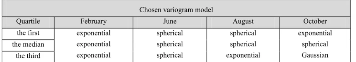
The summary of chosen variogram models for individual prediction cases is given in Table 2, all based on the minimal RMSE value of the estimated values.
Table 2. Chosen variogram models
Chosen variogram model
Quartile February June August October
the first the median
the third
exponential exponential exponential
spherical spherical spherical
spherical spherical exponential
Figure 2 shows the experimental variograms for all conducted predictions together with the corresponding (chosen) variogram models. What is evident is that the so-called hole effect, which points to a form of periodicity in the data, is present in almost every experimental variogram.
Figure 2. Experimental variograms with chosen variogram models for February, June, August and October 2009
variograms for whose calculation direction parameter was neglected (search area was a full circle).
The chosen variogram models were used in a prediction based on the indicator kriging method. Taking into consideration all of the above, one can draw a conclusion that the result of the application of this method aren't the desired maps of precipitation amount on the territory of the Republic of Serbia, but are rather probability maps of the occurrence of certain precipitation amount on the territory mentioned, for February, June, August and October 2009. If errors did not occur during the prediction procedure, all estimated probabilities would be in the range of [0,1] and would preserve the order of the thresholds used in prediction. However, errors inevitably occur, and therefore the estimated probabilities were corrected according to the procedure explained earlier in the paper. Firstly, all negative probability values were replaced with zero and all values greater than 1 with one. This ensured that all estimated values are within the permitted range of [0,1]. As far as preserving the order of probabilities is concerned, simple averaging of corresponding values was performed: e.g. in case that the estimated probability for a month at an observed location obtained from prediction in which the first quartile (q25) was used was greater than
the estimated probability obtained from prediction in which the median (q50) was used, both
values were substituted with their average value.
All calculations, as well as preparation of the final graphics, i.e. maps, was performed in the R open source software environment. R software solution offers lots of statistical and graphic tools within available R packages, together with a possibility of expanding and adjusting the environment to one's needs by creating new packages.
Figure 3 shows the maps of the estimated probabilities of the occurrence of a certain precipitation amount on the territory of the Republic of Serbia for distinctive months in 2009.
Three maps are given for each month: a left one uses the corresponding first quartile in the estimation procedure, a middle one for which the median was used and a right one in whose case the third quartile was used for the estimation procedure. The dark-grey colour corresponds to the interval [0.8,1], i.e. [80%,100%] and suggests that there is a great possibility that the monthly precipitation amount at an observed location doesn't exceed the threshold (the first quartile, the median or the third quartile). On the other hand, the white colour that corresponds to the interval [0,0.2] points to the fact that it's pretty unlikely the precipitation amount is within given limits, in other words it suggests that there is a huge possibility that the precipitation amount at an observed location exceeds the threshold value. By comparing three belonging maps for every month it is obvious that the area coloured with darker colours increases when going to the right. This means that as the threshold value increases (from the first to the third quartile) so does the probability of precipitation amount at a certain location being within the limits.
country receive more precipitation than the eastern ones, although they are located at the same latitude. The maps for February and October also suggest larger precipitation amounts in the central parts of Serbia.
Although the southwestern parts of Serbia generally tend to receive more precipitation, there are some areas like the Pešter plateau that feature unfavourable conditions for precipitation formation (left map and map in the middle for February in Figure 3). Anticyclones with cold and stable weather prevail in this region in winter, whereas descending air currents are common in summer. That is the reason why weather stations at Pešter receive less precipitation (700-800 mm) considering the elevation at which they are located.
Conclusion
Precipitation, as one of the most important climate variables, varies in space (and time). Simple mathematical functions cannot adequately describe those irregular variations and therefore more complex methods, including geostatistical interpolation methods, are required. These methods provide stochastic surfaces as a result and are used for that purpose. Within this paper, indicator kriging was used for describing spatial variations of precipitation on the territory of the Republic of Serbia, i.e. for their prediction.
The result of indicator kriging is a map of probabilities that depict variable values at observed locations. These variable values do not exceed a set boundary value given in advance, which was as such used during the transformation of the original data.
Maps of the probabilities of the occurrence of certain cumulative monthly precipitation amounts on the territory of the Republic of Serbia in February, June, August and October 2009 were created within the paper. Three maps were created for each month, using different threshold values (the first quartile, the median and the third quartile) for transformation of the original data values into indicators. The obtained maps correspond to the spatial distribution of precipitation in Serbia, thereby identifying the northern parts of the country, the Morava valley and Metohija as regions in which the occurrence of a smaller precipitation amount (the amount within the limits of the defined threshold) is more likely to happen. The western parts of Serbia feature greater probabilities of abundant precipitation occurrence, i.e. precipitation which by amount exceeds the limits defined when conducting prediction using the method of indicator kriging.
References
Atkinson, P. M. and Lloyd, C. D. (1998). Mapping Precipitation in Switzerland with Ordinary and Indicator Kriging. Journal of Geographic Information and Decision Analysis, Vol. 2, No. 2, p. 65-76.
Bajat, B. and Štrbac, D. (2003). Quality analysis of digital terrain models for the test area Zlatibor, Glasnik Srpskog geografskog društva, Vol. 83, No. 1, p. 31-42. (in Serbian)
Bajat, B. et al. (2013). Mapping average annual precipitation in Serbia (1961–1990) by using regression kriging. Theor Appl Climatol, 112(1), 1-13.
Bivand, R. S., Pebesma, E. J. and Gómez-Rubio, V. (2008). Applied Spatial Data Analysis with R. New York: Springer Science+Business Media, LLC.
Burrough, P. A. and McDonnell, R. A. (2006). Principles of Geographic Information Systems. Serbian translation by Bajat, B. and Blagojević, D., Beograd: Građevinski fakultet.
Ducić, V. and Radovanović, M. (2005). Klima Srbije, Beograd: Zavod za udžbenike i nastavna sredstva, str. 212. Glacken, I. and Blackney, P. (1998). A practitioners implementation of Indicator Kriging. Vann, J., ed. Proceedings
of the Symposium “Beyond Ordinary Kriging: Non-Linear Geostatistical Methods in Practice”. Perth: The Geostatistical Association of Australasia, p. 26-39.
Guimarães, R. J. P. S. et al. (2012). Use of Indicator Kriging to Investigate Schistosomiasis in Minas Gerais State, Brazil. Journal of Tropical Medicine [online], Vol. 2012. Available at:
http://www.readcube.com/articles/10.1155/2012/837428?locale=en [29.08.2013].
Isaaks, E. H. and Srivastava, R. M. (1989). Applied Geostatistics. New York: Oxford University Press.
Joksić, D. and Bajat, B. (2005). Probability maps as a measure of reliability for intervisibility analysis, SPATIUM, No. 12, p. 22-27.
Ј urnel, A. G. (1983). Nonparametric Estimation of Spatial Distributions. Mathematical Geology, Vol. 15, No. 3, p. 445-468.
Pejović, M., Bajat, B. and Luković, J. (2012). Spatial distribution of interpolation uncertainty: case study of isotherm map of Serbia (1991-2009). Glasnik Srpskog geografskog društva, Vol. 92, No. 4, p. 31-50. Republic Hydrometeorological Service of Serbia - RHMS (2013). Padavinski režim u Srbiji [online]. Available at:
http://www.hidmet.gov.rs/podaci/meteorologija/latin/Padavinski_rezim_u_Srbiji.pdf [10.08.2013].
Sun, X., Manton, M. J. and Ebert, E. E. (2003). Regional rainfall estimation using double-kriging of raingauge and satellite observations. BMRC Research Report No. 94. Melbourne: Australian Government, Bureau of Meteorology.
Tolosana-Delgado, R. (2007): Simplicial Indicator Kriging: presentation [online]. Wuhan: China University of Geosciences. Available at: http://www.sediment.uni-goettingen.de/staff/tolosana/extra/Wuhan-talk-4.pdf [21.08.2013].
Unkašević, M. and Tošić, I. (2011). A statistical analysis of the daily precipitation over Serbia: trends and indices. Theoretical and Applied Climatology, 106:69–78.
Ј Ш Х
Ј Ј
Ј Ћ2
, Ј 1
,Ј Ћ2
1У а – Г ађ а , О а а , а а а
а а 73, 11000 а
2У а – Г а а , С 3/3, 11000 а
:
2009. . ђ
ђ
.
: , ,
,
ђ , ,
.
(Burrough and McDonnell, 2006).
.
. Ј : (Zhang, 2011).
( . Best Linear Unbiased Estimate -
BLUE) ђ .
,
. , (
) ,
ђ ђ (Pejović et al., 2012).
,
, , .
(Bajat et al., 2013). , ,
ђ
2009. , (
)
. ђ
, (Joksić and
Bajat, 2005).
:
. ,
, .
,
, , (RHMS, 2013).
, ,
2
47014, T 36009 43007
ђ , ,
2009. .
,
, (Burrough and
McDonnell, 2006):
( )
x
=
m
( )
x
+
ε
'
( )
x
+
ε
"
Z
(1):
( )
x
Z
- ,( )
x
m
- . , . ,( )
x
'
ε
- ( ), ,
"
ε
- , . ., , ( ) , : , , , , , , . , . . , , , ( ) , . ( . threshold).
( . Journel) 1983.
, ,
.
, ,
(Tolosana-Delgado, 2007), (Atkinson and Lloyd, 1998; Sun et
al., 2003), ,
( а . schistosomiasis) (Guimarães et al., 2012).
, . .
( ) ,
1 0,
(Isaaks and Srivastava, 1989).
, :
(
)
( )
( )
⎩
⎨
⎧
>
≤
=
k k kz
x
z
z
x
z
z
x
i
,
0
,
1
,
(2) :( )
x
z
-x
,k
z
- , . ,(
x
z
ki
,
)
- ( )x
,.
k
,
(Glacken and Blackney, 1998).
( . conditional cumulative distribution function - ccdf), .
( )
. , ,
,
( . 5.2 mg, 106 mm .) ,
( )
.
.
. , ( ),
, .
ђ (Burrough and McDonnell,
2006).
. :
( )
∑
[
( ) (
)
=
+
−
=
ni
i
i
z
x
h
x
z
n
h
1
2
2
1
ˆ
γ
]
(3), ђ
.
, . ( . fit)
.
n
z
h
, ,
.
.
( . sill) (Burrough and
McDonnell, 2006).
ђ ,
, ,
.
, „ “ ( . nested), .
(Burrough and McDonnell, 2006).
( ) ђ
.
, . , , .
, . ђ ,
, . ђ
,
.
, , ,
, . ,
(Isaaks and Srivastava, 1989). ,
.
, .
( ) ,
[0,1]. ђ ,
, . ,
( .
,
). ђ ,
, „ “ : ,
ђ 100%,
. ( . order relation violations)
ђ ђ .
ђ
, 1 .
[0,1].
(
), ђ .
( )
, ,
(Isaaks and Srivastava, 1989).
( ) (Atkinson and Lloyd, 1998),
,
. , ,
( ) .
( , , . „ “ .)
.
( ),
.
ђ , qq-plot-
.
ђ
2009. .
, (RHMS, 2013), ,
. ђ ,
,
.
ђ .
, ,
, , 2009. .
191 . ,
1 km x 1 km (
).
,
.
, qq-plot- - . ђ
( , , , 2009.
) ђ .
, 2009.
( 1) ( . positively skewed),
.
1. Х , , 2009.
, . -
1 0.
.
2009. ,
, , .
, q25 ( 25% ,
, , , ),
q50 ( 50% ),
q75 ( 75% ) (
1).
,
ђ . ђ
, ,
- .
. ,
( )
ђ .
( . Root Mean Squared Error - RMSE) (Bajat and Štrbac, 2003).
1.
2
, .
2.
2
( ) .
. ( . hole effect)
.
2. , ,
2009.
( ) ,
ђ ( - , - ,
, ђ
( ).
. ,
,
ђ ,
, , 2009. .
, [0,1]
. ђ , ,
.
, 1 .
ђ [0,1].
, : .
(q25)
(q50), .
, , . ,
R open source . R
R
( . packages), ђ
.
3 ђ
2009. .
:
,
. [0.8,1], . [80%,100%],
( , ).
, [0,0.2]
, ,
. ,
.
( )
.
.
,
(Ducić and Radovanović, 2005), ђ 3 (
, ).
. ,
( 3). ђ ,
,
.
( ).
(Unkašević and Tošić, 2011).
, .
ђ
.
3. ђ
, ,
( 3).
ђ ,
.
(700-800 mm) .
, ,
( ). Ј
, ,
.
, , .
, .
( )
.
ђ
, , 2009. .
, ( ,
) .
,
,
( ).
, .
ђ
.
ђ
. ,
, ,
ђ . ђ
( , , .)