Rainfall Depth-Duration-Frequency Relationships for South Carolina, North Carolina, and Georgia

ISSN 1553-345X

© 2007 Science Publications

Corresponding Author: A. A. Khan, 218 Lowry Hall, Department of Civil Engineering, Clemson University, Clemson, SC, 29634-0911, USA, Tel: 864-656 3327, Fax: 864-656 2670

Rainfall Depth-Duration-Frequency Relationships for South Carolina, North Carolina, and

Georgia

J. P. Raiford, N. M. Aziz, A. A. Khanand D. N. Powell Department of Civil Engineering, Clemson University,

Clemson, SC, 29634-0911, USA

Abstract: The depth-duration-frequency curves and isopluvial maps for the region encompassing South Carolina, North Carolina, and Georgia were developed using the available rainfall data. The aim was to update the existing intensity-duration-frequency curves in the region and obtain these curves at ungauged sites throughout the region using the newly developed rainfall frequency analysis techniques. A total of 17 durations ranging from 15 minutes to 120 hours for return periods of 2, 10, 25, 50, and 100 years were analyzed. The L-moment method with X-10 test was used to search for homogeneous regions within the study area. It was found that the method was either unable to homogeneous regions that were geographically contiguous or too many stations had to be eliminated before a region could be considered homogenous. Finally, at-site statistics were calculated to develop frequency relationships. Normal, lognormal, generalized extreme value, Pearson type III, and log Pearson type III probability distribution functions were used to fit the maximum annual precipitation data at each gauging site for each duration. The chi-squared goodness-of-fit test was used to determine the best fit probability distribution. The new intensity-duration-frequency curves were found to be lower than the existing curves developed in 1986. The difference between the two set of curves was found to be due to the removal of the outliers in the present study and the existence of the post 1986 drought conditions in the region. The spatial interpolation of the rainfall intensity from the depth-duration-frequency curves was found to yield accurate intensity-depth-duration-frequency curves and could be used to develop these curves at ungauged sites in the study area.

Keywords: Maximum annual precipitation, intensity-duration-frequency curves, isopluvial maps INTRODUCTION

Rainfall is an integral component in the hydrologic cycle. Engineers must be able to quantify rainfall in order to design structures impacted by or dealing with the collection, conveyance, and storage of excess rainfall. Quantification of rainfall is generally done using isopluvial maps and intensity-duration-frequency (IDF) curves. These two tools are used by engineers to design safe and cost efficient structures for certain return periods, thus accepting a certain amount of risk that the capacity may be exceeded.

In the last fifty years, new rainfall frequency analysis techniques have been developed. Many government agencies are beginning to make use of these new techniques to update their depth-duration-frequency (DDF) relationships. It has been suggested that DDF estimates be updated every 20 years[5]. DDF relationships for South Carolina were last updated in 1988[10]. Updating these relationships every 20 years not only increases the record length of the data set, allowing for more accurate prediction of larger return periods, but also allows new rainfall gauging stations to be included. The aim of this study is to collect the rainfall data from South Carolina, North Carolina, and Georgia and analyze it using recently developed methods.

A recent method for estimating the parameters of a probability distribution (such as mean, standard deviation, etc.) is the L-moment method. This method uses linear combinations of order statistics to estimate population values. The bias of these sample statistics is small for small samples and less dependent on any one distribution. Also, if the bias does exist, it is not compounded by squaring or cubing each observation because the L-moment sample statistics are linear[4]. Another development in analyzing rainfall data is the identification of homogenous regions. Several researchers have developed methods for determining homogenous regions, for example, Dalrymple[1], Whiltshire[16], Hosking[3], and Lu and Stedinger[7]. A homogenous region is a group of sites that can be described by the same statistical distribution. The probability distribution at all sites is expected to have the same coefficient of variation and skew. The best fit distribution for the whole region is determined using moment diagrams, growth curves, or bias testing.

L-moment method with the maximum likelihood method and log-log graphical analysis for ten states in the Midwest and found the maximum likelihood method to be the least conservative and L-moments to be the most conservative. Naghavi and Yu[8] used L-moments and defined three homogenous regions based on AMP and selected a generalized extreme value distribution for extreme events in Louisiana. Parrett[9] attempted to divide stations based on maximum annual precipitation (MAP) and elevation differences, however, both methods failed to produce acceptable regions. L-moments have also been used in studies in Montana[9], the Ohio River Basin[6], Oklahoma[14], and Colorado[13].

In this study, IDF curves and isopluvial maps are developed for 17 different durations (ranging from 15 minutes to 120 hours) and 5 different return periods in a region that includes South Carolina, North Carolina, and Georgia. Data collection and verification is the first step in the process. Maximum annual precipitation is obtained for the selected durations at each station and corrected to account for the difference in maximum precipitation within the duration and recording intervals based on clock time. Next, an appropriate frequency distribution is obtained at each station for the selected durations. Finally, spatial analysis is performed to interpolate rainfall values between stations on the map and regression analysis is performed to interpolate rainfall values between durations on an IDF curve. The impact of outliers and the length of record on the final IDF curves are assessed. The development of homogenous regions is also explored.

DATA COLLECTION AND VERIFICATION

Rainfall data was obtained from two sources. The first was the Southeastern Regional Climate Center (SERCC) and the second source was EarthInfo, a commercial source. At some stations data was available for more than one period, e.g., hourly and daily, 15-minute and daily, or all three types. All of the raw data required verification and quality control.

The daily data has the longest record of the three data types with records at some of the stations beginning as early as 1889. For all three periods, the data files were reformatted to show continuous data from the start date, ensuring continuity of the rainfall data and providing an easy way to compare rainfall data across stations.

Some missing rainfall values in the daily rainfall data files could be estimated using the normal ratio method. The annual mean precipitation (AMP) values were calculated for each of the daily stations and a missing value, if present, was interpolated from the three closest sites within a 10-mile radius. If three sites were not available, the missing flag remained in place. Also, if two out of the three closest stations had a zero rain value on that day, the missing value was assumed to be zero. While the method did allow for some rainfall values to be interpolated, the criteria mostly inferred that no rainfall occurred during missing

periods. Due to the low density of hourly and 15-minute stations, the normal ratio method could not be used to interpolate missing data. The hourly and 15-minute data contained accumulated rainfall values. These values were evenly divided over the accumulated periods.

MAXIMUM ANNUAL PRECIPITATION SERIES

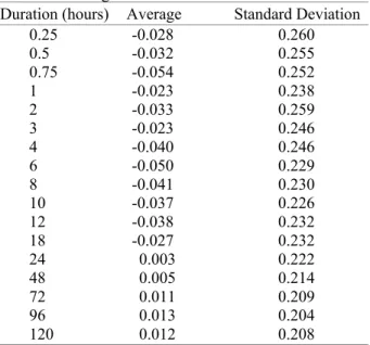
The maximum annual precipitation (MAP) series was extracted by a running-sum method from each site. Durations of 0.25, 0.5, 0.45, 1, 2, 3, 4, 6, 8, 10, 12, 18, 24, 48, 72, 96, and 120 hours were considered in this study. The number of MAP series at a particular station would depend on the recording interval, for example, a daily rainfall recording station would have 5 MAP series. Each MAP series was fitted to a normal distribution and values outside of a 98 percent confidence interval were considered outliers. Some stations had both 15-minute and hourly data, in this case two data sets were available for a few durations, however, the larger of the two MAP values was used in the analysis.

Table 1: Average serial correlation

Duration (hours) Average Standard Deviation

0.25 -0.028 0.260

0.5 -0.032 0.255

0.75 -0.054 0.252

1 -0.023 0.238

2 -0.033 0.259

3 -0.023 0.246

4 -0.040 0.246

6 -0.050 0.229

8 -0.041 0.230

10 -0.037 0.226

12 -0.038 0.232

18 -0.027 0.232

24 0.003 0.222

48 0.005 0.214

72 0.011 0.209

96 0.013 0.204

120 0.012 0.208

and the maximum value is 0.95. This shows an absence of a linear trend in the data and hence no significant correlation of the data across the stations.

SCALE CORRECTION FACTORS

Since rain gauge stations record at clock hour intervals, rainfall maxima may overlap the recording times. At a daily site, there is a greater chance of missing 24-hour duration maximum rainfall due to these overlaps than at a 15-minute site aggregated for the same duration. In order to compare maxima from different sites that may have different recording intervals, a scale correction factor (SCF) must be applied to the data. Hershfield[2] developed a relationship between 60-minute rainfall data and fixed clock hour data and found the ratio to be 1.13. The same ratio was found for daily data. Young and McEnroe[17] confirmed these ratios and developed a general equation for SCF as given below

1.5 1 0.13 t

SCF

D

∆  

= + _{ }

  (1)

where SCF is the scale correction factor, ∆t is the observation time step at a rain gauge site, and D is the duration under investigation. In this study, Eq. (2) is used to determine SCF for the MAP series of the selected durations based on the recording time interval of the station.

FITTING PROBABILITY DISTRIBUTION TO THE MAP SERIES

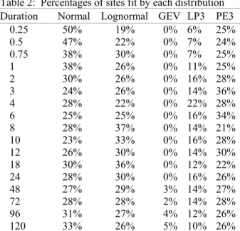
The MAP series for the selected durations at each station was fitted to five different probability distributions. The probability distributions selected for this study were normal, lognormal, generalize extreme value, Pearson type III, and log Pearson type III. The best fit was determined based on the chi-squared goodness-of-fit test. The critical chi-squared value of each distribution was compared to the limiting value (based on number of bins, number of parameters of the fitted probability distribution, and the confidence interval) to select the best distribution for that duration at that site. Table 2 shows the percentage of sites that were best fit by each distribution for various durations (in hours).

It is generally accepted that data should not be extrapolated more than twice the record length. Sites with smaller record lengths may be used in predicting

smaller return period values. The maximum available record length for a 15-minute MAP series is only 32 years. In this study, only the stations with 10 or more years of data were used. For return periods of less than or equal to 25 years, the rule of twice the record length was applied. For return periods greater than 25 years, only stations with at least 20 years of record length were used.

Table 2: Percentages of sites fit by each distribution Duration Normal Lognormal GEV LP3 PE3

0.25 50% 19% 0% 6% 25%

0.5 47% 22% 0% 7% 24%

0.75 38% 30% 0% 7% 25%

1 38% 26% 0% 11% 25%

2 30% 26% 0% 16% 28%

3 24% 26% 0% 14% 36%

4 28% 22% 0% 22% 28%

6 25% 25% 0% 16% 34%

8 28% 37% 0% 14% 21%

10 23% 33% 0% 16% 28%

12 26% 30% 0% 14% 30%

18 30% 36% 0% 12% 22%

24 28% 30% 0% 16% 26%

48 27% 29% 3% 14% 27%

72 28% 28% 2% 14% 28%

96 31% 27% 4% 12% 26%

120 33% 26% 5% 10% 26%

IDENTIFICATION OF HOMOGENEOUS REGIONS

The identification of homogeneous regions is a critical step in regional analysis. To identify homogenous regions in this study, the X-10 test developed by Lu and Stedinger[7] is used. The first step is to calculate L-moments for the ordered (from smallest to largest) and ranked MAP series at each site for each duration. Using the L-moment statistics, the MAP series is fitted to a generalized extreme value distribution with a mean of 1.0, and a 10-year return period rainfall at site j is determined as follows

( )

(

)

(

)

(

)

( )

( )

2 0.9

2

3

ln 0.9

1 1

1 1 2

7.859 2.9554

ln 2 2

3 ln 3

j

C C

C

ψ

ψ

τ ξ

ψ

ψ

τ

−



 ₋ 



 

= + _ − _

Γ +

− _{ }

 



= + 

 

= −

 +

 

where ξ_0.9j is the 10-year return period rainfall event at station j, Γ is the gamma distribution, ψ is the shape parameter of the distribution, and τ₂, τ₃ are L-moment statistics. The regional 10-year return-period rainfall,

0.9R

ξ , is calculated using a record length weighted average site’s rainfall and is given below

0.9 1 0.9

1

N j j j R

N j j

n

n ξ

ξ =

=

=

∑

∑

(3)

where N is the number of stations in the region that is tested for homogeneity and n is the number of data in the MAP series at station j. The critical chi-squared value is calculated using the following equation

(

)

( )

2 0.9 0.9 2

1 _0.9

j R

N

R _j

j Var

ξ ξ

χ

ξ

=

−

=

_∑

where χ2_R is the critical chi-squared regional value,

( )

Var ξ is the 10-year return period asymptotic variance. The 10-year asymptotic variance values, based on the coefficient of variation and kurtosis, are tabulated by Lu and Stedinger[7]. Correction factors for the asymptotic variance are also provided by the above authors. The correction factors are functions of sample size, coefficient of variation, and kurtosis. In order for a region to be considered homogeneous, the critical chi-squared value must be less than the limiting chi-chi-squared value. The limiting chi-squared value is determined based on a confidence interval (0.05) and degrees of freedom

(

)

Three procedures were attempted to obtain homogeneous regions. The first was a jackknife method, where all the sites were tested as a region. If the test failed, the site with the largest chi-squared value was removed and the remaining sites were tested. When a region was found, the sites that formed the region were removed and the remaining sites were tested in the same manner until all the sites were included in a region. Seventeen regions were found, however, the sites were spread out over the three states. The results can be seen in Fig. 1. Similar symbols show site locations that form a region. Although homogeneous regions were found, the regions did not show geographic coherence.

The second procedure was a graphical approach. All the data at a station for a particular duration was fitted to a GEV distribution using L-moments and sites that had curves with similar shapes were grouped into a region. Only one region was identified and contained only 7 sites.

-84 -82 -80 -78 -76

Longitude (degrees)

32 34 36

La

tt

it

u

d

e (

d

eg

rees

)

Fig. 1: Regions identified by jackknife method

-85 -84 -83 -82 -81 -80 -79 -78 -77 -76 -75

Longitude (degrees)

30 31 32 33 34 35 36 37

La

tt

it

u

d

e (

d

egre

es)

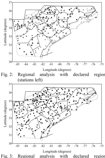
Fig. 2: Regional analysis with declared region (stations left)

-85 -84 -83 -82 -81 -80 -79 -78 -77 -76 -75

Longitude (degrees)

30 31 32 33 34 35 36 37

La

tt

it

u

d

e (

d

egre

es)

The third method was a variation of the first. To ensure that the homogeneous regions identified were geographically contiguous, regions were declared and then tested for homogeneity. If a region failed homogeneity test, a site was removed using the jackknife method described above until a homogeneous region was obtained. Fig. 2 shows the final delineation of the regions with sites that remained. Fig. 3 shows the regions with sites removed during the process. In most cases more than half the sites had to be removed before a regional solution could be found, so it was obvious that the scheme would not yield satisfactory results.

ISOPLUVIAL MAPS

After fitting the MAP series at each site for the selected durations with a best fit probability distribution, the rainfall depths for each return period were then extracted from that probability distribution. Using a 0.5-degree latitude by 0.5-degree longitude grid, DDF values at the grid points were interpolated by the Kriging method. These values were used to draw isopluvial maps for a given duration over the whole region. An example of such a map is shown in Fig. 4. Complete details are provided by Raiford[11].

-84 -82 -80 -78 -76

Longitude (degrees)

32 34 36

Latitude (degree

s)

Fig. 4: Typical Isopluvial Map (15-Minute, 2-Year) IDF CURVES

Using the DDF values at a site, the IDF curves were generated using the equation below

(

)

s

t

cT i

d D =

+ (5)

where

i

are curve parameters. The above form of the equation for IDF curves is identical to that proposed by Wanielista et al.[15] Rainfall intensities for the five minutes duration were also extrapolated from the fitted

curve. The regression coefficients for all the fits were above 0.98. A typical IDF curve at Columbia, South Carolina is shown in Fig. 5.

Comparisons of the existing IDF relationships to those produced in this research for the cities of Greenville and Columbia in South Carolina showed that the existing IDF values were higher than those produced in this study. However, the agreement between the new and existing data improved as duration increased. In order to identify the reasons for the differences between the existing curves and those produced in this research, three tests were performed and the results were compared for the two cities.

0.01 0.1 1 10

0.1 1 10 100

Duration (hours)

Int

ensi

ty

(

inc

hes/

hour)

2-yr 10-yr 25-yr 50-yr 100-yr Existing (2-yr) Existing (10-yr) Existing (25-yr) Existing (50-yr) Existing (100-yr)

Fig. 5: Typical IDF curve for Columbia, South Carolina, with outliers removed

The first test was intended to identify the impact of removing outliers from the data sets. For this purpose, IDF relationships were generated from the data at an individual gauging station near the city of interest without removing the outliers. The comparisons of these IDF curves with the existing curves are shown in Figs. 6 and 7. The results indicate that the difference in IDF values with the outliers were smaller than those presented in the previous section without the outliers.

0.01 0.1 1 10

0.1 1 Duration (hours) 10 100

Int

ensi

ty

(

inche

s/

hour

)

2-yr 10-yr 25-yr 50-yr 100-yr Existing (2-yr) Existing (10-yr) Existing (25-yr) Existing (50-yr) Existing (100-yr)

0.01 0.1 1 10

0.1 1 _{Duration (hours)} 10 100

Int

ensi

ty

(i

nches/

hour)

2-yr 10-yr 25-yr 50-yr 100-yr Existing (2-yr) Existing (10-yr) Existing (25-yr) Existing (50-yr) Existing (100-yr)

Fig. 7: Effect of outliers on IDF values in Columbia, South Carolina

The second test examined the effects of new data by only using data that was available when the existing curves were published[10]. The publication did not include information about outlier removal. Therefore, the test was performed using data recorded before 1986 and without removing any outliers in the data. The comparison of these IDF curves to current curves show good agreement as seen in Figs. 8 and 9. However, since it is not clear what stations were used in the development of the existing curves, it was not possible to clearly duplicate previous work and reach a very definite conclusion.

0.01 0.1 1 10

0.1 1 Duration (hours) 10 100

In

te

nsit

y

(

inch

es/hou

r)

2-yr 10-yr 25-yr 50-yr 100-yr Existing (2-yr) Existing (10-yr) Existing (25-yr) Existing (50-yr) Existing (100-yr)

Fig. 8: Effect of Post 1986 Data on IDF Values in Greenville, South Carolina

0.01 0.1 1 10

0.1 1 _{Duration (hours)} 10 100

Int

ensi

ty

(

inc

hes/

hour) 2-yr

10-yr 25-yr 50-yr 100-yr Existing (2-yr) Existing (10-yr) Existing (25-yr) Existing (50-yr) Existing (100-yr)

Fig. 9: Effect of Post 1986 Data on IDF Values in Columbia, South Carolina

0.01 0.1 1 10

0.1 1 _{Duration (hours)} 10 100

In

te

nsi

ty

(i

nches/

hour

)

2-yr 10-yr 25-yr 50-yr 100-yr Spatial Analysis (2-yr) Spatial Analysis (10-yr) Spatial Analysis (25-yr) Spatial Analysis (50-yr) Spatial Analysis (100-yr)

Fig. 10: Effect of Spatial Analysis on IDF Values in Greenville, South Carolina

0.01 0.1 1 10

0.1 1 _{Duration (hours)} 10 100

In

te

ns

it

y

(

inc

hes/

hour

)

2-yr 10-yr 25-yr 50-yr 100-yr Spatial Analysis (2-yr) Spatial Analysis (10-yr) Spatial Analysis (25-yr)

Fig. 11: Effect of Spatial Analysis on IDF Values in Columbia, South Carolina

The third test examined the effects of the spatial analysis on the new curves. This was accomplished by generating IDF relationships at a specific gauging station and comparing the results with the spatially analyzed IDF curves. The comparison is shown in Figs. 10 and 11 and indicates a good agreement. This implies that the spatial analysis may be used to obtain IDF curves at ungauged sites.

CONCLUSIONS

In this study, the product moment method and the L-moment method with regional analysis were investigated for developing iospluvial maps and IDF curves in South Carolina, North Carolina, and Georgia. The L-moment method with X-10 test was used to search for homogeneous regions within the study area. The method used was either unable to identify geographically contiguous regions or too many stations had to be eliminated before a declared region could be deemed homogeneous.

value, Pearson type III, and log Pearson type III distributions for each duration. The distribution selected based on the chi-squared test was then used to find depth-duration-frequency (DDF) values at 2, 10, 25, 50, and 100 years. These DDF values were spatially interpolated to obtain isopluvial maps for all durations and return periods. Comparison of IDF values determined from the rainfall data at a specific station to the spatially interpolated values at the same location revealed no significant difference. This proved that the IDF curves can be obtained from the isopluvial maps at ungauged sites.

The computed IDF curves were compared with the existing curves at the selected sites. The computed IDF curves were found to be lower than the existing IDF curves. The removal of outliers was found to have significant impact on the magnitude of IDF values. The drought conditions in the study area also contributed to the lower IDF value as suggested by the pre and post 1986 rainfall frequency analysis.

ACKNOWLEDGMENTS

The financial support for this project was provided by the South Carolina Department of Transportation through a grant to the Civil Engineering Department at Clemson University.

REFERENCES

1. Dalrymple, T., 2004. Flood frequency analyses. Geological Survey Water-Supply Paper 1543-A, Washington.

2. Hershfield, D.M., 1961. Rainfall frequency atlas of the United States. Weather Bureau Technical Paper 40, U.S. Department of Commerce.

3. Hosking, J.R.M., 1992. Moments or L-moments? An example comparing two measures of distributional shape. The American Statistician, 46(3): 186-189.

4. Hosking, J.R.M. and J.R. Wallis, 1997. Regional Frequency Analysis: An Approach Based on L-moments,” 1st Ed., Cambridge University Press, Cambridge, U.K., pp: 224.

5. Huff, F.A. and J.R. Angel, 1992. Rainfall frequency atlas of the Midwest. Illinois State Water Survey Bulletin 71.

6. Julian, L.T., B. Lin, J.M. Daniel, T. Davila, E.H. Chin, S.M. Gillette and M. Yekta, 1997. Ohio River Basin precipitation frequency study. PR. 1-13, Office of Hydrology, NWS, Silver Spring, Maryland.

7. Lu, L.H. and J.R. Stedinger, 1992. Sampling variance of normalized GEV/PWM quantile estimators and a regional homogeneity test. Journal of Hydrology, 138: 223-245.

8. Naghavi, B. and F.X. Yu, 1995. Regional frequency analysis of extreme precipitation in Louisiana. Journal of Hydraulic Engineering, ASCE, 121(11): 819-827.

9. Parrett, C., 1997. Regional analysis of annual precipitation maxima in Montana. Water-Resources Investigations Report 97-4004, USGS. 10. Purvis, J.C., W. Tyler and S. Sidlow, 1988.

Maximum rainfall intensity in South Carolina by county. Climate Report No. G32, South Carolina State Climatology Office. Columbia, SC.

11. Raiford, J.P., 2004. Rainfall depth-duration-frequency relationships for NC, SC, and GA. Master Thesis, Clemson University, Clemson, SC, pp: 213.

12. Schaefer, M.G., 1990. Regional analyses of precipitation annual maxima in Washington State. Water Resources Research, 26(1): 119-131.

13. Sveinsson, O.G.B., J.D. Salas and D.C. Boes, D. C., 2002. Regional frequency analysis of extreme precipitation in Northeastern Colorado and Fort Collins flood of 1997. Journal of Hydrologic Engineering, 7(1): 49-63.

14. Tortorelli, R.L., A. Rea and W.H. Asquith, 1999. Depth-duration-frequency of precipitation for Oklahoma. Water-Resources Investigations Report 99-4232, USGS.

15. Wanielista, M., R. Eaglin and E. Eaglin, 1996. Intensity-duration-frequency curves for the State of Florida. Florida Department of Transportation. 16. Whiltshire, S.E. 1986. Regional flood frequency

analysis I: Homogeneity statistics. Hydrological Sciences Journal, 31(3): 321-333.

17. Young, C.B. and B.M. McEnroe, 2002. Precipitation frequency estimates for the Kansas City metropolitan area. Sponsored by Kansas City Metro Chapter of American Public Works Association, University of Kansas.