Aerodynamic Forces with Local Dynamics on Rotor
Blade under Unsteady Wind Inflow
MUHAMMAD RAMZAN LUHUR*, JOACHIM PEINKE**, AND MATTHIAS WAECHTER*** RECEIVED ON 17.05.2013 ACCEPTED ON 11.09.2013
ABSTRACT
This contribution provides the development of a stochastic lift and drag model for an airfoil FX 79-W-151A under unsteady wind inflow based on wind tunnel measurements. Here we present the integration of the stochastic model into a well-known standard BEM (Blade Element Momentum) model to obtain the corresponding aerodynamic forces on a rotating blade element. The stochastic model is integrated as an alternative to static tabulated data used by classical BEM. The results show that in comparison to classical BEM, the BEM with stochastic approach additionally reflects the local force dynamics and therefore provides more information on aerodynamic forces that can be used by wind turbine simulation codes.
Keywords: Wind Tunnel Measurements, Unsteady Wind Inflow, Stochastic Model, Lift Dynamics, Drag Dynamics, Blade Element Momentum Method, Local Force Dynamics.
*Ph.D. Researcher, **Professor, and ***Post-Doctoral Researcher, ForWind-Centre for Wind Energy Research, University of Oldenburg, Germany.
1.
INTRODUCTION
T
he dynamic nature of the wind contributes to the complex operation of wind turbines being exposed to turbulent atmospheric air flows having well-known complex statistics and gusty behavior [1-3]. The operation of wind turbines in such environment leads to several risks especially in terms of highly dynamic mechanical loads [4-5]. Several studies exist on placing an airfoil into a steady low-turbulence inflow and observing the lift and drag properties at constant AOAs (Angles of Attack) [6-9], however, the complexity of open-air turbulent flows is yet to be perceived fully.The blade aerodynamics under turbulent wind conditions changes profoundly compared to steady low-turbulence
flows. In unsteady flow the fast variations in AOA can lead to well-known dynamic stall effect resulting in significant increase in lift dynamics, compare [10-12].
To estimate the aerodynamic forces on wind turbine rotor
blades several engineering and CFD (Computational Fluid
Dynamics) techniques exist today [1,13-16]. However, from
performance point of view still engineering methods are
the leading choice over CFD [17]. CFD yet needs more
powerful computers to achieve acceptable computational
time [18]. Still most wind turbine aerodynamic computations
are performed with standard BEM method due to its
Mehran University Research Journal of Engineering & Technology, Volume 33, No. 1, January, 2014 [ISSN 0254-7821]
Nevertheless, most of the aerodynamic models use
tabulated static data for an airfoil at constant AOAs
[19-20] to estimate the forces on wind turbine blades, and
therefore lack the information on the local dynamics.
In this work, a stochastic model of the lift and drag
dynamics is integrated into a classical BEM as an
alternative to static airfoil data table to obtain the
aerodynamic forces with complete local dynamics. The
model evaluates the lift and drag forces numerically as
function of AOA. The forces are obtained for a rotating
blade element and are compared with results obtained with
classical BEM (with the use of static airfoil data table).
The model is being developed to extract and provide the
detailed local loading information acting on the wind
turbine blades which could lead to an optimum rotor design
under turbulent wind conditions. The final goal is to
achieve an aerodynamic model like AeroDyn [19] based
on stochastic approach. Later it could be combined with a
wind energy converter model to obtain a stochastic rotor
model.
The paper is structured as follows. Section 2 describes
the lift and drag modeling approach. Section 3 explains
the calculation of rotor normal and tangential forces for a
blade element in the context of classical and stochastic
BEM (with model addition) methods. Section 4 presents
the results from both the classical and the stochastic BEM
approaches. Finally section 5 concludes the outcome.
2.
STOCHASTIC LIFT AND DRAG
MODEL
The stochastic modeling of lift and drag dynamics is
consisting of two steps. First, measurements have been
performed in wind tunnel to obtain the airfoil data. Second,
a stochastic approach is applied with an optimization
scheme to model the lift and drag dynamics.
2.1
Measurements
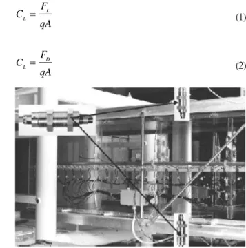
The measurements have been performed in a closed loop
wind tunnel of Oldenburg University for an airfoil FX
79-W-151A having chord length of 0.2m. The wind tunnel
has a test section of 1m wide, 0.8m high and 3m long. The
turbulent inflow was generated using a fractal square grid
having closer characteristics to natural wind [21-22]. The
lift and drag forces were measured directly using two strain
gauge force sensors fixed at the end points of an airfoil in
span-wise direction as shown in Fig. 1. The mean wind
velocity and Reynolds number were 50m/s and 7x10⁵
respectively. Further details of the measurement can be
found in [22].
2.2
Stochastic Modeling
The lift and drag coefficients are modeled using a stochastic
approach which extracts most of the information available
in the system dynamics. First, lift and drag coefficients are
calculated from measured data using the relations [22]:
qA F
C L
L = (1)
qA F
C D
L = (2)
FIG. 1. VIEW OF THE WIND TUNNEL TEST SECTION. BLACK ARROWS SHOW THE POSITION OF FORCE SENSORS
Where FL is the lift force, FD the drag force, q the inflow dynamic pressure and A the area of the airfoil.
The stochastic approach is applied on the measured time
series of lift and drag coefficients using a first order
stochastic differential equation called the Langevin
equation, cf. [23]. The approach is based on drift and
diffusion functions coupled with a noise term. It models
the complex statistics by means of random numbers. The
approach reads: ) ( . ) ( ) 2 ( ) ( ) 1 ( ) ( t X D X D dt t dX Γ + = (3)
Where Γ(t) is a Gaussian white noise termed as Langevin force [23] with mean value of
〈
Γ(t)〉
=0 and variance〈
Γ2(t)〉
=2. It is an uncorrelated statistical noise obeying the PDF (Probability Density Function) of normaldistribution.
The D(1)(X) and D(2)(X) are the drift and diffusion functions, also known as first and second Kramers-Moyal
coefficients for X(t). The drift and diffusion functions can be estimated from measured time series using the relation
[24-26]:
(
τ)
ατ α
τ ! ( ) () () ,
1 lim ) , ( 0 2 , 1 ) 1 ( X t X t X t X n n X
D = + − n =
→
= (4)
Where X represents the lift and drag coefficients, α the fix AOA, D(1)(X,α) the drift function and D(2)(X,α) the diffusion function. The drift function represents
the deterministic part of the system and estimates the
mean time derivative of the X(t) whereas the diffusion function quantifies the amplitude of the stochastic
fluctuations.
The direct estimation of D(1)(X,α) and D(2)(X,α) from Equation (4) may suffer from different sources of errors
like finite sampling deviations, additional measurement
noise etc. [22-28]. The Langevin Equation (3) is mainly
dependent on these two functions which means quality
of results strongly depend on the correct estimation of
drift and diffusion functions. For this purpose, an
optimization approach based on χ2 test is applied on PDFs
of the model and measured data. The χ2 value is obtained
as:
(
)
(
)
∑ = i − Measure,i Model,i p p+ Measurei
i
Model p
p , ,
2
2
χ (5)
Where pModel and pMeasure are the stationary PDFs of model and measured data respectively. The χ2 test quantifies the
difference between the model and measured data sets.
The lower the difference the better the quality of the results.
Since the Langevin Equation (3) is random by nature due
to involvement of the noise term, so it would be
time-consuming to get the stable values by numerical
simulation. As an alternative, the stationary PDF of the
Langevin equation is used, which is known in its analytical
form [23]:
(
X
Model)
( )
y
dy
( )
y⎥⎦
⎤
⎢⎣
⎡
∫= XModel
D D N
p (2)
) 1 (
(
X
Model)
D(2) exp (6)
Where N is a normalization factor.
For best estimation of drift and diffusion functions in
an automatic way, the optimization approach described
in Equation (5) is coupled with an interval sectioning
procedure based on the Inverse Parabolic Interpolation
algorithm [28]. The analytical expression for the
algorithm is:
[
]
[
]
[
() ()]
( )[
() ( )]
) ( ) ( ) ( ) ( ) ( ) ( ) ( 21 2 2
Mehran University Research Journal of Engineering & Technology, Volume 33, No. 1, January, 2014 [ISSN 0254-7821]
Where x is the abscissa value of new estimated point and accounts for diffusion function here. The
corresponding ordinate value of this new point is the χ2 value. The a, b, and c are the abscissa values of the three randomly selected points and f(a), f(b) and f(c) are the respective ordinate values of the three points along the inverse parabolic line. The algorithm works in a way that
it discards one point after each iteration and decides for a new set of three points for next iteration like the point with minimum ordinate value is always in the middle of
the three points. The algorithm continues for several iterations until the best value for x is obtained and thereafter stops functioning automatically as the points coincide with each other.
The basic model (Equation (3)) has been extended to incorporate for additional effects to reproduce satisfactory conditional PDFs p(X(t+τ) X(t)) for all time lags τ. These additional effects include out of phase lift and drag coefficients oscillation and the amplitude modulation
(breathing) observed in the lift and drag coefficients time series. The extended model reads [29]:
⎥
⎥
⎥
⎦
⎤
⎢
⎢
⎢
⎣
⎡
⎟
⎠
⎞
⎜
⎝
⎛
⎟⎠
⎞
⎜⎝
⎛
− ′+ =
s
k k
T k A
k X k X
o Langevin
Model exp
2 sin ) ( )
( π (8)
Where XLangevin is the result obtained from Equation (3), A the constant to fix the oscillation amplitude for lift and
drag coefficients, k the discrete time variable and T the most dominant oscillation period observed in the measured
data time series. The exponential function in the equation
controls the amplitude modulation of the oscillation along
the lift and drag time series, where ko is half the length of average breathing, k' =(k mod ko) and S is described as:
⎩
⎨
⎧
− =S
+ ≤ <
+ ko k n ko n
for(2 1) 2( 1)
, 1
+ ≤
< o
o k n k
k n
for(2 ) (2 1)
,
+1
(9)
Where n=0,1,2,…
To correct for extension in Equation (8), once again an
optimization approach is repeated. This time the
stationary PDFs for model used in Equation (5) are taken
from results of Equation (8) and the final obtained value
of χ2 is compared with intrinsic standard error to verify
the quality of results. The relation for intrinsic standard
error reads [2]:
∑ =
i Total
i Error
N N
S (10)
Where Ni is the number of counts in the ith bin and N Total the size of the sample. For the best quality of the model,
the χ2 value is to be in order or less (in magnitude) than
the standard error. Further details of the described model
can be found in [29].
3.
ESTIMATION OF ROTOR
NORMAL AND TANGENTIAL
FORCES
The rotor normal and tangential forces are estimated for a
blade element using both the classical and stochastic BEM
approaches. In classical BEM the static airfoil data table
(which contains mean lift and drag coefficients as function
of AOA obtained by measurements) is used as an input to
BEM, whereas in stochastic BEM the model Equation (8)
is integrated to BEM. The BEM model taken here is
described in following section.
3.1
BEM Model
The rotor blade element forces are estimated with a
well-accepted standard BEM model used in aerodynamic rotor
model AeroDyn of the National Renewable Energy
is necessary to first calculate the inflow angle to obtain
the effective AOA on the rotating blade element. The
expressions in this context are [19,30]:
(11)
(12)
α = φ - θ (13)
Where φ is the flow angle, v the relative speed, α the AOA and θ the pitch angle. The flow angle φ is the angle
between the relative speed and the plane of rotation
whereas the AOA α is the angle between the relative
speed and the chord of the blade element. The parameter
V is the mean upstream wind velocity, ω the blade rotational speed and r the local radius of the blade element. The λr is the local TSR (Tip Speed Ratio) whereas the a and a' are the axial and tangential induction factors respectively. The a is the amount of reduction in axial wind speed when approaching the blade and a' the amount of rotational acceleration to blade because of
the induced wake rotation. The terms V(1-a) and ωr(1+a') are the effective axial wind and tangential blade speeds
respectively.
Once the v, φ and α are estimated, the thrust and torque distribution around an annulus having width dr can be calculated as:
(14)
(15)
Where dT and dQ are the thrust and torque produced by the airfoil element in the annulus, B the number of blades, p the air density and c(r) the local chord length. The Cn and Ct are the normal and tangential force coefficients which can be estimated from the relations:
Cn = CLcosφ + CDsinφ (16) Ct = CL sinφ - CDcosφ (17) Where CL and CD are the lift and drag coefficients which are taken as function of α either from static airfoil data
table (in case of classical BEM) or estimated through model
Equation (8) (in case of stochastic BEM).
To initialize the algorithm, induction factors can be guessed
in start which in our case are taken as a=1/3 and a'=0. Later, the algorithm finds true values by iterative process
using the relations given below. The axial induction factor
is calculated either by relation suggested in basic BEM or
modified Glauert correction model [31]. The basic BEM
theory is effective up to axial induction factor of 0.4 which
in other words up to thrust coefficient of 0.96. This assigns
an upper limit for the validity of basic BEM theory. Beyond
this point the wake breaks down and turbulent mixing
occurs leading to highly transient and unpredictable state.
In this state, the far wake propagates towards the upstream
and causes an increase in turbulence violating the basic
assumptions of the BEM theory. This causes deceleration
of flow behind the rotor but the thrust continues to increase
on the rotor [19]. To counter balance for this effect Buhl
[31] introduced a relation by modifying Glauert correction
model [32] to compute for axial induction factor when a>0.4. Higher axial induction means higher loading on the blade
and vice versa. The loading condition in this context can
be determined by:
Mehran University Research Journal of Engineering & Technology, Volume 33, No. 1, January, 2014 [ISSN 0254-7821]
Where CT is the thrust coefficient used in Equation (19) to estimate the axial induction factor by modified Glauert
correction and σ the local solidity. When CT>0.96F (for F see Equation (23)), the blade element is said to be highly
loaded and the new axial induction factor will be estimated
using modified Glauert correction model. Otherwise, in
case CT≤≤≤≤≤ 0.96F the basic BEM method will be applied to estimate the axial induction factor. The relations used to
calculate the true axial and tangential induction factors
read: ⎪ ⎪ ⎩ ⎪ ⎪ ⎨ ⎧ ⎥⎦ ⎤ ⎢⎣ ⎡ ≤ + > − − + − − − = F C if n C F F if C F F F F C F a T T T 96 . 0 1 -2 sin 4 1 96 . 0 50 36 ) 4 3 ( 12 ) 36 50 ( 3 20 18 σ φ (19) 1 cos sin 4 1 −
⎥
⎦
⎤
⎢
⎣
⎡
+ − = ′ t C F a σ φ φ (20)Where F is the loss factor that represents the tip and root losses in combine and can be evaluated as:
⎥⎦
⎤
⎢⎣
⎡
− − = −φ
π
cos exp 2 sin2 1 r r R B F Tip Tip (21)
⎥⎦
⎤
⎢⎣
⎡
− − = −φ
π
cos exp 2 sin2 1 r R r B F Root Root (22)
F = FTip FRoot (23)
The set of equations described in this section are iteratively
solved for estimation of true axial and tangential induction
factors. The process is repeated continuously (starting
from Equation (11)) until the condition expressed in
Equation (25) is fulfilled.
old new old new
a
a
f
di
a
a
dif
′
−
′
=
′
−
=
(24) ⎩ ⎨ ⎧ ≥ < ⇒ and dif' dif Tol if Stop, and dif' dif Tol if Continue, Condition (25)Where Tol is the acceptable tolerance. The calculation converges to a tolerance value of 10-5 in our case.
4.
RESULTS
The results are presented for rotor normal and tangential
force coefficients acting on a blade element achieved with
classical and stochastic BEM approaches. The force
coefficients are obtained for AOAs 0-25o using Equations
(16-17). This is done by varying TSR to change the inflow
angle. The blade element is assumed to rotate at a constant
local radius r=10m and constant pitch angle θ=3o. The local chord length and annular thickness are taken as
c(r)=0.2m and dr=0.8m respectively. Moreover, at this preliminary stage the root and tip losses are ignored i.e.
F=1.
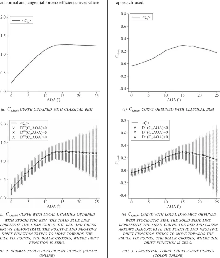
The results for normal and tangential force coefficients
are summarized in Figs. 2-3 respectively. The Fig. 2(a) and
Fig. 3(a) show the Cn,Static and Ct,Static curves as function of AOA obtained with classical BEM. The Fig. 2(b) and
Fig. 3(b) represent the Cn,Model and Ct,Model curves with local dynamics as function of AOA obtained with
stochastic BEM.
In Fig. 2(b) and Fig. 3(b), the drift function obtained with
Equation (4) presents the full map of local dynamics of the
normal and tangential force coefficients for each AOA.
Where, the red arrows display the deterministic increase
time and the green arrows display the deterministic
decrease of same parameters over the time. The black
crosses represent the stable fix points matching the usual
mean normal and tangential force coefficient curves where
drift function is zero. The curve consisting of stable fix
points (the black crosses) could be called Langevin normal
and tangential force coefficient curves based on the
approach used.
(a) Cn,StaticCURVE OBTAINED WITH CLASSICAL BEM
(b) Cn,ModelCURVE WITH LOCAL DYNAMICS OBTAINED
WITH STOCHASTIC BEM. THE SOLID BLUE LINE REPRESENTS THE MEAN CURVE. THE RED AND GREEN ARROWS DEMONSTRATE THE POSITIVE AND NEGATIVE
DRIFT FUNCTION TRYING TO MOVE TOWARDS THE STABLE FIX POINTS; THE BLACK CROSSES, WHERE DRIFT
FUNCTION IS ZERO.
FIG. 2. NORMAL FORCE COEFFICIENT CURVES (COLOR ONLINE)
(a) Ct,StaticCURVE OBTAINED WITH CLASSICAL BEM
(b) Ct,ModelCURVE WITH LOCAL DYNAMICS OBTAINED WITH STOCHASTIC BEM. THE SOLID BLUE LINE REPRESENTS THE MEAN CURVE. THE RED AND GREEN ARROWS DEMONSTRATE THE POSITIVE AND NEGATIVE
DRIFT FUNCTION TRYING TO MOVE TOWARDS THE STABLE FIX POINTS; THE BLACK CROSSES, WHERE THE
DRIFT FUNCTION IS ZERO.
Mehran University Research Journal of Engineering & Technology, Volume 33, No. 1, January, 2014 [ISSN 0254-7821]
The comparison of classical and stochastic BEM
approaches in terms of their contributed results in Figs.
2-3 demonstrate that the classical BEM based on static
tabulated airfoil data only provides the mean normal
and tangential forces. In comparison to this, the
stochastic BEM with integration of stochastic model
brings additional insight by expressing complete map
of the local force dynamics over the time. The mean
curves of the normal and tangential force local dynamics
show very good agreement with the mean curves
obtained with classical BEM. The Langevin force
coefficient curves shown in black crosses match almost
perfectly with the mean of the normal and tangential
force local dynamics.
5.
CONCLUSIONS
A stochastic lift and drag model has been integrated to
standard BEM model to achieve the dynamic forces on a
rotating blade element. The forces are obtained with local
dynamics for AOAs 0-25o at constant local radius and
constant pitch angle.
The comparison of classical and stochastic BEM
approaches demonstrate that the stochastic BEM brings
additional insight by expressing complete map of the
local force dynamics over the time. The classical BEM
based on static tabulated airfoil data only provides the
mean forces. The mean curves of the local force dynamics
show very good agreement with the mean curves
obtained with classical BEM. The Langevin force curves
shown in black crosses match almost perfectly with the
mean curves of the local force dynamics.
The model is being developed to extract and provide
the complete local loading information acting on the
wind turbine blades which could lead to an optimum
rotor design under turbulent wind circumstances. The
final goal is to achieve an aerodynamic model like
AeroDyn based on stochastic approach. Later it could
be combined with a wind energy converter model like
FAST or similar other model to obtain a stochastic rotor
model.
ACKNOWLEDGEMENTS
The authors would like to thank Joerge Schneemann for
access to his measured data. Also we would like to thank
the referees for their helpful comments and suggestions
for improvement of the paper.
REFERENCES
[1] Leishman, J.G., "Challenges in Modeling the Unsteady Aerodynamics of Wind Turbines", Wind Energy, Volume 5, Nos. 2-3, pp. 85-132, 2002.
[2] Morales, A., Waechter, M., and Peinke, J., "Characterization of Wind Turbulence by Higher Order Statistics", Wind Energy, Volume 15, No. 3, pp. 391-406, 2012.
[3] Boettcher, F., Barth, S., and Peinke, J., "Small and Large Scale Fluctuations in Atmospheric Wind Speeds", Stochastic Environmental Research and Risk Assessment, Volume 21, No. 3, pp. 299-308, 2007.
[4] Long, H., Wu, J., Mattew, F., and Tavner, P., "Fatigue Analysis of Wind Turbine Gear Box Bearings Using SCADA Data and Miner's Rule", Scientific Proceedings of EWEA, Brussels, Belgium, 2011.
[5] Muecke, T., Kleinhans, D., and Peinke, J., "Atmospheric Turbulence and its Influence on the Alternating Loads on Wind Turbines", Wind Energy, Volume 14, No. 2, pp. 301-316, 2011.
[7] Fuglsang, P., Antoniou, I., Dahl, K.S., and Madsen, H.A., "Wind Tunnel Tests of the FFA-W3-241, FFA-W3-301 and NACA 63-430 Airfoils", Scientific Report, Ris National Laboratory, No. Ris -R-1041(EN), Denmark, December, 1998.
[8] Fuglsang, P., Dahl, K.S., and Antoniou, I., "Wind Tunnel Tests of the Ris -A1-18, Ris -A1-21 and Ris -A1-24 Airfoils", Scientific Report, Ris National Laboratory, No. Ris -R-1112 (EN), Denmark, June, 1999. [9] Timmer, W.A., and Van Rooij, R.P.J.O.M., "Summary
of the Delft University Wind Turbine Dedicated Airfoils", Journal of Solar Energy Engineering, Volume 125, No. 4, pp. 488-496, 2003.
[10] Eggleston, D.M., and Stoddard, F.S., "Wind Turbine Engineering Design", Springer Publisher, 1st Edition, July 31, 1987.
[11] Leishman, J.G., "Principles of Helicopter Aerodynamics, Cambridge Aerospace Series", Cambridge University Press, 2nd Edition, April, 2006.
[12] Wolken-Moehlmann, G., Knebel, P., Barth, S., and Peinke, J., "Dynamic Lift Measurements on a FX79W151A Airfoil via Pressure Distribution on the Wind Tunnelwalls", Journal of Physics, Conference Series, Volume 75, No. 1, pp. 012026, 2007.
[13] Sant, T., "Improving BEM-Based Aerodynamic Models in Wind Turbine Design Codes", Phd Thesis, Delft University Wind Energy Research Institute, The Netherlands, 2007.
[14] Vermeera, L.J., Srensen, J.N., and Crespo, A., "Wind Turbine Wake Aerodynamics", Progress in Aerospace Sciences, Volume 39, Nos. 6-7, pp. 467-510, 2003. [15] Conlisk, A.T., "Modern Helicopter Rotor
Aerodynamics", Progress in Aerospace Sciences, Volume 37, No. 5, pp. 419-476, 2001.
[16] Snel, H., "Review of the Present Status of Rotor Aerodynamics", Wind Energy, Volume 1, No. S1, pp. 46-69, 1998.
[17] Ahlund, K., "Investigation of the NREL NASA/Ames Wind Turbine Aerodynamics Database", Scientific Report, Swedish Defence Research Agency, June, 2004.
[18] Hansen, M.O.L., and Madsen, H.A., "Review Paper on Wind Turbine Aerodynamics", Journal of Fluids Engineering, Volume 133, No. 11, pp. 114001, 2011. [19] Moriarty, P.J., and Hansen, A.C., "AeroDyn Theory
Manual", Technical Report, National Renewable Energy Laboratory, No. NREL/TP-500-36881, January, 2005. [20] Weinzierl, G., "A BEM Based Simulation-Tool for Wind Turbine Blades with Active Flow Control Elements", Diploma thesis, Technical University of Berlin, 2011. [21] Seoud, R.E., and Vassilicos, J.C., "Dissipation and Decay
of Fractal-Generated Turbulence", Physics of Fluids, Volume 19, No. 10, pp. 105108, 2007.
[22] Schneemann, J., Knebel, P., Milan, P., and Peinke, J., "Lift Measurements in Unsteady Flow Conditions", Scientific Proceedings of EWEC, Warsaw, Poland, 2010. [23] Risken, H., "The Fokker-Planck Equation", Springer
Publisher, 2nd Edition, 1996.
[24] Siegert, S., Friedrich, R., and Peinke, J., "Analysis of Data Sets of Stochastic Systems", Physics Letters-A, Volume 243, Nos. 5-6, pp. 275-280, July, 1998. [25] Kolmogorov, A.N., "Ueber Die Analytischen Methoden
in Derwahrscheinlichkeitsrechnung", Mathematische Annalen, Volume 104, No. 1, pp. 415-458, 1931. [26] Gottschall, J., and Peinke, J., "On the Definition and
Handling of Different Drift and Diffusion Estimates", New Journal of Physics, Volume 10, No. 8, pp. 083034, 2008.
Mehran University Research Journal of Engineering & Technology, Volume 33, No. 1, January, 2014 [ISSN 0254-7821]
[28] Press, W.H., Teukolsky, S.A., Vetterling, W.T., and Flannery, B.P., "Numerical Recipes in C The Art of Scientific Computing", Cambridge University Press, 2nd Edition, 1992.
[29] Luhur, M.R., Waechter, M., and Peinke, J., "Stochastic Modeling of Lift and Drag Dynamics under Turbulent Conditions", Scientific Proceedings of EWEA, Copenhagen, Denmark, 2012.
[30] Burton, T., Sharpe, D., Jenkins, N., and Bossanyi, E., "Wind Energy Handbook", John Wiley & Sons, UK, 2002.
[31] Buhl, M.L.Jr., "A New Empirical Relationship between Thrust Coefficient and Induction Factor for the Turbulent Windmill State", Technical Report, National Renewable Energy Laboratory, No. NREL/TP-500-36834, August, 2005.
[32] Glauert, H., "A General Theory of the Autogyro", ARCR R&M No. 1111, 1926.