New Concept of PLC Modems: Multi-Carrier System for Frequency Selective Slow-Fading Channels Based on Layered SCCC Turbocodes

New Concept of PLC Modems:

Multi-Carrier System for Frequency Selective

Slow-Fading Channels Based on Layered SCCC

Turbocodes

Jan ZAVRT ´

ALEK, Daniel KEKRT, Jarom´ır HRAD

Dept. of Telecomm. Engineering, Czech Technical University in Prague, Technick´a 2, 166 27 Praha, Czech Republic

zavrtjan, kekrtd1, [email protected]

Abstract. The article introduces a novel concept of a PLC modem as a complement to the existing G3 and PRIME stan-dards for communications using medium- or high-voltage overhead or cable lines. The proposed concept is based on the fact that the levels of impulse noise and frequency se-lectivity are lower on high-voltage lines than on low-voltage ones. Also, the demands for “cost-effective” circuitry design are not so crucial as in the case of modems for low-voltage level. In contract to these positive conditions, however, there is the need to overcome much longer distances and to take into account low SNR on the receiving side. With respect to the listed reasons, our concept makes use of MCM, instead of OFDM. The assumption of low SNR is compensated through the use of an efficient channel coding based on a serially concatenated turbo code. In addition, MCM offers lower latency and PAPR compared to OFDM. Therefore, when us-ing MCM, it is possible to excite the line with higher power. The proposed concept has been verified during experimental transmission of testing data over a real, 5 km long, 22 kV overhead line.

Keywords

Power line communication, multi-carrier modulation, serially concatenated convolutional codes, iterative detection, BCJR forward-backward algorithm, soft-output Viterbi algorithm, soft-in soft-out module, expectation-maximization algorithm, soft decision di-rected synchronization, data aided synchronization, joint iterative synchronization and detection

1. Introduction

Reliable and fast power line communication (PLC) is a key prerequisite for successful deployment and operation of Smart Grid networks. At present, only the communication over low-voltage power lines is largely used, thanks to rel-atively inexpensive hardware, mainly for Automatic Meter Reading (AMR), tariffs and load management (Automatic Meter Management, AMM), and complex monitoring of

network infrastructure (Advanced Metering Infrastructure, AMI) in order to increase the reliability of power distribu-tion, which is the last step on the way towards a Smart Grid. Networks are usually controlled from substations and dis-tribution stations, using (1) medium- or high-voltage power line, (2) dedicated data link (Internet, dedicated data circuit, optical cable, etc.). It is only logical to use the existing medium-voltage power lines for data communication, thus eliminating the need of a dedicated data link. Such solution can reduce the dependence on external factors and thereby increase the reliability of power distribution networks. Due to rapid deployment of so-called renewable energy sources, the reliability and stability of the network is becoming a se-rious problem.

LTS LFTS

LPTS TS

g(t) =G(fmin+ 2.5B, t)

B(MCM) _fmax

fmin B G(f, t)

Frame

FSP

time

freq.

P

ack

et

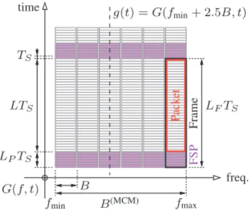
Fig. 1.Time-frequency partition of packets for serial MCM.

In this article we propose a novel communication sys-tem, designed specifically for communication over medium-voltage (mv) power lines. Its purpose is to fill the gap in the existing systems based on OFDM (like G.hnem, IEEE P1901.2, G3, PRIME), since their robustness is somewhat lower when they are used for long-distance transmission over medium-voltage power lines.

The architecture of the proposed solution is based on the assumed physical characteristics of the transmission me-dia (i.e. medium-voltage overhead or cable lines) that feature moderate frequency selectivity within CENELEC A band and high levels of noise. The type of the noise, in gen-eral, is AWGN (Additive White Gaussian Noise). In such

samplingnTp

samplingℓTs

˜

s(MCM)_(t) nTp

˜

sK

[

n

]

˜

s2

[

n

]˜

s1

[

n

]

˜

s

(MCM)

[

n

]

d₁[ℓ]

d₂[ℓ]

d

K[ℓ]

ejω₁nTp

ejω2nTp

ejω_KnTp

d(S)

1 [ℓ

′_]

q1[ℓ] q1[ℓ]

d(S)

2 [ℓ

′_]

d(S) K[ℓ

′_] q2[ℓ]

qK[ℓ]

q2[ℓ]

qK[ℓ]

s2[n]

sK[n]

s1[n]

Carry wave 2

ℜ(.)

generator

wave KCarry

generator

wave 1Carry

ℜ_(.)

ℜ_(.)

generatorclock

Transmitter

DAC

Analog interpolator

LPF generator

insertion (service data)

FSP

(service data) Turbocode

SCCC Layered

FSP

TurbocodeSCCC Layered

modulator Layered

SCCC Turbocode

digital modulator

digital Linear

Linear FSP

(service data) insertion

modulator digital Linear

insertion

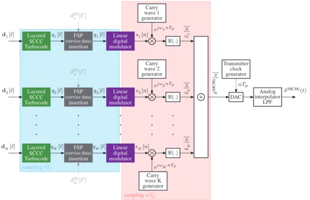
Fig. 2.Block diagram of a transmitter for serial MCM.

case, the OFDM (Orthogonal Frequency Division Multiplex-ing) technology is not suitable because of its high PAPR (Peak-to-Average Power Ratio) - it should be used rather for channels with high frequency selectivity, or significant multipath signal propagation. Moreover, OFDM introduces high processing latency in the receiving digital front-end, as it uses FFT and IFFT integral transforms. The latency can be partially reduced by shortening of the OFDM frame; however, it results in lower spectral efficiency (number of

carriers). Another technology to be considered is

wide-band single-carrier linear digital modulation, which has low PAPR, but it is not immune against frequency selectivity. In a frequency-selective channel, it requires equalization at the receiving side, computationally intensive channel estimation and a complicated core for channel inversion. For these rea-sons we propose MCM (Multi-Carrier Modulation) as the optimum technology for data communication over mv power lines, i.e., a set of subchannels using narrowband linear digital modulations, with equidistantly or non-equidistantly spaced carriers over the given bandwidth. Such approach offers sufficiently low PAPR, and also very low processing latency (only matched filtering is performed on the receiving side). Every subchannel is considered as frequency-flat, and therefore no equalization is needed - only simple synchro-nization of amplitude, phase and symbol timing is required.

The paper is organized as follows. Section 2 describes Serial MCM transmission. Sections 3 and 4 describes MCM Transmitter and Receiver. Section 5 describes experimental measurement. Finally, Section 6 presents conclusions and ideas for future work.

2. Serial MCM Transmission

The proposed architecture of MCM PLC modem is based on serial data transmission. The individual subchan-nels are entirely independent, carrying separate data commu-nications at lower bitrate, corresponding to the subchannel bandwidth. If SNR in some of the subchannels is negatively affected by strong noise, interference or destructive defor-mation (gap) in channel frequency response, the data is di-rected to other subchannels where the conditions are better. So, the concept is based on the assumption that transmission conditions are not bad across the entire MCM band.

The individual data packets are split into subchannels in time-frequency domain as described in Fig. 1, and their transmission may but need not be entirely independent. FSP (Frame Synchronization Preamble) stands for synchroniza-tion preamble of a frame containingLPchannel symbols,TS

is symbol period,L andLF mean packet length and frame

length, respectively, expressed as the number of channel

symbol,BandB(MCM)mean subchannel bandwidth and

to-tal modulation bandwidth, respectively, andG(f,t)is time-frequency transfer function of the channel.

3. Transmitter Description

q[ℓ] Pulse shaping (SqRRCS)

s[n′_] qp[n′]

Linear digital modulator

Zero padding

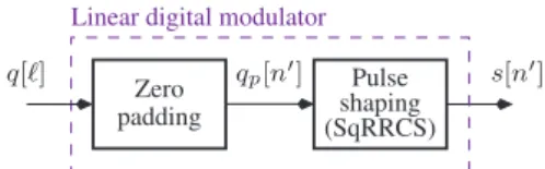
Fig. 3.Block diagram of a linear digital modulator.

3.1 Transmitter Digital Front-End

Every branch of the structure represents one subchan-nel of the resulting composite spectrum. Each particular section of the resulting spectrum is shaped in a narrowband linear digital modulator through a complex filter with real SqRRCS (Square Root Raised Cosine Spectrum) impulse re-sponse, as shown in Fig. 3.

3.2 Turbo Encoders

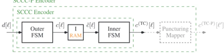
Noise immunity is achieved through channel coding based on punctured serial concatenated turbo code, see Fig. 4. At present, it is one of the most efficient channel coding techniques. Its coding gain grows with the length of the encoded packet. This is the only negative property of turbo coding, as it implies limitation for transmission of short packets; suitable packet lengths are 1024 or more sym-bols. More information about turbo codes can be found in [1]-[4].

For the proposed concept we have chosen a proven ar-chitecture, in which the outer FSM (Finite State Machine) is based on a simple systematic forward- or backward-recursive convolution code. The FSM has 2 or 4 internal states. The fixed code rate is 1/2, i.e. the coder adds one protective (redundant) bit to each bit of the information. So, there is a binary data sequenced[]at the input of the coder, and another sequencec[]at its output, in modulo 4

arith-metic. The sequence c[]is taken to the permutator I and

then passed to the inner FSM. The inner FSM is based on a simple integrator with 4 internal states and 1/1 rate. The fixed turbo code rate is 1/2, and the code symbolsc(TC)[]at the output can be directly mapped to the QPSK constellation, with respect to Ungerboeck mapping rules.

If the transmission conditions are good and SNR (Signal-to-Noise Ratio) high, then the modem switches to layered turbo code mode (see Fig. 5), in which the data are transmitted in 2, 3 or 4 streams hierarchically mapped to

16QAM, 64QAM or 256QAM, andKequals to 4. Thanks

to the hierarchical mapping, the individual data streams have different priorities: stream #1 has the highest priority, while stream #4 the lowest one. The reason is that stream #1 is mapped to the highest-quality points of QAM constella-tion (i.e. those with the largest mutual Euclidean distances). Therefore the noise immunity of stream #1 will be very high, at the expense of stream #4 that is mapped to the lowest-quality points, thus having low noise immunity. If all data streams are required to behave equally, a commutator is prepended to the mapper input; then hierarchical mapping

will be rotated over the time, and so the respective noise im-munities of the individual streams will be equalized. Besides the hierarchical mapping, the proposed concept allows also modification of the initial code rate using the punctured map-ping. Suitable puncturing changes the initial code rate 1/2 to the output code rates 2/3 and 3/4. When the SNR is low, the transmitter uses the default code rate 1/2. As the SNR grows, the transmitter is switched firstly to the rate 2/3, and subse-quently to 3/4. Code rates of all considered modem con-figurations along with the assumed SNR requirements are summarized in Tab. 1. The overview refers to MCM with total bandwidth of 80 kHz consisting of 8 subbands, 9.5 kHz each, separated by 0.5 kHz gaps; the centers of the individual channels are at 40 kHz, 50 kHz, 60 kHz, ..., 110 kHz.

4. Receiver Description

Block diagram of the receiving side is shown in Fig. 6. The receiver consists of three fundamental blocks: digital front-end, multilayer frame synchronization block, and a set of joint iterative synchronizers-detectors allocated through a switch.

4.1 Receiver Digital Front-End

The individual subchannels are firstly mixed with the corresponding subcarriers to obtain a set of signals (complex envelopes) in baseband. Then these baseband signals are decimated in a down-sampling cascade consisting of a se-ries of anti-aliasing filters and decimators (CIC filter). At its output we get sub-sampled complex envelopesrk[n′]so

that there are 4 samples per or one symbol period, which is perfectly in accord with the sampling theorem. The par-ticular sub-sampled complex envelopes are then shaped and partially rid of AWGN in matched filters with real impulse response SqRRCS. Consolidated complex envelopes at the output of the matched filtersxk[n′]are then passed to a set of

frame synchronizers.

4.2 Frame Synchronization

Frame synchronizers search for synchronization

preambles in the individual streams, which are used to local-ize the beginnings of particular packets (frame synchroniza-tion), and also for initial estimates of subchannel attenuation |gˆ(_k0)|, phase rotation _gˆ(0)

k , symbol timing ˆτ (0)

k and standard

deviation of AWGN ˆσ(_w0)

k. These values are estimated

us-ing Data Aided (DA) Maximum-Likelihood (ML) Channel State Estimators (CSE), which are autonomous functional sub-blocks of the frame synchronizers.

c[ℓ]

d[ℓ] ˜c[ℓ] _c(TC)_[ℓ] c(TC-P)_[ℓ′_]

Inner FSM FSM

Outer I

RAM

SCCC Encoder

Puncturing Mapper

SCCC-P Encoder

Fig. 4.Block diagram of a punctured serial turbo coder.

q_k[ℓ] d_k,1[ℓ]

d

k[ℓ]

dk,2[ℓ]

d_k,K′[ℓ]

c(TC)k,1 [ℓ]

c(TC)k,K′[ℓ] c(TC)k,2 [ℓ]

Hierarchical

QAM

Mapper

Commutator

Layered SCCC Turbocode

SCCC Turbocode

Turbocode Turbocode SCCC

SCCC

Fig. 5.Block diagram of a layered serial turbo coder.

prefix, the lengths can be extended to even bits count suit-able for practical implementation. The second option is to use a pair of R-S preambles, which can be used to trans-mit a very slow, but very robust binary stream called service data. The principle of transmitting service data is quite sim-ple. Let us select one R-S preamble from the pair, according to the value of the input bitd_k(S)[′]. On the receiving side, so-called dual version of frame synchronizer is then used, which searches for both of the R-S preambles. Its output is

ˆ

d_k(S)[′_{]estimate depending on the detected R-S preamble.}

The bitrate of service data depends on the length of a packet and of the used R-S preambles including the cyclic prefix – see Tab. 1. The default lengths of these training sequence pairs are 2l, wherel=1,2,3, ...,N.

4.3 Joint Iterative Synchronizer-Decoder

Samples of complex envelope, isolated by frame syn-chronizers and corresponding to one data packet in each sub-channel, are passed through the switch to the joint iterative synchronizer-detector – see Fig. 7. Together with this sec-tion, the initial estimates of ˆg(_k0), ˆτ(0)

k and ˆσ

(0)

wk are handed

over. Processing of the complex envelope begins in so-called Soft Output Demodulator (SODEM) shown in Fig. 8. Firstly, the complete envelope section is stored into RAM memory of the demodulator. Then it is resampled and decimated in Decimator-Interpolator (DFA) based on Farrow algorithm. The resampling is controlled by symbol timing estimate ˆτ(I)_. At the DFA output we get time-synchronized sequence of

channel symbolsxh[]. These symbols are then corrected in

amplitude and phase, depending on channel estimate ˆg(I)in order to obtain fully synchronized sequence of channel sym-bolsxh[]. The differences between received channel

sym-bolsxh[]and transmitted symbolsq[]are then caused only

by superimposed AWGN noise; now the logarithmic likeli-hood function or forward detector metrics{

M

F }(discrete

probability density) can be computed, with respect to the es-timate of AWGN standard deviation ˆσ(I)_{w .}

The forward metrics of

M

F (qˇk) proceed into

di-vider/combiner logic of so-called soft inversion of Hierar-chic QAM Mapper, the output of which provides compos-ite (layered) forward metrics ˆ

M

F (cˇ

(TC)

k,k′ ). These metrics are used as an input for the individual Iterative Decoding Networks (IDN) of the Serially Concatenated Convolutional Codes (SCCC) – see Fig. 9. The arrangement of the decod-ing network is equivalent to the structure of turbo coder. So, if punctured turbo code is used on the transmitting side, then the corresponding IDN at the input is prepended by soft in-version of the puncturing mapping block SOM (Soft-Output Mapper). The fundamental components of SCCC IDN are Soft-In Soft-Out (SISO) soft inversion blocks of convolution coders FSM on the transmitting side. The SISO modules perform Forward-Backward Algorithm (FBA), also known as BCJR (Bahl, Cocke, Jelinek and Raviv). More informa-tion about BCJR algorithm and its derivatives can be found in [1]-[3] and [5]-[8]. A two-dimensional BCJR algorithm can be found in [12].

The outputs of the particular detection layers are packet data estimates ˆdk,k′[] and partial (layer) backward metrics

ˆ

M

B (cˇ

(TC)

k,k′ ). The hard data estimate ˆdk,k′[]is computed in the Decision block (DEC) by thresholding of output forward metrics ˆ

M

F (dˇk). The backward partial metrics ˆ

M

B (cˇ

(TC)

k,k′ )

are then combined into backward metrics ˆ

M

B (qˇk)that are

immediately transformed, together with the forward metrics ˆ

M

F (qˇk), into posterior probabilities ˆ

P

se-quence of ˆ

P

im-proves the initial estimates of ˆg(_k0), ˆτ(0)

k and ˆσ (0)

wk.

In this concept it is based on the Expectation-Maximization (EM) criterion, Soft Decision Directed (SDD) by ˆ

P

samplingn′_T′ p samplingnTp

samplingℓTs

ˆ d₁[ℓ]

ˆ d_2[ℓ]

ˆ d

K[ℓ]

2e−jω

KnTp τˆ

(0) K

ˆ

g(0)K

ˆ

g(0)1

ˆ

τ1(0)

ˆ

g(0)2

ˆ

τ2(0)

Switch control ˆ

σw(0)_K xK[n′]

2e−jω₁nTp

2e−jω₂nTp

˜ r (MCM) [ n ]

x1[n′]

ˆ

σw(0)₁

Switch control

Switch control

ˆ

σw(0)2

x2[n′]

ˆ

d(S) K[ℓ

′_] ˆ

d(S)

2 [ℓ

′_] ˆ

d(S)

1 [ℓ

′_]

˜

r(MCM)_(t) nTp

Matched filter generatorclock Receiver (SqRRCS) (SqRRCS)filter Matched ADC

Sync & Det. (branch 1)

Switch rK[n′]

r2[n′]

Joint iter.

(Dual) frame sync

(branchKb)

Sync & Det.Joint iter.

(Dual) frame sync

Joint iter. Sync & Det.

(branch 2) (Dual) frame sync

Matched filter (SqRRCS) Carry wave 1 generator Carry wave K generator

generatorwave 2

Carry

Switch r1[n′]

logic Sw. control ML CSE Data aided logic Sw. control logic Sw. control ML CSE Data aided Data aided ML CSE sampling Down-cascade cascade Down-sampling sampling Down-cascade

Fig. 6.Block diagram of a receiver using serial MCM.

ˆ

dk,2[ℓ]

ˆ

d_k,K′[ℓ] ˆ

dk,1[ℓ]

ˆ P(I)_(ˇqk)

ˆ d

k[ℓ]

ˆ τ ( I ) k _ˆ g ( I ) k ˆ M(_FI)( ˇdk,1)

ˆ σ ( I ) w k ˆ M(_FI)(ˇc(TC)k,1)

ˆ

σw(0)k

ˆ

τk(0)

ˆ

g(0)k

ˆ

τ

(

I

+1)

k (I _ˆg

+1)

k

ˆ M(I)

F ( ˇdk,K′)

ˆ σ ( I +1) wk ˆ M(I)

B ( ˇdk,2)

ˆ M(I)

F (ˇc (TC) k,K′)

x

k[ℓ]

ˆ M(_BI)_{( ˇd}

k,K′) ˆ

M(I)

B (ˇqk)

ˆ M(_BI)_(ˇc(TC)

k,K′)

ˆ M(I)

B ( ˇdk,1)

ˆ M(I)

B (ˇc (TC) k,2)

ˆ M(_FI)(ˇqk)

ˆ

M(_FI)(ˇc(TC)k,2) Mˆ

(I) F ( ˇdk,2)

ˆ M(I)

B (ˇc (TC) k,1)

RAM DEC FWMs RAM DEC RAM FWMs RAM BWMs Joint iterative synchronizer-detector

DEC Commutator Hierarchical QAM Soft-output Mapper &

exp(.)

Combiner BWMs RAM BWMs RAM RAM SODEM & Switch RAM Joint SS SDD EM CSE FWMs RAMs IDN SCCC RAMs Md-SqD IDN SCCC IDN Md-SqD SCCC Md-SqD RAMs J I

Fig. 7.Block diagram of the layered synchronizer-detector.

for synchronization acquisition mode and for receiver track-ing mode. Detailed description of the EM algorithm provid-ing basic synchronization of the iterative decodprovid-ing network can be found in [17] and [20]. More variants of EM and its derivatives are discussed in [14]-[16] and [18]. Another approach to decoding network synchronization based on so-called adaptive SISO modules, can be found in [19].

The updated estimates of ˆg(I)_k , ˆτ(I)

k and ˆσ (I)

wk are

redi-rected into the Soft Demodulator, and so one iterationI of

the system is completed. In the next iteration the whole de-tection process is repeated with the updated estimates. After performing the given maximum number of iterations or after stabilization of the iterative network, the estimateˆdk[]at the

System Packet Preamble Subchannel Modulation User data Service data

variant length length Alphabet bitrate bitrate bitrate bitrate Usage [bits] [bits] [kbit/s] [kbit/s] [kbit/s] [bit/s]

1024 40 QPSK 8.44, 67.55, 65.01,86.68,97.52 63.50

Turbocode 2048 40 QPSK 11.25, 90.06, 66.26,88.34,99.39 32.40 Very low

4096 40 QPSK 12.66 101.32 66.90,89.20,100.35 16.30 SNR>4 dB

rate 1/2,2/3,3/4 8192 40 QPSK 67.22,89.62,100.83 8.20 Double-layer 1024 40 16QAM 16.90, 135.11, 130.03,173.37,195.04 63.50

turbocode 2048 40 16QAM 22.53, 180.14, 132.52,176.69,198.78 32.40 Low 4096 40 16QAM 25.35 202.67 133.80,178.40,200.70 16.30 SNR>10 dB rate 1/2,2/3,3/4 8192 40 16QAM 134.45,179.27,201.68 8.20

Triple-layer 1024 24 64QAM 25.30, 202.66, 198.02,264.02,297.03 64.50

turbocode 2048 24 64QAM 33.73, 270.21, 200.32,267.08,300.47 32.60 Medium 4096 24 64QAM 37.95 303.99 201.48,268.64,302.22 16.40 SNR>16 dB rate 1/2,2/3,3/4 8192 24 64QAM 202.07,269.42,303.11 8.22

Quadruple-layer 1024 24 256QAM 33.80, 270.22, 264.03,352.03,396.04 64.50

turbocode 2048 24 256QAM 45.07, 360.28, 267.09,356.11,400.63 32.60 High 4096 24 256QAM 50.70 405.33 268.64,358.18,402.97 16.40 SNR>22 dB rate 1/2,2/3,3/4 8192 24 256QAM 269.43,359.23,404.14 8.22

Tab. 1.Modem configuration summary.

it is passed for further processing by the higher layers of the modem.

5. Experimental Measurement

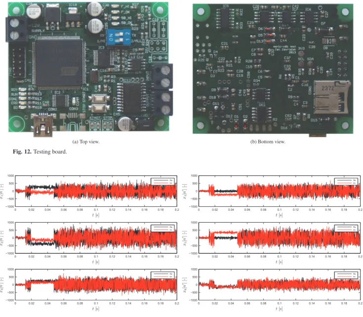
The transmitter consists of an SD-card memory, a con-troller, 16-bit DA converter and a wideband Tx amplifier. A signal generated from MATLAB was stored in the SD-card memory. The signal contained 3600 different pack-ets with random data. It was periodically transmitted into the power line at voltage level of 1 Vrms. The Tx

am-plifier output impedance wasZS=68Ω resistive. The

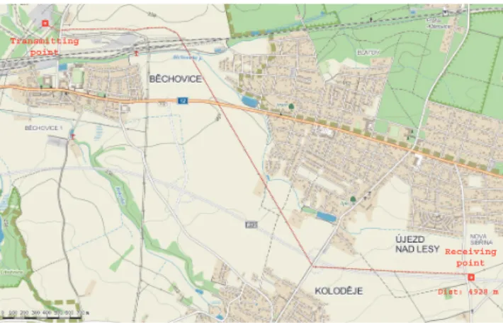
re-ceived signal went through a 1st-order RC high-pass filter with cut-off frequency of 1.5 kHz to remove the 50 Hz com-ponents. Then it was received using a storage oscilloscope Tektronix DPO4032. The received signal was processed of-fline in MATLAB. The power line was a 4928 m long three-phase 22 kV overhead line (system with non-grounded neu-tral point); it is shown in Fig. 10. The line runs from a substa-tion approximately 700 m in parallel with three other 22 kV power lines and a 3 kV DC railway trolley. Then it crosses the railway and runs separately (see Fig. 10). The power line direction is towards a nearby MW radio transmitter at

620 kHz, which induced 1.1 Vrms signal into a 68Ω_load

connected between L1 and GND. Two measurement setups were used (see Fig. 11). In the first setup, (Fig. 11b), the measuring signal was injected between phase L1 and GND. GND was connected to the substation’s common ground-ing point; this means that considerable 50 Hz current from other transformers’ neutrals in the substation went through GND. Another anticipated source of GND noise was the railway trolley [23]. On the receiving side in the field, it was grounded using the grounding strip of the disconnector

(equipment of the pole). In the second setup (Fig. 11a), the signal was injected between phases L1 and L2. In this setup, the noise level was substantially lower. More information about the line, coupling unit and measurement that helped to design the measurement can be found in [24]-[28].

ˆ M(I)

F (ˇq) x[n]

x_[ℓ]

xh[ℓ]

ˆ

τ(I) _ˆg(I) _ˆσ(I) w

RAM

metrics Forward

RAM

observation Rx

Decimation DFA interpolator

Log. likelihood

function

SODEM

Fig. 8.Block diagram of the soft-output demodulator.

5.1 Testing Board Description

sig-ˆ M(I)

B (ˇc(TC))

ˆ M(I)

F (ˇc(TC)) Mˆ

(I) F ( ˇd)

ˆ M(I)

B ( ˇd)

ˆ M(I)

F (ˇc) ˆ

M(I)

F (ˇc(TC-P))

ˆ M(I)

B (ˇc(TC-P)) Mˆ

(I) B (ˇc)

ˆ M(I)

B (ˇ˜c)

ˆ M(I)

F (ˇ˜c)

RAM

I

RAM

I−1 _Outer

RAM

States

SISO

FI FBA

RAM serial

Md-SqD Md-SqD

FI FBA SISO Inner

SCCC IDN

Puncturing SOM

schedule activation

States

SCCC-P IDN

I

Fig. 9.Block diagram of the iterative detection network.

nal onto SD card memory. First channel is unfiltered (raw) signal from power line, second channel is the same signal filtered by high pass filter to obtain higher dynamic range in frequency band of interest. The amplitude level indicator helps to set input voltage divider to avoid signal clipping and saturation of ADC. For the purposes of analyses in this arti-cle, only TX mode was used because of low ADC sampling frequency.

5.2 Developed Modem Performance Analysis

Performance analysis of the proposed concept was based on periodic transmission of a testing sequence (modu-lated signal) into a 22 kV power line from a substation, and subsequent detection of the received signal using a digital storage oscilloscope – see Fig. 10. The modulated MCM sig-nal used 6 subchannels, each of them containing 600 packets composed of 256 symbols. So, 3600 different packets were analyzed during one run. The subchannels (carriers) were centered at frequencies from 30 kHz to 80 kHz with 10 kHz step, and the total MCM signal bandwidth was 84.75 kHz. In every subchannel we used linear QPSK modulation with SqRRCS modulation impulse with relative length of 12 sym-bol periods and rolloff factor of 0.0667. Usable subchan-nel bandwidth was 9.5 kHz and symbol rate was 8.906 kBd. The DAC sampling frequency of 187.5 kHz creates Nyquist zone 93.75 kHz wide, into which the entire MCM modu-lation could fit with sufficient margin. With respect to the sampling frequency and other parameters listed above, the resulting symbol period was 0.1123 ms, and one symbol pe-riod corresponds to 20 samples of the modulated signal.

Serial single-layer (K′=1) turbo code with code rate of 1/2 without puncturing (see Fig. 4) was used as channel coder. Subchannel bitrate was 8.906 kbit/s, so MCM total bitrate was 53.4366 kbit/s. A redundant systematic back-ward recursive convolution coder having 4 internal states, 8 trellis transitions and code rate of 1/2 was used outer coder. A discrete integrator with a code rate of 1/1 and modulo 4 arithmetic was used as inner coder.

point point

Transmitting

Receiving

Dist: 4928 m

Fig. 10.Power line used for the experimental transmission.

L1

L2

L3

ZS ZL

Rx powerline

Tx L3

L2

L1 ZL

GN D

ZS

Tx

powerline

Rx

(a) Transmission between two

phases.

(b) Transmission between a phase and ground.

/

L1 L2 L3 1.75 m 1.75 m

12 m

(c) Dimensions of a electric pole of the measured power line.

(a) Top view. (b) Bottom view.

Fig. 12.Testing board.

0 0.02 0.04 0.06 0.08 0.1 0.12 0.14 0.16 0.18 0.2

−1000 −500 0 500 1000

t[s]

x1

[

n

′][

-]

Re Im

0 0.02 0.04 0.06 0.08 0.1 0.12 0.14 0.16 0.18 0.2

−1000 −500 0 500 1000

t[s]

x2

[

n

′][

-]

Re Im

0 0.02 0.04 0.06 0.08 0.1 0.12 0.14 0.16 0.18 0.2

−1000 −500 0 500 1000

t[s]

x3

[

n

′][

-]

Re Im

0 0.02 0.04 0.06 0.08 0.1 0.12 0.14 0.16 0.18 0.2

−1000 −500 0 500 1000

t[s]

x4

[

n

′][

-]

Re Im

0 0.02 0.04 0.06 0.08 0.1 0.12 0.14 0.16 0.18 0.2

−1000 −500 0 500 1000

t[s]

x5

[

n

′][

-]

Re Im

0 0.02 0.04 0.06 0.08 0.1 0.12 0.14 0.16 0.18 0.2

−1000 −500 0 500 1000

t[s]

x6

[

n

′][

-]

Re Im

Fig. 13.Complex envelopes of the first 5 received packets.

Serial approach was applied to the packet transmission – see Fig. 1. After subtracting the synchronization overhead (Rudin-Shapiro preambles), the resulting bitrate available for user data is 46.2154 kbit/s. The MCM signal was trans-mitted repeatedly with idle periods between the repetitions. The beginning of MCM signal in all subchannels was indi-cated by an empty (null) packet, which helps to easily find the beginning of the received sequence and to extract the seg-ment of the received signal. The complete extracted segseg-ment was subsequently analyzed in MATLAB, including determi-nation of error rate through comparing of the received se-quence with reference data. The same segment of the testing MCM signal was used for transmission between two phases (Fig. 11a) and between a phase and ground (Fig. 11b). The received signal was always sampled at 250 kHz; so, resam-pling to 187.5 kHz was needed before further processing of the received signal, using a digital interpolator based on Far-row algorithm.

Figure 13 shows complex envelopes of the first 5 pack-ets of the testing sequence at the output of the matched filter,

using the measurement setup from Fig. 11a. The number of samples per symbol period of the envelope on the receiv-ing side was set to 4. Graphs in Fig. 13 clearly show the empty (null) leading packets preceded by the synchroniza-tion Rudin-Shapiro preambles containing 32 symbols, ex-tended with 8 symbols of cyclic prefix to the total length of 40 symbols. Every packet begins with one of the two Rudin-Shapiro preambles, depending on the service data stream with average bitrate of 0.1805 kbit/s for the entire MCM bandwidth.

The same complex envelopes are shown also in Fig. 14; Figure 14a shows their spectra, and Fig. 14b constellations. The empty (null) packets are again clearly visible as dense clusters of samples.

−20 −10 0 10 20 10 −10 10 −8 10 −6 10 −4 10 −2 10 0 f[kHz] X1 ( f )

−20 −10 0 10 20

10 −10 10 −8 10 −6 10 −4 10 −2 10 0 f[kHz] X2 ( f )

−20 −10 0 10 20

10 −10 10 −8 10 −6 10 −4 10 −2 10 0 f[kHz] X3 ( f )

−20 −10 0 10 20

10 −10 10 −8 10 −6 10 −4 10 −2 10 0 f[kHz] X4 ( f )

−1000 −500 0 500 1000

−1000 −500 0 500 1000

ℜ(x1[n′]) [-]

ℑ ( x1 [ n ′]) [-]

−1000 −500 0 500 1000

−1000 −500 0 500 1000

ℜ(x2[n′]) [-]

ℑ ( x2 [ n ′]) [-]

−1000 −500 0 500 1000

−1000 −500 0 500 1000

ℜ(x3[n′]) [-]

ℑ ( x3 [ n ′]) [-]

−1000 −500 0 500 1000

−1000 −500 0 500 1000

ℜ(x4[n′]) [-]

ℑ ( x4 [ n ′]) [-]

−20 −10 0 10 20

10 −10 10 −8 10 −6 10 −4 10 −2 10 0 f[kHz] X5 ( f )

−20 −10 0 10 20

10 −10 10 −8 10 −6 10 −4 10 −2 10 0 f[kHz] X6 ( f )

−1000 −500 0 500 1000

−1000 −500 0 500 1000

ℜ(x5[n′]) [-]

ℑ ( x5 [ n ′]) [-]

−1000 −500 0 500 1000

−1000 −500 0 500 1000

ℜ(x6[n′]) [-]

ℑ ( x6 [ n ′]) [-]

(a) Spectra. (b) Constellations.

Fig. 14.Spectra and constellations of the first 5 received packets.

or 2nd Rudin-Shapiro preamble. At the output of the internal CSEs there are three basic estimates: initial subchannel sym-bol timing LAG est.≡τˆ(0)_{, initial subchannel transfer} func-tion CSI est.≡gˆ(0), and initial subchannel signal-to-noise ratio SNR est.∝σ_ˆ(_w0)_{(not shown in Fig. 15).}

The outputs of the internal CSEs are immediately used in frame synchronizers to compute logarithmic likelihood functions corresponding to the 1st and 2nd Rudin-Shapiro preamble; Figure 16 shows the values of these functions for the first 5 received packets. The difference between these likelihood functions provides the resulting statistic (LLFR). LLFR is then compared to the threshold given by reduced

en-ergy of subchannel complex envelope (±THR.). If LLFR

ex-ceeds the value of THR, the beginning of a packet is detected along with the corresponding bit of service data stream.

Now let us leave the zoomed area of the first 5 packets transmitted between two phases, as illustrated in Fig. 11b, and have a look on time lapse graphs of the whole transmis-sion to compare both arrangements. Figure 17 shows the key control statistics of the receiver. First of all, every transmit-ted packet contains its 7-bit identification number (ID) that is used for packet loss analysis. Peak triplet flag indicates time spacing of synchronization peaks at the output of frame synchronizer; this flag shows whether both synchronization peaks of the previous and of the next packet occur in correct time interval - therefore the evaluation of the Peak triplet flag is delayed by one packet. If the synchronization peaks can-not be localized, the flag is set to zero, which means (false)

frame synchronization alarm or another error on the receiv-ing side. These two statistics together influence the value of packet Validity flag; a packet is considered to be valid if the extracted ID fits into the assumed sawtooth sequence and the Peak triplet flag is not set to zero.

Figure 18 shows symbol error rates (SER) of the re-ceived packets. It is visible that the transmission between a phase and ground (Fig. 18b) suffered from higher noise levels, and therefore the symbol error ratio is higher than for transmission between two phases (Fig. 18a). In both cases we can see decreased SER after repeated iterations of SO-DEM in Fig. 7. The most attenuated and most noisy sub-channel in both cases was the subsub-channel number 6. All the other channels were decoded with almost no errors during the whole transmission. Rarely there appear packets with very high symbol error rate, which almost leads to their loss; these situations cause singular faults of symbol timing syn-chronization in receiver tracking mode, i.e. inside the SO-DEM loop in Fig. 7. The speed of convergence towards cor-rect data estimates during SODEM iterations depends also on packet length. In this experiment we used relatively short packets of 256 symbols, due to time constraint. For prac-tical use it is necessary to transmit packets with minimum length of 1024 symbols in order to increase the turbo code performance.

in-0 1000 2000 3000 4000 5000 6000 7000 0

0.5 1

n′_[-]

LA

G

es

t.

[-] CH 1 CH 2 CH 3 CH 1 CH 2 CH 3

0 1000 2000 3000 4000 5000 6000 7000

0 2 4 6 8 10

n′_[-]

| CS I | es t.

[-] CH 1 CH 2 CH 3 CH 1 CH 2 CH 3

0 1000 2000 3000 4000 5000 6000 7000

−4 −2 0 2 4

n′_[-]

CS I est. [ra d ]

CH 1 CH 2 CH 3 CH 1 CH 2 CH 3

0 1000 2000 3000 4000 5000 6000 7000

0 0.5 1

n′_[-]

LA

G

es

t.

[-] CH 4 CH 5 CH 6 CH 4 CH 5 CH 6

0 1000 2000 3000 4000 5000 6000 7000

0 2 4 6 8 10

n′_[-]

| CS I | es t.

[-] CH 4 CH 5 CH 6 CH 4 CH 5 CH 6

0 1000 2000 3000 4000 5000 6000 7000

−4 −2 0 2 4

n′_[-]

CS I est. [ra d ]

CH 4 CH 5 CH 6 CH 4 CH 5 CH 6

Fig. 15.Parameter estimates for the first 5 received packets (synchronization acquisition mode).

0 1000 2000 3000 4000 5000 6000 7000

−1 −0.5 0 0.5 1 x 10 7

n′_[-]

1 . C H. F S YNC LLFR 1 LLFR 2 LLFR Env. −THR. +THR.

0 1000 2000 3000 4000 5000 6000 7000

−1 −0.5 0 0.5 1 x 10 7

n′_[-]

2 . C H. F S YNC LLFR 1 LLFR 2 LLFR Env. −THR. +THR.

0 1000 2000 3000 4000 5000 6000 7000

−1 −0.5 0 0.5 1 x 10 7

n′_[-]

3 . C H. F S YNC LLFR 1 LLFR 2 LLFR Env. −THR. +THR.

0 1000 2000 3000 4000 5000 6000 7000

−1 −0.5 0 0.5 1 x 10 7

n′_[-]

4 . C H. F S YNC LLFR 1 LLFR 2 LLFR Env. −THR. +THR.

0 1000 2000 3000 4000 5000 6000 7000

−1 −0.5 0 0.5 1 x 10 7

n′_[-]

5 . C H. F S YNC LLFR 1 LLFR 2 LLFR Env. −THR. +THR.

0 1000 2000 3000 4000 5000 6000 7000

−1 −0.5 0 0.5 1 x 10 7

n′_[-]

6 . C H. F S YNC LLFR 1 LLFR 2 LLFR Env. −THR. +THR.

Fig. 16.Sync. stats for the first 5 received packets.

ternal CSEs in the individual frame synchronizers. It is ev-ident that relatively low values of SNR were achieved for both arrangements. Higher values of SNR (and thus better communication conditions) were observed for the arrange-ment with transmission between two phases (Fig. 11a). The average SNR values were between 0 dB and 8 dB, most of-ten 4 dB. For the arrangement with transmission between a phase and ground (Fig. 11b), the situation was even worse

– the average SNR values were between−2 dB and 7 dB,

most often only 1 dB. The SNR in this configuration allows only transmission with QPSK constellation at the best, but

not higher-order ones. From|CSI|histogram in Fig. 19 we

can see that the most attenuated subchannel was the 6th one. In both arrangements, the SNR of subchannel number 2 was

the best. Phase estimates _{CSI est and symbol timing LAG}

est. had uniform distribution for all channels, which corre-sponds to the expectations.

Figure 20 shows the estimates LAG est., CSI est. and SNR est. from frame synchronizers shown in time lapse

for the whole transmission. Attention should be paid to the sawtooth-shaped estimate of symbol timing LAG est; it in-dicates that receiver ADC sampling frequency (after resam-pling) was lower than transmitter DAC sampling frequency. This difference also causes slow rotation of phase estimate

_{CSI est., and thus slow rotation of the QPSK constellation.}

Figure 21 shows the estimates from receiver tracking mode (LAG est.≡τˆ(I)_{, CSI est.≡gˆ}(I) _{and SNR est.}∝σ_ˆ(I)_{w )} measured at the output of the SODEM switch for the 1st and the 3rd system iterationI. The time scale is the same as in Fig. 20. After comparing the graphs in Fig. 20 and Fig. 21 we can conclude that repeated iteration yields more accurate estimates. This means that SODEM loop in Fig. 7 converges, i.e. it works in accordance with theoretical assumptions.

Figure 22 illustrates the average amplitude spectra – i.e., spectrum of the transmitted MCM signal and spectra of the received MCM signals for both arrangements.

characteris-0 100 200 300 400 500 600 0

50 100 150

P(packet counter)

IDs

Packet IDs

CH. 1 CH. 2 CH. 3 CH. 4 CH. 5 CH. 6

50 100 150 200 250 300 350 400 450 500 550 600

−0.5 0 0.5 1 1.5

P(packet counter)

V

alid

it

y

fl

ag

Packet statuses

CH. 1 CH. 2 CH. 3 CH. 4 CH. 5 CH. 6

50 100 150 200 250 300 350 400 450 500 550 600

−1 0 1 2 3 4

P(packet counter)

P

ea

k

tr

ip

le

t

fl

ag

Frame sync. statuses: 0 (Error)—1 (Prev.)—2 (Next)—3 (Prev.- Next)

CH. 1 CH. 2 CH. 3 CH. 4 CH. 5 CH. 6

0 100 200 300 400 500 600

0 50 100 150

P(packet counter)

IDs

Packet IDs

CH. 1 CH. 2 CH. 3 CH. 4 CH. 5 CH. 6

50 100 150 200 250 300 350 400 450 500 550

−0.5 0 0.5 1 1.5

P(packet counter)

V

alid

it

y

fl

ag

Packet statuses

CH. 1 CH. 2 CH. 3 CH. 4 CH. 5 CH. 6

50 100 150 200 250 300 350 400 450 500 550

−1 0 1 2 3 4

P(packet counter)

P

ea

k

tr

ip

le

t

fl

ag

Frame sync. statuses: 0 (Error)—1 (Prev.)—2 (Next)—3 (Prev.- Next)

CH. 1 CH. 2 CH. 3 CH. 4 CH. 5 CH. 6

(a) Transmission between two phases. (b) Transmission between a phase and ground.

Fig. 17.Packet IDs and flags (Peak triplet flag, Validity flag).

50 100 150 200 250 300 350 400 450 500 550 600

10 −4 10

−2 10

0

P(packet counter)

SE

R

[-]

All CH. - It. 1

CH. 1 CH. 2 CH. 3 CH. 4 CH. 5 CH. 6

50 100 150 200 250 300 350 400 450 500 550 600

10 −4 10

−2 10

0

P(packet counter)

SE

R

[-]

All CH. - It. 2

CH. 1 CH. 2 CH. 3 CH. 4 CH. 5 CH. 6

50 100 150 200 250 300 350 400 450 500 550 600

10 −4 10

−2 10

0

P(packet counter)

SE

R

[-]

All CH. - It. 3

CH. 1 CH. 2 CH. 3 CH. 4 CH. 5 CH. 6

50 100 150 200 250 300 350 400 450 500 550

10 −4 10

−2 10

0

P(packet counter)

SE

R

[-]

All CH. - It. 1

CH. 1 CH. 2 CH. 3 CH. 4 CH. 5 CH. 6

50 100 150 200 250 300 350 400 450 500 550

10 −4 10

−2 10

0

P(packet counter)

SE

R

[-]

All CH. - It. 2

CH. 1 CH. 2 CH. 3 CH. 4 CH. 5 CH. 6

50 100 150 200 250 300 350 400 450 500 550

10 −4 10

−2 10

0

P(packet counter)

SE

R

[-]

All CH. - It. 3

CH. 1 CH. 2 CH. 3 CH. 4 CH. 5 CH. 6

(a) Transmission between two phases. (b) Transmission between a phase and ground.

Fig. 18.Symbol error ratios.

tics of the 22 kV line resulting from interpolation of the isolated |CSI| estimates for all subchannels within the fre-quency band in fixed time. These characteristics are shown for estimates of attenuation obtained in synchronization ac-quisition mode, as well as for estimates in receiver tracking mode (after the 3rd system iteration). It is noticeable that the channel is stationary in time, with moderate frequency selectivity.

6. Conclusions and Future Work

The proposed concept has two major drawbacks: it in-troduces high latency (because of small bandwidth of par-ticular subchannels, and thus low bitrate of the individual disjoint streams), and also high requirements on memory of the layered turbo decoder. On the other hand, this solution allows (in collaboration with higher layers of the receiver) adaptive setting of subchannel power level as well as

adap-tive subchannel modulation and coding. In extreme case, only one subchannel is needed for communication (then MCM modulation becomes single-carrier in the most suit-able frequency band). This should be the subject of future research.

−5 0 5 10 15 20 0 50 100 150 200

SNR est. [dB]

Occu

rr

en

ce

All CH.

0 0.2 0.4 0.6 0.8 1

0 10 20 30 40 50

LAG est. [dB]

O ccu rr en ce All CH.

0 2 4 6 8 10

0 100 200 300 400 500

|CSI|est. [-]

Oc cu rr en ce All CH.

−4 −2 0 2 4

10 15 20 25 30 35 40 45

_{CSI est. [rad]}

O ccu rr en ce All CH.

−5 0 5 10 15 20

0 50 100 150 200 250 300

SNR est. [dB]

Occu

rr

en

ce

All CH.

0 0.2 0.4 0.6 0.8 1

0 10 20 30 40 50

LAG est. [dB]

O ccu rr en ce All CH.

0 2 4 6 8 10

0 100 200 300 400 500 600

|CSI|est. [-]

O ccu rr en ce All CH.

−4 −2 0 2 4

0 10 20 30 40 50

_{CSI est. [rad]}

O ccu rr en ce All CH.

(a) Transmission between two phases. (b) Transmission between a phase and ground.

Fig. 19.Histograms of parameter estimates (synchronization acquisition mode).

50 100 150 200 250 300 350 400 450 500 550 600

−5 0 5 10 15 20

P(packet counter)

SN R est . [dB ]

CH. 1 CH. 2 CH. 3 CH. 4 CH. 5 CH. 6

50 100 150 200 250 300 350 400 450 500 550 600

0 0.5 1

P(packet counter)

LA

G

es

t.

[-] CH. 1 CH. 2 CH. 3 CH. 4 CH. 5 CH. 6

50 100 150 200 250 300 350 400 450 500 550

−5 0 5 10 15 20

P(packet counter)

SN R est . [dB ]

CH. 1 CH. 2 CH. 3 CH. 4 CH. 5 CH. 6

50 100 150 200 250 300 350 400 450 500 550

0 0.5 1

P(packet counter)

LA

G

es

t.

[-] CH. 1 CH. 2 CH. 3 CH. 4 CH. 5 CH. 6

50 100 150 200 250 300 350 400 450 500 550 600

0 2 4 6 8 10

P(packet counter)

| CS I | es t.

[-] CH. 1 CH. 2 CH. 3 CH. 4 CH. 5 CH. 6

0 100 200 300 400 500 600

−4 −2 0 2 4

P(packet counter)

CS I est. [ra d ]

CH. 1 CH. 2 CH. 3 CH. 4 CH. 5 CH. 6

50 100 150 200 250 300 350 400 450 500 550

0 2 4 6 8 10

P(packet counter)

| CS I | es t.

[-] CH. 1 CH. 2 CH. 3 CH. 4 CH. 5 CH. 6

0 100 200 300 400 500 600

−4 −2 0 2 4

P(packet counter)

CS I est. [ra d ]

CH. 1 CH. 2 CH. 3 CH. 4 CH. 5 CH. 6

(a) Transmission between two phases. (b) Transmission between a phase and ground.

Fig. 20.Parameters estimates (synchronization acquisition mode).

turbo coder rate of 1/2. Adaptive subchannel modulation and coding is also possible, but it puts high demands on manage-ment in higher layers.

In the parallel modem configuration with reduced la-tency, the transmitter scheme will be very similar to the cur-rent design Fig. 2. except the turbo coder setup. The set of turbo coder blocks working low bitrates will be replaced

by one, K-times faster turbo coder. The single output

se-quenceqwill then be segmented in serial-parallel converter intoKsegments with equal lengths that will be stored sepa-rately in a memory. The converter will be equipped with 2

such memory blocks working alternately. When the first block is being filled with new data, the previously stored data will be read from the second block and passed to modulators. Then the roles of the blocks will be switched.

Similarly to the serial configuration, both punctured turbo coding (Fig. 4) and hierarchical QAM mapping can be used. The mapping block must be slightly modified by adding shift registers to receive sequential data.

Depend-ing on constellation, the turbo coder can work at 2K rate

(for 16QAM without puncturing), 3Krate (64QAM without

50 100 150 200 250 300 350 400 450 500 550 600 −5 0 5 10 15 20

P(packet counter)

SN R est . [dB ]

All CH. - It. 1

CH. 1 CH. 2 CH. 3 CH. 4 CH. 5 CH. 6

50 100 150 200 250 300 350 400 450 500 550

−5 0 5 10 15 20

P(packet counter)

SN R est . [dB ]

All CH. - It. 1

CH. 1 CH. 2 CH. 3 CH. 4 CH. 5 CH. 6

50 100 150 200 250 300 350 400 450 500 550 600

−5 0 5 10 15 20

P(packet counter)

SN R est . [dB ]

All CH. - It. 3

CH. 1 CH. 2 CH. 3 CH. 4 CH. 5 CH. 6

50 100 150 200 250 300 350 400 450 500 550

−5 0 5 10 15 20

P(packet counter)

SN R est . [dB ]

All CH. - It. 3

CH. 1 CH. 2 CH. 3 CH. 4 CH. 5 CH. 6

50 100 150 200 250 300 350 400 450 500 550 600

0 0.5 1

P(packet counter)

LA G es t. [-]

All CH. - It. 1

CH. 1 CH. 2 CH. 3 CH. 4 CH. 5 CH. 6

50 100 150 200 250 300 350 400 450 500 550

0 0.5 1

P(packet counter)

LA G es t. [-]

All CH. - It. 1

CH. 1 CH. 2 CH. 3 CH. 4 CH. 5 CH. 6

50 100 150 200 250 300 350 400 450 500 550 600

0 0.5 1

P(packet counter)

LA G es t. [-]

All CH. - It. 3

CH. 1 CH. 2 CH. 3 CH. 4 CH. 5 CH. 6

50 100 150 200 250 300 350 400 450 500 550

0 0.5 1

P(packet counter)

LA G es t. [-]

All CH. - It. 3

CH. 1 CH. 2 CH. 3 CH. 4 CH. 5 CH. 6

50 100 150 200 250 300 350 400 450 500 550 600

0 2 4 6 8 10

P(packet counter)

| CS I | es t. [-]

All CH. - It. 1

CH. 1 CH. 2 CH. 3 CH. 4 CH. 5 CH. 6

50 100 150 200 250 300 350 400 450 500 550

0 2 4 6 8 10

P(packet counter)

| CS I | es t. [-]

All CH. - It. 1

CH. 1 CH. 2 CH. 3 CH. 4 CH. 5 CH. 6

50 100 150 200 250 300 350 400 450 500 550 600

0 2 4 6 8 10

P(packet counter)

| CS I | es t. [-]

All CH. - It. 3

CH. 1 CH. 2 CH. 3 CH. 4 CH. 5 CH. 6

50 100 150 200 250 300 350 400 450 500 550

0 2 4 6 8 10

P(packet counter)

| CS I | es t. [-]

All CH. - It. 3

CH. 1 CH. 2 CH. 3 CH. 4 CH. 5 CH. 6

0 100 200 300 400 500 600

−4 −2 0 2 4

P(packet counter)

CS

I

est.

[ra

d

] All CH. - It. 1

CH. 1 CH. 2 CH. 3 CH. 4 CH. 5 CH. 6

0 100 200 300 400 500 600

−4 −2 0 2 4

P(packet counter)

CS

I

est.

[ra

d

] All CH. - It. 1

CH. 1 CH. 2 CH. 3 CH. 4 CH. 5 CH. 6

0 100 200 300 400 500 600

−4 −2 0 2 4

P(packet counter)

CS

I

est.

[ra

d

] All CH. - It. 3

CH. 1 CH. 2 CH. 3 CH. 4 CH. 5 CH. 6

0 100 200 300 400 500 600

−4 −2 0 2 4

P(packet counter)

CS

I

est.

[ra

d

] All CH. - It. 3

CH. 1 CH. 2 CH. 3 CH. 4 CH. 5 CH. 6

(a) Transmission between two phases. (b) Transmission between a phase and ground.

Fig. 21.Parameters estimates (tracking mode synchronization).

The receiver side of the modem with parallel MCM will be also very similar to the current design (Fig. 6). The main difference consists in fully synchronous reception and pro-cessing of all subchannels. Therefore, the frame synchroniz-ers will be encapsulated into a mutually synchronized bank of frame synchronizers that search for full (K partial syn-chronization pulses at once) or partial (K′<K partial

syn-chronization pulses at once) multidimensional synchroniza-tion pulse, depending on the receiver sensitivity setting.

demodu-0 10 20 30 40 50 60 70 80 90 10

−10 10

−8 10

−6 10

−4 10

−2

f[kHz]

S

(M

C

M

)(

f

)

(a) Transmitted signal.

0 10 20 30 40 50 60 70 80 90

10 −8 10

−6 10

−4 10

−2

f[kHz]

R

(M

C

M

)(

f

)

0 10 20 30 40 50 60 70 80 90

10 −8 10

−6 10

−4 10

−2

f[kHz]

R

(M

C

M

)(

f

)

(b) Transmission between two phases. (c) Transmission between a phase and ground.

Fig. 22.Transmitted and received signal spectra.

0 10 20 30 40 50 60 70 80 90

10 0 10

1

f[kHz]

|

CS

I

|

(

f

)

Attenuation (Frame sync.)

0 10 20 30 40 50 60 70 80 90

10 0 10 1

f[kHz]

|

CS

I

|

(

f

)

Attenuation (Frame sync.)

0 10 20 30 40 50 60 70 80 90

10 0 10

1

f[kHz]

|

CS

I

|

(

f

)

Attenuation (Tracking mode - 3. it.)

0 10 20 30 40 50 60 70 80 90

10 0 10 1

f[kHz]

|

CSI

|

(

f

)

Attenuation (Tracking mode - 3. it.)

(a) Transmission between two phases. (b) Transmission between a phase and ground.

Fig. 23.Channel transfer function estimate (initial and after the final iteration).

lator, which is now multidimensional and produces the for-ward metrics corresponding to all particular data segments at once. These metrics are then merged in serial-parallel converter to create a single output stream ˆ

M

F (qˇ), which

is passed into one fast SCCC IDN (Fig. 9). The forward output metric ˆ

M

F (dˇ) can be thresholded again into hard

estimates ˆd, and the backward output metric ˆ

M

B (qˇ)will be

combined with forward metrics ˆ

M

F (qˇ)to form a sequence

of posterior probabilities ˆ

P

to support the estimator of the receiver tracking mode work-ing on a fixed segment (SDD FS CSE). This estimator is similar to SDD EM CSE in synchronizer-detector (Fig. 7); the difference is that the segment length in this case isLS,

which is identical with the length of packet segmentsL/K. So, during the processing of the complete signal, the CSE isK-times reset and the computation of the estimates (initial subchannel attenuation|gˆ(_k0)|, phase rotation _gˆ(0)

k , symbol

timing ˆτ(0)

k and standard error of AWGN ˆσ

(0)

wk) starts from the beginning. The output of FS CSE will be a set of iso-lated triplets{gˆ(I)[S],ˆτ(I)[S],σˆ(I)w [S]}K_S=1, the elements of

which will then be composed together into updated vector estimates ˆg(I), ˆτ(I) _{and ˆ}σ(I)

w through the serial-parallel

LTS/K LTS

LPTS TS

B(MCM) _fmax

fmin B G(f, t)

Packet

freq. time

Fig. 24.Time-frequency partition of packets for parallel MCM.

Acknowledgments

This work was conducted within the project

TA03011192 “Research and Development of

New-generation Communication Devices for Transmission Over High-voltage Power Lines” granted by the Technology Agency of the Czech Republic and it was partially sup-ported by PREdistribuce, a.s. The authors want to thank to Ladislav Musil, Pavel Petrovsk´y, Petr Denemark and Radek Hanuˇs for their valuable help.

References

[1] CHUGG, K., ANASTASOPOULOS, A., CHEN, X. Iterative

detection: Adaptivity, Complexity Reduction and Applications.

Kluwer Academic Publishers, 2001. ISBN 0-729-37277-8. DOI: 10.1007/978-1-4615-1699-6.

[2] VUCETIC, B., JUAN, J. Space-Time Coding.Kluwer Academic Publishers, 2003. ISBN 0-470-84757-3. DOI: 10.1002/047001413X.

[3] VUCETIC, B., JUAN, J.Turbo Codes: Principles and

Applica-tions. Kluwer Academic Publishers, 2000. ISBN 0-792-37868-7.

DOI: 10.1007/978-1-4615-4469-2.

[4] BERROU, C., GLAVIEUX, A., THITMAJSHIMA, P. Near Shannon limit error correcting coding and decoding: Turbo-codes. In

Proceed-ings of the International Conference on Communications.Geneva

(Switzerland), 1993, p. 1064–1070. DOI: 10.1109/ICC.1993.397441

[5] BAHL, L. R., COCKE., J., JELINEK, F., RAVIV, J. Optimal decod-ing of linear codes for minimizdecod-ing symbol error rate.IEEE

Transac-tions on Information Theory, 1974, vol.20, no. 2, p. 284–287. DOI:

10.1109/TIT.1974.1055186.

[6] HAGENAUER, J., HOEHER, P. A Viterbi algorithm with soft-decision outputs and its applications. InProceedings of IEEE Global

Telecommunications Conference. Dallas (USA), 1989, p. 1680–

1686. DOI: 10.1109/GLOCOM.1989.64230

[7] FORNEY, J. D. The Viterbi algorithm.Proceedings of the IEEE, 1973, vol. 61, no. 3, p. 268–278. DOI: 10.1109/PROC.1973.9030.

[8] GUNTHER, J. H., KELLER, D., MOON, T. K. A generalized BCJR algorithm and its use in turbo synchronization. InProceedings

of Acoustics, Speech, and Signal Processing (ICASSP ’05). 2005,

p. 837–840. DOI: 10.1109/ICASSP.2005.1415840.

[9] VALLES, E. L., WESEL, R. D, VILLASENOR, J. D., JONES, C. R. Carrier and timing synchronization of BPSK via LDPC code feedback. InSignals, Systems and Computers (ACSSC ’06). 2006, p. 2177–2181. DOI: 10.1109/ACSSC.2006.355154.

[10] GINI, F., GIANNAKIS, G. B. Frequency offset and symbol timing recovery in flat-fading channels: a cyclostationary approach.IEEE

Transactions on Communications, 2002, vol. 46, no. 3, p. 400–411.

DOI: 10.1109/26.662646.

[11] CASADEI, M., CIONI, S., CORAZZA, G. E. Advanced iterative symbol timing recovery for mobile DVB-RCS. In65th IEEE

Vehic-ular Technology Conference. Dublin (Ireland), 2007, p. 1425–1429.

DOI: 10.1109/VETECS.2007.298.

[12] KEKRT, D., LUKES, T., KLIMA, M., FLIEGEL, K. 2D Iterative MAP detection: principles and applications in image restoration.

Ra-dioengineering, 2014, vol. 23, no. 2, p. 618–631.

[13] VARAHRAM, P., ALI, B. M. A low complexity partial transmit se-quence for peak to average power ratio reduction in OFDM systems.

Radioengineering, 2011, vol. 20, no. 3, p. 677–682.

[14] HERZET, C., RAMON, V., VANDENDORPE, L., MOENECLAEY, M. EM algorithm-based timing synchronization in turbo receivers.

InProceedings of IEEE Conference on Acoustic, Speech, and

Sig-nal Processing (ICASSP ’03). 2003, vol. 4, p. 612–615. DOI:

10.1109/ICASSP.2003.1202717.

[15] GUENACH, M., WYMEERSCH, H., MOENECLAY, M. Joint es-timation of path delay and complex gain for coded systems us-ing the EM algorithm. In 2004 International Zurich Seminar on

Communications. Zurich (Switzerland), 2004, p. 216–219. DOI:

10.1109/IZS.2004.1287428.

[16] RAMON, V., HERZET, C., VANDENDORPE, L., MOENECLAEY, M. EM algorithm-based multiuser synchronization in turbo receivers.

InProceedings of IEEE Conference on Acoustic, Speech, and

Sig-nal Processing (ICASSP ’04). 2004, vol. 4, p. 849–852. DOI:

10.1109/ICASSP.2004.1326960.

[17] SYKORA, J., BURR, A. G. Iterative decoding networks with iter-atively data eliminating SDD and EM based channel state estima-tor. In15th IEEE Symposium on Personal, Indoor and Mobile

Ra-dio Communications (PIMRC ’04). 2004, vol. 2, p. 785–790. DOI:

10.1109/PIMRC.2004.1373807.

[18] SYKORA, J., VCELAK, J. Iterative EM based IMD synchroniza-tion for fast time-variant channel with subspace order recursive LS iterator. InAsia-Pacific Conference on Communications, 2005, p. 921–925. DOI: 10.1109/APCC.2005.1554197

[19] ANASTASOPOULOS, A., CHUGG, K. M. Adaptive soft-input soft-output algorithms for iterative detection with parametric uncer-tainty.IEEE Transaction on Communications, 2000, vol. 48, no. 10, p. 1638–1649. DOI: 10.1109/26.871389

[20] NOELS, N., HERZET, C., DEJONGHE, A., LOTTICI, V., STEENDAM, H., MOENECLAEY, M., LUISE, M., VANDER-DORPE, L. Turbo synchronization: an EM algorithm interpretation.

InIEEE International Conference on Communications. 2003, vol. 4,

p. 2933–2937. DOI: 10.1109/ICC.2003.1204575

[21] HERZET, C., WYMEERSCH, H., MOENECLAY, M., VAN-DERDORPE, L. On maximum-likelihood timing synchronization.

IEEE Transactions on Communications, 2007, vol. 55, no. 6,

p. 1116–1119. DOI: 10.1109/TCOMM.2007.898863

[23] CARSON, J. R. Wave propagation in overhead wires with ground return. The Bell System Technical Journal, 1926, vol. 5, no. 4, p. 539–554. DOI: 10.1002/j.1538-7305.1926.tb00122.x

[24] ZIMMERMANN, M., DOSTERT, K. A multipath model for the power line channel.IEEE Transactions on Communications, 2002, vol. 50, no. 4, p. 553–559. DOI: 10.1109/26.996069

[25] HOCH, M. Comparison of PLC G3 and PRIME.IEEE Interna-tional Symposium on Power Line Communications and Its

Ap-plications. Udine (Italy), 2011, p. 165–169. DOI:

10.1109/IS-PLC.2011.5764384

[26] ALI, S. S., BHATTACHARYA, A., PODDAR, D. R. Design of bidi-rectional coupling circuit for broadband power-line communications.

Journal of Electromagnetic Analysis and Applications, 2012, vol. 4,

no. 4, p. 162–166. DOI: 10.4236/jemaa.2012.44021

[27] GUO, Y., XIE, Z., WANG, Y. A model for 10 kV overhead power line communication channel. InProceedings of the Second Sympo-sium International Computer Science and Computational

Technol-ogy (ISCSCT ’09). Huangshan (China), 2009, p. 289-292.

[28] NASSAR, M., LIN, J., MORTAZAVI, Y., DABAK, A., KIM, H. I., EVANS, B. L. Local utility powerline communications in the 3-500 kHz band: channel impairments, noise, and standards.IEEE

Sig-nal Processing Magazine, 2012, vol. 29, no. 5, p. 116–127. DOI:

10.1109/MSP.2012.2187038

About the Authors . . .

Jan ZAVRT ´ALEK was born in Zl´ın, Czech Republic, in 1984. He received M.Sc. degrees from Czech Technical Uni-versity in Prague (CTU) in Telecommunication Engineering and Radioelectronics in 2008, and from University of Eco-nomics, Prague in Econometrics and Operations Research in 2010. His specialization is electronic design and radioelec-tronics. He is currently working towards his Ph.D. degree at CTU, focused on power line communication.

Daniel KEKRT was born in Prague, Czech Republic, in 1981. He received the Ph.D. degree from the Czech Tech-nical University in Prague (CTU), Faculty of Electrical En-gineering, in 2015. His research interests include image pro-cessing, iterative detection, 2D iterative decoding networks and joint iterative synchronization and detection.