IN-DUCT BEAMFORMING AND MODE DETECTION
USING A CIRCULAR MICROPHONE ARRAY FOR THE
CHARACTERISATION OF BROADBAND
AEROENGINE FAN NOISE
São Paulo — Brazil
IN-DUCT BEAMFORMING AND MODE DETECTION
USING A CIRCULAR MICROPHONE ARRAY FOR THE
CHARACTERISATION OF BROADBAND
AEROENGINE FAN NOISE
Master dissertation submitted to Escola Politécnica at the University of São Paulo in partial fulfillment of the requirements for the degree of Master of Science
Concentration Area: Electronic Systems
Advisor: Prof. Dr. Luiz Antonio Baccalá
IN-DUCT BEAMFORMING AND MODE DETECTION
USING A CIRCULAR MICROPHONE ARRAY FOR THE
CHARACTERISATION OF BROADBAND
AEROENGINE FAN NOISE
Dissertação de mestrado apresentada à Escola Politécnica da Universidade de São Paulo para obtenção do título de Mestre em Ciências
Área de Concentração: Sistemas Eletrônicos
Orientador: Prof. Dr. Luiz Antonio Baccalá
São Paulo — Brazil
São Paulo, ______ de ____________________ de __________
Assinatura do autor: ________________________
Assinatura do orientador: ________________________
Catalogação-na-publicação
Caldas, Luciano Coutinho
In-duct beamforming and mode detection using a circular microphone array for the characterisation of broadband aeroengine fan noise / L. C. Caldas -- versão corr. -- São Paulo, 2016.
87 p.
Dissertação (Mestrado) - Escola Politécnica da Universidade de São Paulo. Departamento de Engenharia de Telecomunicações e Controle.
It is important to mention that this work was developed within the projectAERONAVE
SILENCIOSA, an EMBRAER/university partnership. Hence many people have been involved
in one way or another. We should mostly like to thank those directly involved: Rudner L.
Queiroz, Prof. Dr. Paulo C. Greco, Prof. Dr. Luiz A. Baccalá, Prof. Dr. Fernando M. Catalano,
Prof. Rafael G. Cuenca, Bernardo Rocamora and Fernanda Nascimento.
To my advisor, Prof. Dr. Luiz A. Baccalá, who provided me all necessary support
dur-ing this seemdur-ingly almost endless master study, I thanks for all cafés and useful discussions
at the Poli-elétrica cafeteria and to the support during all my “down” moments during this
journey.
To all friends, colleagues, technicians, engineers, professors and employees from
the Aeronautical Engineering department of the USP-São Carlos and from the
Telecommu-nications and Control Engineering Department at POLI-USP.
Special thanks go to Prof. Dr. Luiz A. Coelho and Prof. Dr. Guido Stolfi who helped
me with many ’engineering tips’ during the construction of the fan rig.
I also thank all friends from my home at São Carlos called “República nois que tah”,
similar to a “Fraternity”, where we share all sorts of good and bad moments, mostly the
former ones. Also, to friends from São Paulo, when I lived there during the first year as a part
of this project.
To NASA Glenn Research Center staff, specially Daniel Sutliff, whose support and
technical insight proved very helpful.
I’m very thankful to my parents who, despite living more than 1200 km away from
my city, have been constantly in touch with me, supporting me during all ups and downs of
this journey.
The development of technologies to reduce turbofan engine noise reveals the fan noise, the
first stage of an engine, as a great contributor for the total noise of an airplane. So a better
understanding of the fan noise generation came up and motivated the construction of a
fan rig test facility at the University of São Paulo in São Carlos by a partnership between the
university and EMBRAER S.A..
The fan rig is composed of a long duct (12 m long) comprising a 16-bladed fan rotor and
14-vaned stator. The rotor is powered by an 100 hp electrical motor allowing speed up to
4250 RPM resulting in 0.1 Mach axial flow. A 77-microphone wall-mounted array was
de-signed for fan noise analysis. A cooperation with NASA-Glenn allowed data and information
exchanging from their similar fan rig setup, the ANCF, grating then the validation of the
in-house developed software. A short guide for duct-array is proposed in this work.
Complex software was developed to process the data from the microphones array. We
performed 3 different types of analysis: power spectral density, noise imaging obtained by
acoustic beamforming and modal analysis. We proposed a different technique for modal
analysis based on beamforming images in this work. We did not find any similar technique
in the references. The results obtained by this technique were validated with data from
ANCF-NASA.
Comparative results are presented for both fan rigs, such as: power spectral densities for
different fan speeds, modal analysis at the blade passing frequency (strong tones generated
by the fan), noise imaging obtained by beamforming for rotating and static noise sources.
Finally, results achieved in this work are in agreement with those observed in the references
consulted.
Com o desenvolver de tecnologias para redução de ruído de motores aeronáuticos turbofans,
o ruído gerado pelo fan (primeiro estágio do motor) vem se mostrando cada vez mais um
grande contribuinte na emissão total de ruído em um avião. Com isso, a necessidade de se
estudar mecanismos geradores de ruído nestes motores veio à tona e motivou a construção
de uma bancada de experimentos aero-acústicos junto à Universidade de São Paulo, campus
São Carlos, oriundo da parceria entre EMBRAER S.A. e Universidade de São Paulo.
A bancada de ensaios compõe um conjunto rotor/estator, sendo que o fan (rotor) é equipado com 16 pás e a estatora 14 pás, conectado a um motor elétrico de 100 hp através de um
eixo ao rotor, alcançando 4250 RPM com velocidade de escoamento axial médio de 0,1
Mach. Esta bancada é composta por um longo duto e a seção de ensaio com o fan
localiza-se ao centro. Uma antena dispondo de 77 microfones foi especialmente projetada para
fazer aquisição do ruído gerado pelo fan. Uma parceria com aNASA-Glennpossibilitou
a troca de informações e dados experimentais de sua bancada de experimentos similar
(ANCF) ajudando assim a validar os códigos desenvolvidos bem como comparar resultados
para ambas as bancadas. Um pequeno roteiro para projeto de antena para análise modal e
beamforming em duto é apresentado neste trabalho.
Um complexo softwarefoi desenvolvido a fim de processar sistematicamente os dados
aquisitados pelos microfones da antena. Três tipos de análise são feitas: Via espectro
densi-dade de potência; Imagem de ruído acústico obtido através da técnica debeamforming, e
por último, análise modal. Uma técnica diferente para análise modal baseada em imagens
obtidas através de beamforming é proposta neste trabalho. Nada similar foi encontrado
nas referências consultadas. Os resultados foram validados com dados de fontes sintéticas
produzidas pela bancadaANCF-NASA.
Resultados comparativos para ambas as bancadas são exibidas neste trabalho, tais quais:
do ruído gerado tanto por fontes rotativas quanto para fontes estáticas.
Finalmente, os resultados obtidos estão de acordo com o esperado e de antemão observados
nas referências consultadas.
ACRONYMS
N AS A National Aeronautics and Space Administration
AN C F Advanced Noise Control Fan
U S P University of São Paulo
D L R German Aerospace Center
B P F Blade passing frequency
P S F Point spread function
C S M Cross spectral matrix
B W Beamwidth
D R Dynamic Range
I C D Inlet Control Device
V R M Virtual Rotating Microphones
b Conventional Beamforming map
N Number of microphones
~
g Modal steering vector
~
w Normalized steering vector f Vector of source strengths
Sx,y Cross spectrum density between signals x and y
C Cross spectral matrix
L Data taper length
Jm(x) First kind Bessel function of order m
Nm,n Mode normalization
Mode shape function
a Duct radius
Ω Fan speed
M Axial Mach number
Mt Blade-tip Mach number
c Sound speed
p Acoustic pressure
p Vector of acoustic pressures
f Frequency
fs Sampling frequency
k0 Acoustic free wave vector
kz Axial wave number
km,n Mode eigenvalue
~r=r,✓,z Vector in cylindrical coordinates
~
x=x,y,z Vector in rectangular coordinates j Complex numberp−1
É Pseudo inverse operator
ÉH Hermitian transpose operator
Subscript
i Sensor point
s Source mesh point
j Source point for PSF computation
INTRODUCTION . . . 13
1 BACKGROUND THEORY . . . 15
1.1 Classical Beamforming. . . 15
1.2 Duct Beamforming . . . 17
1.2.1 Rotating frame . . . 21
1.2.2 Limits of mode orders: m− and m+ . . . . 22
1.3 Point Spread Function - PSF . . . 24
1.4 Duct modes analysis . . . 30
2 SIGNAL PROCESSING TECHNIQUES . . . 33
2.1 Tone removal . . . 33
2.2 Virtual rotating microphones - VRM . . . 36
2.3 Data resampling. . . 37
2.4 Power spectral density (PSD) estimation. . . 38
2.4.1 PSD Estimation Details. . . 39
3 EXPERIMENTAL SETUP . . . 41
3.1 University of São Paulo (USP) fan rig test facility . . . 41
3.1.1 Antenna design. . . 42
3.1.2 Acoustic data acquisition system . . . 46
3.1.3 Blade trip strip . . . 47
3.2 Advanced Noise Control Fan - ANCF - NASA Glenn . . . 47
4 BEAMFORMING SOFTWARE . . . 51
4.1 Breakdown structure . . . 51
5.1.1 Raw power spectra . . . 56
5.1.2 Removed Tones . . . 58
5.1.3 Rotating spectra. . . 59
5.2 Mode detection: Synthetic mode generator at ANCF-NASA Glenn . 61 5.3 Tyler-Sofrin modes . . . 62
5.4 ANCF-NASA beamforming results . . . 65
5.4.1 Static beamforming. . . 65
5.4.2 Rotating beamforming. . . 66
5.4.3 Mode detection: Array limitation . . . 69
5.5 USP fan rig beamforming results . . . 69
5.5.1 Static beamforming. . . 70
5.5.2 Rotating beamforming: Gurney-flap . . . 71
5.5.3 Rotating beamforming: Baseline. . . 72
6 DISCUSSION AND CONCLUSIONS . . . 75
BIBLIOGRAPHY . . . 77
INTRODUCTION
The present text dissertation results from a 3-year study in the Electrical Engineering
- Signal Processing field, part of a project calledAERONAVE SILENCIOSA, resulting from a
partnership between University of São Paulo (São Carlos and Escola Politécnica Engineering
Schools) and EMBRAER S.A.. The project aimed the construction of a fan rig test facility at
USP - São Carlos for fan noise analysis and was financially supported by FINEP (Federal
founding for development of science and research). The rig test facility was designed &
assembled by technicians and engineers of USP with the cooperation of Embraer’s
engineer-ing team. Moreover, the project was developed in collaboration with NASA-Glenn Research
Center.
The aim of the project is just same as introduced in (1): “In modern high-bypass-ratio
turbofan engines fan noise is a critical component controlling the total noise at takeoff and
approach conditions. A better understanding of the fan noise generation, propagation, and
radiation will aid in the design of noise suppression devices to alleviate community noise
problems. A typical fan noise spectrum consists of tone noise[blade passing frequency (BPF) and its harmonics]superimposed over broadband noise. The fan tone noise is the
result of interactions of periodic disturbances of the rotor-blade mean wakes with the stator
vanes. This is usually referred to as rotor-stator interaction noise, and it is the component
considered here.”
The goal of this study was to develop a reliable tool for fan noise broadband analysis
in terms of its power spectral density (PSD), beamforming imaging and mode detection by
the use of acoustic pressure data acquired from an array of microphones specially designed
for that purpose.
Unfortunately, beamforming imaging is still a recent technique and there are not a
great number of references available. This is even worse for rotating and duct beamforming.
The guidelines provided by Lowis in (2) reveals many details about the sound propagation
within a duct and rotating beamforming techniques. Dougherty in (3–5) shows a great
by Lowis. Sitjsma in (6) and Sutliff in (7) with techniques for mode detection using a rake of
microphones inside the duct. All these references were used in order to achieve our purpose:
the characterization of broadband aeroengine fan noise.
In addition to the referred work, this study proposes a guideline to project duct-array
of microphones for fan broadband noise. Furthermore, a technique for modal analysis
based on beamforming imaging is also proposed.
The analysis performed in this study uses experimental data from two fan rig test
facilities: ANCF-NASA Glenn and USP fan rig. Convenient results are compared with each
other.
For the sake of cohesion and coherence the text is divided into chapters as follows:
Background theory- All the necessary background theory is exposed in order to
un-derstand how we obtained the results reported here.
Signal processing techniques- As the beamforming process requires a great number
of signal processing, this chapter expose the techniques necessary to perform the
duct-beamforming for fan noise analysis.
Experimental setup - Details from both fan rig test facilities (USP and ANCF) are
provided, such as: geometry, performance parameters, schematics, microphone array,
etc.
Beamforming software- The signal path flow are block diagrammed to summarize
how the software performs the beamforming imaging, mode detection and the power
spectral density (PSD).
Experimental results- A great number of experimental results obtained for both rigs
are presented.
1 BACKGROUND THEORY
When sound propagates within ducts, its behaviour can be described as a sum of
“modes” where each mode is an eigensolution of the wave equation that couples with duct
boundary conditions. To perform modal decomposition one can estimate the amplitude
of each modal component from pressure signal measurements via duct-wall mounted
microphones.
The following sections present the relevant concepts together with the
state-of-the-art beamforming techniques and their application to the problem.
1.1 CLASSICAL BEAMFORMING
Beamforming is a technique that attempts to solve the “inversion problem”, i.e.,
whereby the observation of the magnitude of a physical quantity at a point, say pressure in
our case, allows the inference of that signal/information at a distance from reaching that
point. This requires knowing the traveled path.
Pressure signals measured at several known positions are used to move them
back-ward in time to a desired point in space. This requires knowing how sound waves propagate
under those circumstances. In the duct propagation case, the sound wave propagation
equation must be supplemented with adequate boundary conditions.
To probe the sound producing environment, it is common to define a suitable mesh
of desired points, i.e., a finite number of discrete virtual candidate sources, forming an
acoustic pressure density distribution map over the mesh surface.
If we introduce the dipole source distribution specified byf(x~s) =f(xs,ys,zs)(the
subscript ‘s’ denotes the source position) one needs to determine an adequate transfer
impedance matrixGthat maps how the sound from mesh points translates into observations. This is usually done as follows:
wherepis the vector of pressure measurements at the array of microphones due to the mesh discretized sound sources,in the frequency domain. The matrixGrelates source strength distributionfto the sound pressure vectorp. In other words,Gdescribes how the wave propagates from the desired source point to the microphone positions. The(i,j)t h element
ofGspecifies the transfer impedance between theit h source in the mesh and the pressure
at the jt h microphone.
Undesired noise in the pressure signalspis usually modeled as additive errore:
ˆ
p=Gf+e. (1.2)
The optimal minimum mean square error source strength vectorfis given by
f=G+pˆ (1.3)
whereG+= [GHG]−1GHis the pseudo-inverse ofGandH denotes the Hermitian transpose
operator. Use of (1.3) guarantees thateHeis minimum.
Now consider the cross-spectral matrix (CSM) of the measured pressuresCpˆpˆ(!)
given by
Cpˆpˆ =
⇡
T E{pˆpˆ H
} (1.4)
E{·}detones the expectation value. Substituting Eq. 1.1 into 1.4 leads to
Cpˆpˆ =GBf fGH (1.5)
where
Bf f =
⇡
T E{ff
H
} (1.6)
Equivalently, to determineBf f fromCpˆpˆ, Eq. 1.3 is substituted into 1.6 so that
Bf f =G+Cpˆpˆ(G+)H (1.7)
Eq. 1.7 is finally the well known equation for the conventional beamforming method.
array. The steering vectorG+is evaluated at all mesh-points to the microphones locations. The steering vector formulation must consider all the paths linking the mesh points to the
corresponding microphone.
For this, it is necessary to introduce the convected wave equation
Ä
r2− 1
c2 D2 D t2
ä
p(t,x~) =0 (1.8)
whereD/D t =@ /@t+c M(@ /@z)is the derivative operator associated with a mean flow
velocity of c M in the z direction (axial direction for a duct),c is the sound speed in a
uniform flow andM the Mach number. In the rectangular coordinates,x~:= (x,y,z), and in cylindrical coordinates,r~:= (r,✓,z).
As an example to simplify the problem, letM =0 and the boundary conditions be
the free-field propagation. Then, the solution for Eq. 1.8 is
p(t,x~) = A
4⇡|x~|e
j(!t−k~.~x) (1.9)
wherek~is the wave number at a certain frequency andAa constant. In the free-field case, the steering vector is similar to Eq. 1.9. Sarradj has shown in (8) four different formulations
for free-field steering vectors with different performance. For example one candidate would
be
g(x~i,x~s,!) =
1 Ne
−jk.~(x~i−x~s) (1.10)
As the free-field case is not the aim of this work, we do not examine this case any
further. The following sections describe the solution for 1.8 with the hard-wall duct boundary
conditions.
1.2 DUCT BEAMFORMING
To understand sound propagation within a duct and to formulate a steering vector
Duct beamforming relies on the solution for the Eq. 1.8 with duct boundaries
condi-tions defined by Eq. 1.13. In cylindrical coordinates, the operatorrbecomes
r2= @
2
@z2+
@2 @r2+
1 r
@ @r +
1 r2
@2 @ ✓2
and Eq. 1.8 becomes
Ä @2
@r2+
1 r
@ @r +
1 r2
@2 @ ✓2+
Ä
1−M2ä @ 2
@z2−
2M c
@2 @t@z −
1 c2
@2 @t2
ä
p(t,r~) =0 (1.11)
In the frequency domain, Eq. 1.11 is given by
Ä @2
@r2+
1 r
@ @r +
1 r2
@2
@ ✓2+ Ä
1−M2ä @ 2
@z2−2j M k0
@ @z +k
2 0 ä
p(!,r~) =0 (1.12)
whereF {@ /@t}= j!andk0=!/c is the acoustic free wave number. The solution for a
hard-wall duct boundary condition:
@p
@r # # #
r=a
=0 (1.13)
is expressed as a linear superposition of the modes inside the circular duct as
p(!,r~) =
1
X
m=−1 1
X
n=0
A+m,nΦ+m,n(r,✓)e−j k
+
zz +
1
X
m=−1 1
X
n=0
A−m,nΦ−m,n(r,✓)e−j k −
zz (1.14)
where superscripts+and−indicate variables associated to positive and negative z-direction propagation, according to the coordinates system in Fig. 1. For the circular duct geometry, the
acoustic modes are found in terms of spinning exponential functions in the circumferential
direction. Bessel functions of the first kind Jm(x)in the radial direction are then used.
Φm,n(r~) =
Jm(km,nr) Nm,n
ej m✓, m=0,±1,±2,... n=0,1,2,... (1.15) whereNm,n is the modal amplitude and the argumentkm,n is the mode eigenvalue. The
solution in Eq. 1.15 is completely defined by finding the correct eigenvaluekm,n from the
Figure 1 – Coordinates system used.
In addition, the axial wave numberskz are also associated with every mode and are
found, from the following quadratic dispersion relationship, to be:
km2,n=k02−kz2(1−M2)−2k0kzM (1.16)
Solving Eq. 1.16 forkz we have
kz±=−k0M⌥
q
k02−(1−M2)k2 m,n
1−M2 (1.17)
Values ofkm,n are computed in a way thatJm0(km,na) =0, i.e., the productkm,na is the
nt hstationary point of ordermof the Bessel functionJ
m(x). A table of these stationary values
is reported in Ref (12). So, for each stationary valuekm,na corresponding to a combination
of modes(m,n)we have an axial wave numberkz±associated.
A mode is called acut-onmode when
k02−(1−M2)km2,n>0 i.e.,
km,n< k0
p
1−M2 (1.18)
To define a source-receiver model, the steering vectorg(r~i,r~s,!), it is useful to define
a function'(r~), based on Eq. 1.14 and 1.15 such as
'(r~) = Jm(km,nr)
Nm,n
ej m✓e−j kz−z (1.19)
Letf(r~s,!)represent the pressure source so that the pressurep(r~i,!)at the
micro-phone positionr~iis
p(r~i,!) = Z
S
f(r~s,!)g(r~i,r~s,!)dS (1.20)
whereSis the duct-section for sources located at the fan plate.
Lowis in (2) suggests at his Eqs. (2.2) and (2.3) that a good candidate forg(r~i,r~s,!)is
the Green’s function:
g(r~i,r~s,!) = j 4⇡
X
m,n
'⇤(r~
s)'(r~i) q
k02−(1−M2)k2 m,n
(1.21)
However, Doughertyet al.have shown (4) an important implication of this choice
for modes close to cut-off . Because the denominator of Eq. 1.21 tends to zero, the Green’s
function is dominated by these modes due to numerical errors and leads to unrealistic
results of the beamforming based on this steering vector.
As mentioned before the steering vector definition is not unique. For the free-field
case, Sarradj has shown (8) different formulations and their different characteristics. The
situation is not different for the duct case. Modifications can be made in order to achieve
more accurate and physically realistic descriptions.
In this way, the steering vector used here is the same one suggested by Doughertyet
al.(4)
g(r~i,r~s,!) = X
m,n
'⇤(r~s)'(r~i) (1.22)
Substituting Eq. 1.19 into 1.22 we obtain
g(r~i,r~s,!) = m+ X
m=−m− n=n+
X
n=0
Jm(km,nri)Jm(km,nrs) N2
m,n
The termsm−mm+and 0nn+are determined according to Eq. 1.18,i.e., in the range of cut-on modes. The termNm,n2 is a mode normalization that should satisfy the
energy conservation over the surfaceS
S−1 Z
S
|'(r~)|2dS=1 (1.24)
Solving we have
Nm2,n= 2
a Z a
0
|Jm(km,nr)|2r d r
Nm,n2 =Ä1− m
2
(km,na)2 ä
|Jm(km,na)|2 (1.25)
1.2.1
Rotating frame
The formulation of Section 1.1 covers strictly stationary sources within a hard-wall
duct. If applied to rotating sources, for example, the rotor noise, the result will be rings of
smeared noise, since the fan motion blurs the noise along the circumferential direction. In
order to compensate this motion, some kind of synchronic mechanism must be applied
to the technique. In terms of steering vector, this is made by changing the coordinates
system, as described next. In Chapter 2 we argue that the microphone signals must be also
compensated for the rotating sources.
Aiming to adapt the coordinate system for the rotating frame reference, for a spinning
source with angular frequencyΩ, the coordinate component radiusr andz do not change.
The only change is in the✓ component
✓0=✓−Ωt (1.26)
Substituting Eq. 1.26 into 1.11 produces
Ä @2 @r2+
1 r
@ @r +
1 r2
@2
@ ✓2+
Ä
1−M2ä @ 2
@z2+ 2M
c
Ä
Ω @ 2
@z@ ✓0−
@2
@t@z
ä
− 1 c2
Ä @2 @t2−2Ω
@2
@ ✓0@t +Ω 2 @2
@ ✓02
ää
p(t,r~) =0
which becomes
Ä @2 @r2+
1 r
@ @r+
1 r2
@2
@ ✓2+
Ä
1−M2ä @ 2
@z2+ 2M
c
Ä
Ω @ 2
@z@ ✓0−j!
@ @z ä − 1 c2 Ä
−!2−2j!Ω @ @ ✓0+Ω
2 @2
@ ✓02
ää
p(!,r~) =0
(1.28)
in frequency domain.
The solution for the Eq. 1.28 leads to the same Bessel equation as in Eq. 1.14 and
1.15 except for the wave numberk0, which is replaced by
k00=k0− m0Ω
c (1.29)
wherem0is the circumferential mode order in the rotating frame reference. Furthermore,
Eq. 1.16 and 1.17 become
km,n2 =k002−kz2(1−M2)−2k00kzM (1.30a)
kz±=−k
0
0M± ∆
k002−(1−M2)k2 m,n
1−M2 (1.30b)
Eq. 1.29 can be seen as a shift-frequency in the rotating frame. Another way to see
that is
!0=!−m0Ω (1.31)
which is exactly the frequency shift that modes apply due to the shaft spinning speed.
The steering vector formulation remains unchanged as in Eq. 1.23 but with a
cor-rected wave number (Eq. 1.30b) due to the rotation effects.
1.2.2
Limits of mode orders:
m
−and
m
+After introducing the rotating frame reference and the rotating steering vector, it is
important to mention some differences in the range of cut-on modes in Eq. 1.23 compared
to those expected for the static and rotating modes.
By the Eq. 1.18 the range of cut-on modes in the stationary frame can be easily
determined. However, in terms of rotating frame, changes onk0
0 by Eq. 1.30b promote
If we substitute Eq. 1.29 into 1.30b and take the positive values within the square
root in order to estimate the new range of cut-on spinning modes, we have
km,n<
k0±m Mt
p
1−M2 (1.32)
whereMt =Ωa/c is the blade Mach tip.
If at least one radial mode of orderm can propagate at a frequency!−mΩ, that
gives|!−mΩ|> !m,0, where!m,0is the cut-off frequency of the lowest order radial mode n =0. This can be rewritten as
|k a±m Mt| ≥(k a)m,0 (1.33)
Figure 2 – Circumferential modes. Cut-on frequencies(k a)m,0in bold line. Two different lines (dotted in dashed) for the cut-on conditionk a+m Mt versus mode orderm.(k a)is fixed in 20 and two different tip Mach is shown. Curves intersection definem±.
Figure 3 – The cut-on spinning modes shape for two different tip Mach conditions. The effect of the fan spinning in the generation of asymmetric modes order.
This equation gives the range of cut-on spinning modes depending on the Mach
side of Eq. 1.33. The dashed and dotted lines corresponds to different Mach tip situations,
one forMt =0 and other forMt =0.2. The range of cut-on modes is described by the range
between both intersections of the curve(k a)m,0and the correspondingMt.
For example, forMt =0 we havem =±20, same range for positive and negative.
However, forMt =0.2, we have approximatelym−=−17 andm+= +25. This result can also
be seen in Fig. 3, where the Eq. 1.32 is plotted for two different Mach tips. It is important to
mention that positive spinning modes (m+) are also called co-rotating modes, i.e., which spins in the same direction of the rotor. On the other hand, negative spinning modes (m−)
spins in counter-rotating direction with reference to the rotor.
Another way to estimate the range of modesm±is by means of the angular phase
velocitycpof the modem at the duct wall, which is given bycp=a!/m and must exceed
the sound speedc in order to propagate. This calculation does not consider the axial flow.
So, in the rotating reference frame, the cut-off condition becomescp−aΩ>c.
Substituting Eq. 1.32 into 1.33 we have
k a
m −Mt ≥1 m±= k a
1⌥Mt
(1.34)
which is in agreement with Fig. 2. Finally, Eq. 1.34 reveals that forMt !1,m+! 1, as also
predicted in Fig. 2 and 3.
1.3 POINT SPREAD FUNCTION - PSF
We can introduce a generic definition for the PSF as follows: The point spread
func-tion (PSF) describes the imaging system response to a point input, and is analogous to the
impulse response. A point input, represented as a single pixel in the “ideal” image, will be
reproduced as something other than a single pixel in the “real” image. This final image
obtained, in the context of acoustic imaging by an array of microphones, is the response of
For a certain point in space⇠s at some frequencyf , a point source can be placed
and the beamforming map is then built due to this source. Ideally, a very small spot would
be visualized in the map at the source location. However, due to limitation of the array
(concerning size and number of sensors) the latter statement no longer holds. The spot is
not small enough and there are side-lobes in the image. As an example, Fig. 6 shows the PSF
of an array with 62 sensors just as in Fig. 4. The frequency is 8 kHz and the source is placed
1 m from the array.
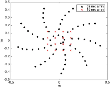
Figure 4 – Two different arrays geometry. 62-microphones in log-spiral configuration (black dots) and Rectangular 16-mics configuration (red crosses).
To understand why, one could make a mathematical analogy with linear systems,
suppose a linear system with transfer function such as:
H(f) =1
in a way that impulse outputs remain equal to their inputs. In other words, an ideal array
would have a PSF equivalent to this transfer function, so that the final image due to a source
point would be exact only this source point, i.e., the system’s output remains the same as
the input. For more details about linear systems (13–15). Nonetheless, consider a transfer
functionH(f)for an ideal low-pass filter (also called as sinc filter) instead of an unit gain,
H(f) =r e c t( f
2B) whereBis an arbitrary cutoff frequency (or bandwidth).
If an impulseδ(t)is applied to it, the output is
h(t) =F−1{H(f)}=2Bs i n(2⇡B t)
2⇡B t =2B s i n c(2B t).
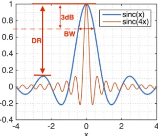
Figure 5 – Two different plots for thes i n c(.)function that can be further associated with a PSF map. Beamwidth (BW) and dynamic range (DR) are indicated for performance measurements.
Fig. 5 shows a typical plot for a sinc response. The PSF map has a form similar to a
sinc function, even though it is three-dimensional, as in Fig. 6. The bandwidth limitation
(above cited) can then be seen as array limitation specifically the finite aperture (spatial
extent) of the limited number of microphones.
For example, the two functionss i n c(x)ands i n c(4x)in Fig. 5 would represent the
PSF response of two different arrays. The one with more sensors and bigger aperture would
have its PSF represented bys i n c(4x)corresponding to a narrow beamwidth and lower side
lobes level. By contrast, smaller configurations with fewer sensors would be represented by
s i n c(x).
Thus, the point-spread function is commonly used to see how a point source reveals
itself within the array. This is commonly used to measure the array’s performance in terms
of beamwidth (BW) and sidelobe levels (or dynamic range - DR) in Fig. 5. A narrow beam
Figure 6 – PSF for the 62-mic antenna shown in Fig. 4 at 8 kHz and 1 m away revealing the similarity with the sync functions depicted in Fig. 5.
To represent the PSF map, a point source can be modeled in terms of radiation
directivity, as a monopole or a dipole. In this particualr study, point sources are going to be
treated as dipoles, as done by Lowis (2) and Sitjsma (16). The effect of a dipole stationary
tonal source, denoted ~j, was simulated following the guidelines provided by Sijtsma (16).
This source induces a CSM given by
Cj =g~Hj g~j =w~jHw~j (1.35)
wherew~ is the steering vector for unit power source. The beamforming map is obtained by scanning the grid points⇠s leading to
bj s=w~sCjw~sH =w~s(w~jHw~j)w~sH =||w~sw~Hj ||
2 (1.36)
which means that the PSF map can be obtained by fixing the steering vectorw~j at the source
position while sweepingw~s over the image mesh grid⇠s. As an example, Fig. 7 shows a
16-mic array (blue circles) and an arbitrary mesh located 1 m away (black dots). The sweeping
is made over this fixed mesh.
For the free-field case and the arrays in Fig. 4, the PSF maps are presented in Fig.
Figure 7 – 16-mic array (blue circles) and an arbitrary 25 by 25 points mesh (black dots).
16-mic, has a much wider beam (top plots) in comparison to the 62-mic (bottom plots).
Besides, it is possible to see an aliasing process happening for the top-right plot, i.e., the
repetition of the main lobe periodically in the space. This phenomenais similar to the
Nyquistcriteria(14) and because of the array limitation, there is a limited region in the
space that the beamforming can sweep. Outside of this region, a periodic repetition of the
main lobe appears and consequently leads to noise sources that appear in the map where
in fact no source is physically present.
The formulation presented above is independent of the steering vector formulation.
We already introduced PSF maps for the free-field case (Fig. 8). Regarding the Eq. 1.23 for
the modal steering vector, the duct PSF can also be performed in order to visualize its effects
within the duct.
For the USP fan rig geometry, a simulation example can be applied in Fig. 9 for a
source located atr =0.15m,✓ =0 andz=−0.71m. This focal plane (fp), thez distance, is the same of the fan plane. Frequencies in the range between the 1st and 4th BPF equivalent
for 4250 RPM were evaluated. The USP array and rig geometry are detailed in Chapter 3.
It is important to mention that, due to the small number of modes at low frequencies,
Figure 8 – PSF for the arrays on Fig. 4 at two frequencies: 2 and 8 kHz. Source 1 m away. Top maps regard the 16-mic array and bottom maps, the 62-mic array.
has a large main lobe. At 1.13k H za clearly discernible source close to the wall is observed
and comprises only 11 cut-on modes. Strong beamforming side-lobes can also be seen.
At higher frequencies source discernibility increases followed by diminished side-lobes
confirming code plausibility.
For the ANCF rig at NASA, results for PSF can also be applied. The NASA array
(detailed also in Chapter 3) has many more microphones (around 90) as compared to the
USP fan rig’s 77 mics. As already discussed, better performance is expected for this array
Figure 9 – PSF for the duct steering vector formulation. USP fan rig configuration for duct-radius and focal plane distance. Frequencies are evaluated from the 1s t to the 4t hBPF equivalent for a 4250 RPM shaft speed.
1.4 DUCT MODES ANALYSIS
Unfortunately no references for modal analysis were found in the literature. Dougherty
shows good results for modal analysis in (3) and (5) but it is unclear how to perform them.
Close inspection of equations 1.21 and 1.23 reveals thatgi can be re-written in a
double sum involving circumferential and radial modes(m,n)
g =X
m X
n
gm,n (1.37)
Figure 10 – PSF for the duct steering vector formulation. ANCF-NASA fan rig configuration for duct-radius and focal plane distance. Frequencies are evaluated from the 1s t to the 4t hBPF equivalent for a 2029 RPM shaft speed.
broken into modes:
Bmodes= 2 6 6 6 6 6 6 4
g1,0
g1,1
.. .
gm,n 3 7 7 7 7 7 7 5
C⇥gH1,0gH1,1···gHm,n⇤=
2 6 6 6 6 6 6 4
g1,0CgH1,0 g1,0CgH1,1 ··· g1,0CgHm,n
g1,1CgH1,0 g1,1CgH1,1 ··· g1,1CgHm,n
..
. ... ... ...
gm,nCgH1,0 gm,nCgH1,1 ··· gm,nCgHm,n 3 7 7 7 7 7 7 5 . (1.38)
Bearing this in mind and taking another perspective: if the steering vector is a linear
combination of several modal steering vectors, like in Eq. 1.37, and if we take for example,
only 3 steering vectors, it becomes
substituting this in Eq. 1.7 we have
b1= (g1+g2+g3)C(g1+g2+g3)H
b1= (g1+g2+g3)C(gH1 +g H 2 +g
H
3) (1.40)
and opening the sum we have
b1=g1CgH1 +g1CgH2 +g1Cg3H+g2CgH1 +g2CgH2 +g2CgH3...
+g3CgH1 +g3CgH2 +g3CgH3. (1.41)
However, if we think of beamforming as a linear operator, sinceT[u+v] =T[u]+T[v]
whereu andvare arbitrary vectors andT[·]is an arbitrary linear operator, the beamforming output as a result of a sum of steering vectors would give
b2=g1CgH1 +g2CgH2 +g3CgH3. (1.42)
Clearly Eqs. 1.41 and 1.42 are not the same. The solution adopted was consider
that in fact the beamforming process is a linear combination of every single modal
beam-forming map, i.e., the final beambeam-forming map can be generated by a double sum of(m,n)
beamformings map for each single mode.
As a consequence, assuming modes mutually orthogonal implies that the elements
ofBmodesaway from the main diagonal are theoretically zero, suggesting that duct beam-forming reduces to a double sum of(m,n)independent beamforming maps, one for each
singular modal steering vector. Acoustic mode by mode maps may be computed together
with their allied singular mode power at each frequency obtained by integration over each
2 SIGNAL PROCESSING TECHNIQUES
Chapter 1 described all the necessary background theory to compute the correct
steering vector for the duct-beamforming technique. Moreover, some concepts like mode
propagation within ducts were also introduced.
For the free-field case and spatially stationary sources, the computation of the
cross-spectral density matrix can be directly estimated. However, to obtain the cross-cross-spectral
density matrix correctly for fan noise analysis, signal processing techniques are required.
They include fan harmonic tone removal, the use of virtual rotating microphones; data
sampling rate changes and last but not least, adequate spectral estimation. A brief review of
the techniques employed here are described next.
2.1 TONE REMOVAL
A spinning fan (or a propeller for that matter) generates strong harmonic tones
referred to theblade passing frequenciesor BPF. This phenomenon is due to the periodicity
of the blades’ wake in the flow. The frequency is easily calculated by fB P F =ff a n(R P M)⇤B/60, whereff a n(R P M)is the fan speed in RPM andB the number of blades. These tones can be strong enough to allow power leakage onto the estimated spectrum, leading to estimation
errors in both magnitude and phase. For the sake of beamforming imaging, it is important
to remove those tones from the signal prior to PSD estimation.
To do so the approach used here rests on subtracting a synthesized harmonic
se-quence from the total signal, i.e., after estimating the allied amplitudes/phases for each
harmonic sinusoid, the estimated signal is subtracted from the measurements in the time
domain. This contrasts with a commonly adopted practical alternative that processes the
data in the frequency domain by averaging the tone peak along its neighboring values,
leading to less desirable results.
Consider a signalx(n),n= [1,...,L]composed by a sinusoidal with a known frequency
x(n) =As i n(2⇡n f0+φ) +e(n)
or equavalently
x(n) =A0c o s(2⇡n f0) +B0s i n(2⇡n f0) +e(n) (2.1)
where
A0=As i n(φ) a n d B0=Ac o s(φ)
Rearranging Eq. 2.1 in the matrix form we have
2 6 6 6 6 6 6 4
c o s(2⇡f0) s i n(2⇡f0) c o s(2⇡.2f0) s i n(2⇡.2f0)
...
cos(2⇡.L f0) s i n(2⇡.L f0) 3 7 7 7 7 7 7 5 2 4 A0 B0 3 5= 2 6 6 6 6 6 6 4
x(1)
x(2)
... x(L)
3 7 7 7 7 7 7 5 + 2 6 6 6 6 6 6 4
e(1)
e(2)
... e(L)
3 7 7 7 7 7 7 5 (2.2) or C 2 4 A0 B0 3
5=x+e
The optimal solution that minimizeseHe, the sum of squared errors, is given by
2 4 ˆ A0 ˆ B0 3
5= (CTC)−1CTx (2.3)
where(CTC)−1CT is the pseudo-inverse of the matrixC.
The pure tone
C 2 4 ˆ A0 ˆ B0 3 5
is then subtracted from the raw signalx(n), so the tone free signal ˜x(n)is computed by
˜
x=x−C
This formulation presumes that the frequencyf0is well known. To invoke this
ap-proach, a high degree of certainty in the f0value (error less than 0.1%) is necessary.
To overcome this problem, consider the first estimation of the BPF coming from the
fan speed displayed in the monitoring system during the experiment. For example, 4000
RPM. For a 16 bladed rotor, it will produce a 4000⇤16/60=1.067k H z BPF.
A second and better estimation of this frequency can be obtained by a measured
acoustic pressure data from one microphone. A long data set, in this work 216samples, is
Fourier transformed and, once in frequency domain, a range of frequencies close to the first
BPF is selected and the maximum value of this segment is registered. This maximum value
is associated with the first BPF.
In this way, this value gives a second estimation for the frequency f0. Surely an
improved estimation although not yet good enough.
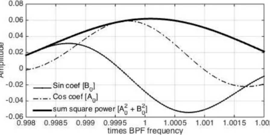
Figure 11 – CoefficientsA0andB0of Eq. 2.3 and the squareA20+B02for an aleatory experiment with fan noise data.
This second estimation offB P F is used to apply the tone removal introduced above.
However, the procedure is repeated about 100 to 150 times around±0.2% of fB P F. The
algorithm performs this search and look for the maximum coefficients of square sines and
cosines of Eq. 2.3, i.e., look form a x{A20+B02}. The maximum is obtained when the frequency
matches the real fB P F generated by the fan. A result for this search can be seen in Fig. 11
where the maximum in the power of coefficients is clearly visible.
This maximum is then used as the exactfB P F necessary to remove all tones from all
microphone signals. The procedure is repeated until the desired order of BPF. In this work,
2.2 VIRTUAL ROTATING MICROPHONES - VRM
As introduced in Chapter 1 rotating beamforming requires a rotating reference frame
for the formulation of the steering vector. Moreover, the signals from microphones must be
spinning at that same speed. Certainly it is not feasible to make microphones spin with the
fan. Fortunately, there are some techniques that make the microphones spin virtually, by
measurements from microphones at rest.
There are two known different ways to achieve this. It is possible to employvirtual
rotating microphonesas explained by Lowis in (2) and by Pannertet al.in (17). The technique
proposed by them relies on the frequency shift caused onto the spinning modes.
Briefly, the signal from a ring of microphones is transformed from the time domain
to the mode domain, via a spatial Fourier transform. Thus, one can obtain the corrected
frequency (shifted) to the corresponding in the rotating frame in frequency domain on a
mode by mode basis:!+mΩ.
After this correction, the inverse spatial Fourier transform is carried out resulting in
the signals of virtually spinning microphones at velocityΩ. Lowis and Pannert demonstrated
that this has same effect as if the microphones were rotating around the duct axis at same
speed as the fan.
The latter technique was not employed in the present study. For convenience, we
opted for using the interpolation technique as described by Herold in (18). A brief
introduc-tion of the method is presented as follows, but intuitively it is equivalent to stroboscopically
sampling the signals.
The principle behind the interpolation technique consists in creating virtual
mi-crophone measurements (i.e., physically do not exist) from static measurements recorded
in the circular array. If we fix a rotating point with same speed and direction as the fan,
the interpolated sound pressure at this point in a certain time will be the average of the
neighboring microphones in the wall-mounted array, weighted by its angular spacing from
that point to the microphones, just as a linear interpolation.
Mathematically speaking, letNc be the number of equally spaced microphones on
The angle↵between each microphone is given by↵=2⇡/Nc.
If we define the time-dependent angle of the measured point '(t) by the angle
position from some reference point in the rotating frame at speedΩ, the limit index, lower
and upper (ml andmu respectively) of the static microphone signals in which we can
interpolate is calculated by
ml(m,t) = ö
m+'(t)
↵ −1
ù
m o d Nc +1 (2.5a)
mu(m,t) = ö
m+'(t)
↵
ù
m o d Nc +1 (2.5b)
whereb·cdenotes the floor function and “mod” is the congruence operator. Thus, the weight-ing factors for the respective sound pressures are given by
su(t) =
'(t)
↵ −
ö'(t)
↵
ù
(2.6a)
sl(t) =1−su(t) (2.6b)
Finally, the interpolated microphone signalspΩ,m in the rotating frame are calculated
by
pΩ,m(t) =slpml+supmu (2.7)
Once calculated, the virtual rotating signalpΩ,m(t)is then synchronized with same
speed with respect to the fan about an axis of interest. The CSM for the virtual rotating array
is then estimated equivalently to the stationary case from thepΩ,m(t)signals.
2.3 DATA RESAMPLING
Ideally, the best way to acquire acoustic data for fan noise analysis is a data
acquisi-tion system triggered to the fan speed via an encoder attached to the shaft (4). Many acoustic
on the shaft speed, i.e., most of noise sources are frequency multiples of the shaft speed,
hence, the BPF.
In this way, if the data is acquired synchronously with the shaft speed, for example
512 samples per fan revolution, the frequencies of these sources correspond exactly in the
estimated spectral bins, if used as usual a power of 2 data tapper.
But, if no shaft-sync data acquisition is available, data resampling can be performed
to simulate the same effect. This is done in order to give an exact number of samples per
revolution. In this work, for convenience, that data was resampled to give 512 samples per
fan revolution. To do so a sensor attached to the shaft was used to provide 1 pulse per fan
revolution.
Furthermore, when the PSD is estimated from data synced with the fan speed, for a
given data window length, the BPF harmonics always match the same bins in the frequency
axis. For example, given a 2048 sample data window and 512 samples per revolution sample
rate, the PSD’s frequency axis (with 1024 bins from 0 tof s/2 where f s is the sample rate,
f s =512⇤shaftspeed) always has in the(64+1)t hposition for the 1s t BPF,(128+1)t h position
corresponds to 2n d BPF and so on.
2.4 POWER SPECTRAL DENSITY (PSD) ESTIMATION
The beamforming technique relies directly on PSD estimation, which is an
impor-tant preliminary step to achieve the final acoustic map. Pressure signals coming from all
microphones in the array are processed to produce the cross-spectral density where from
beamforming can be computed. One must, however, keep in mind the several practical
limitations of spectral estimation methods that vary according to the signal characteristics
that lead to like power leakage, spectral blurring, bias, and so on (13–15).
Aeroacoustic noise signals (19) possess continuous spectra derived due to their
nature as regular stochastic processes, i.e. without strictly sinusoidal tones. This is in contrast
to problems, for example, regarding the electrical power networks whose signals are mostly
comprised of 60 Hz and its harmonics.
acquired data. It allows for the comfortable use of the well known Welch spectral estimation
method (14), in which, as is customary in the literature (13), to adopt 50 % of overlap between
signal segments before averaging the absolute squared value of the transforms for each
data subsegment to obtain the spectral density estimate. The Hanning window (14, 19) was
used throughout, as it is the most popular data window due to its good trade-off between
main-lobe aperture and reduced side-lobe levels.
On applying windows in the case of continuous spectra, careful normalization is
required to ensure that the power computed over time is the same as the one that would be
obtained integrating the spectrum. If the spectrum contains pure sinusoids, the required
normalization is different from that of a continuous spectrum leading to some
prevail-ing confusion (20). Because BPFs were extracted from the data, we strictly employed the
continuous spectral data window normalization here.
2.4.1
PSD Estimation Details
Let two data records of two signalsxandyof length comprisingN samples, be broken into blocksx(k)andy(k)of sizeL
ˆ
Sx y(k)(f) =2· F(x
(k)·w)·c o n j(F(y(k)·w))
P
wi2 (2.8)
wherew= [w1...wi...wL]T is a suitable data taper window of lengthL(usually Hanning
window (19)). The symbolF {·}stands for the discrete time Fourier transform computed at suitable frequencies f between 0 and one half the Nyquist frequency. The factor 2 comes
from using a single-sided representation (positive frequencies only) of the spectrum.
Finally, the cross-spectrum is given by averaging the terms in
ˆ
Sx y(f) = N/L X
k=1
ˆ S(k)
x y
N/L (2.9)
For the cross-spectral matrix, all pairwise microphone combinations must be
by
⇥ C(f0)
⇤ N x N =
2
6 6 6 6 6 6 4
S11(f0) S12(f0) ··· S1N(f0) S21(f0) S22(f0) ··· S2N(f0)
... ... ... ...
SN1(f0) SN2(f0) ··· SN N(f0) 3
7 7 7 7 7 7 5
N x N
. (2.10)
The term position is used because the CSM is three-dimensional with size[N x N x(L/2)], whereLis the data taper length. Commonly the depth of this matrix corresponds to one
frequency, and a position of[N x N]will have all microphones cross-spectra combinations
3 EXPERIMENTAL SETUP
This study used two different experimental setups for analysis and comparisons: one
constructed at the University of São Paulo, at the São Carlos campus and the ANCF rig at the
NASA-Glenn Research Center - USA whose use was was granted via a research partnership
between USP and NASA-Glenn allowing data exchange and access to technical details.
This section describes the specifications of both fan rigs.
3.1 UNIVERSITY OF SÃO PAULO (USP) FAN RIG TEST
FACIL-ITY
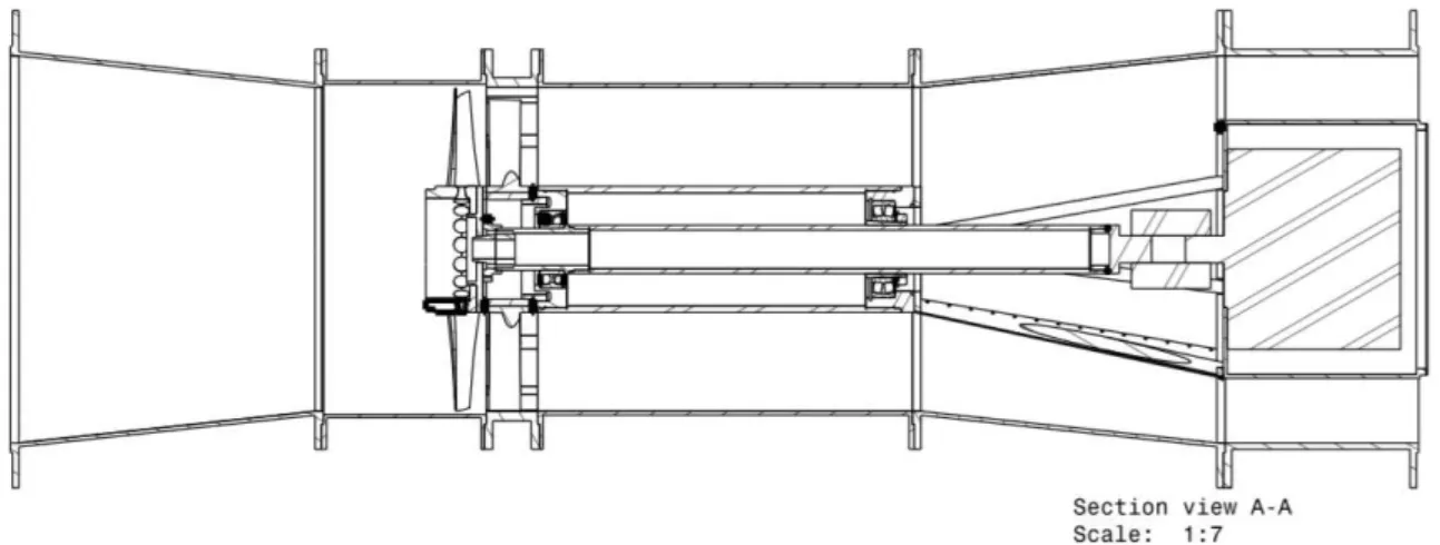
Figure 12 – Motor section details.
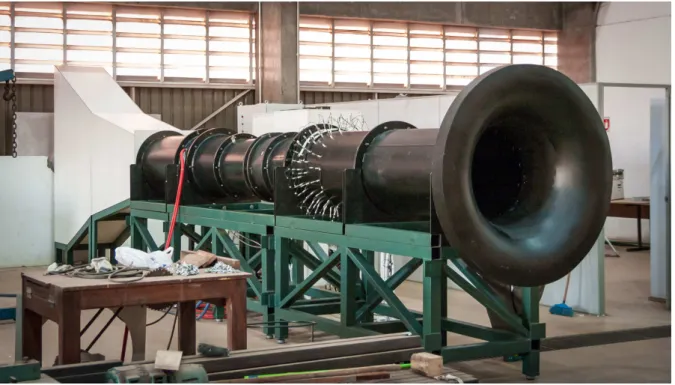
The USP rig is a long-duct low-speed fan rig test facility constructed to provide
a means for experimentally studying the fluid dynamic details of fan noise generation
mechanisms. The rig’s configuration was designed with flexibility in mind and allows rig
section replacement to suit specific experimental needs.
The rig has a diameter 0.6 m and is about 12 m long; its basic configuration comprises
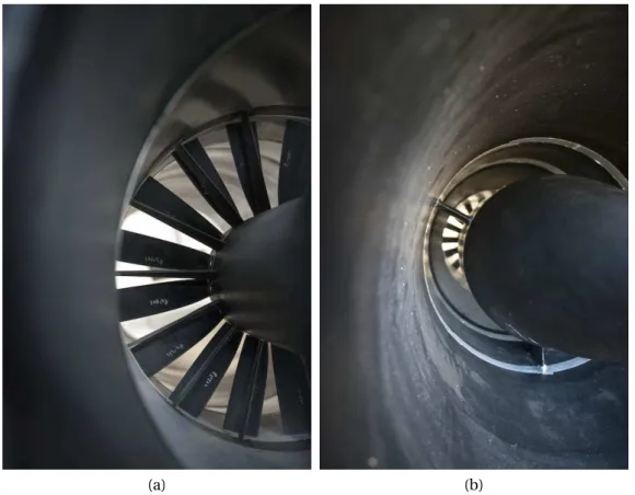
a 0.5 m diameter duct fan stage equipped with a 16-bladed rotor and a 14-vaned stator, as
depicted in Figs. 12, 13, 14, 15 and 16. The rotor is powered by an 100HP electrical motor
Figure 13 – USP fan rig. Overall view with anechoic termination and bell-mouth inlet.
Figure 14 – Details of the 0.5 m diameter rotor.
speed. Its long duct configuration is similar to that of DLR low speed fan rig (21) and yet
differs from other rigs that operate inside anechoic chambers (4, 6, 22).
3.1.1
Antenna design
Microphone duct-array design must take into account some important aspects,
namely: bandwidth; distance from the focal plane; duct diameter; number of sensors;
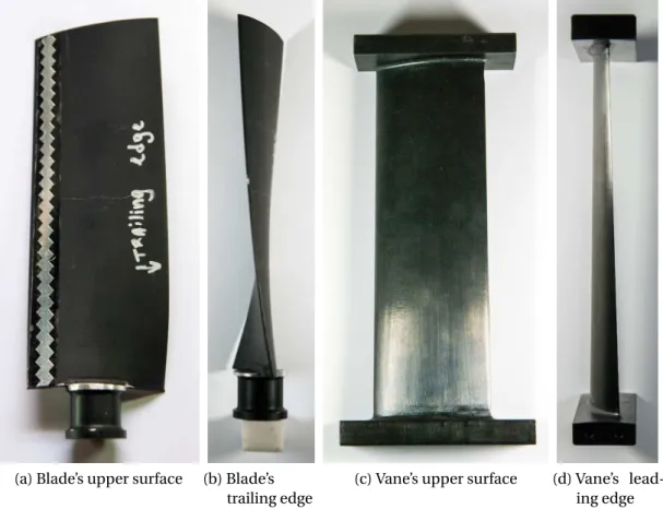
(a) 14-vaned stator (b) 16-bladed rotor
Figure 15 – Details of the pair rotor and stator used in the USP fan rig.
be used as guidelines. Notable exceptions are represented by (2, 4, 6).
It is known that the total length of the array directly influences the PSF beam-width
and side-lobes. Longer arrays have better focus-depth relationship at the expense of a loss
in coherence between rings. This calls for a trade-off that must be sought for this array
parameter.
The number of microphones per ring depends directly on the maximum
circumferential-mode order of interest, according to the Nyquist criteria:−Nc/2+1<m✓ <Nc/2−1, where Nc is the number of microphones in the ring andm✓ the maximum circumferential-mode
order that the array is able to detect without aliasing. Furthermore, Tyler-Sofrin modes can
be used as reference to predict the highest order mode as a function of the number of fan
blades and stator vanes.
The first big issue in this project was to design the optimal array geometry for rotating
beamforming and mode detection. The first attempted configuration was a 4-ring one,
comprising 16 mics each, as seen in Fig. 18. We believed that, with a longer array, more rings
and fewer microphones per ring, we could increase the array’s capability to distinguish close
sources, i.e., its beam width would be smaller. However, Lowis (2) has shown that optimal
(a) (b)
Figure 16 – Backside view: (a) Close-up in the rotor-stator stage and (b) the end of the rotor stage with 3 struts supporting the motor and the aerodynamic termination.
(around 100). In fact, it is far more important to have a minimum number of sensors per
ring (in this case, more than 20 sensors per ring) than to have a large number of rings.
In the first array (see Fig. 18) theoretically only modes up tom=±7 could be detected which is insufficient for reasonable characterization of fan broadband noise. Furthermore,
beamforming map artifacts occur in a circumferentially symmetric pattern that is a multiple
of the number of sensors at each ring. So, for a fan with 16 blades and an array with 16
sensors per ring, artifacts with a 16 pattern would be undesirably jumbled with a possible
noise coming from the blades.
For these reasons a second version of the microphone array was introduced. The
solution was to reduce the number of rings and increase the number of sensors per ring. The
total array length went from 0.42 m to 0.27 m in the final array version and an odd number
of microphones was used per ring. This last solution was adopted to avoid artifacts in the
form of multiples of the number blades on the beamforming map and to allow the easy
Finally, as the number available of microphones was limited, each ring was endowed
with a different number of microphones. A ring with larger number of sensors closer to the
focal plane is highly recommended to facilitate the detection of higher order modes.
Moreover, (5) observed that aligned microphone pairs were far more correlated than
pairs corresponding to different angles. It is believed that the cause is convected boundary
layer turbulence: two microphones experience nearly the same turbulence if they are aligned
stream-wise leading to a rule aligned microphone designs should be avoided. Also the use
of different numbers of microphones per ring contributes to avoid the repetition of the
distances between microphones much like in non-periodic plane arrays (23).
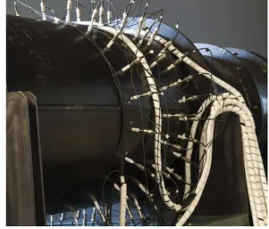
Fig. 19 shows the second array designed. It has three separate rings 0.10 and 0.17 m
apart, each ring comprising 33, 23 and 21 uniformly distributed microphones.
(a) Blade’s upper surface (b) Blade’s trailing edge
(c) Vane’s upper surface (d) Vane’s lead-ing edge
(a) 64-mic array (circles) and the focal plane represented by the black dots.
(b) Microphones mounted.
Figure 18 – First antenna used with 4-rings and 64-microphones.
(a) 77-mic array (circles) and the focal plane represented by the black dots.
(b) Microphones mounted.
Figure 19 – Second antenna composed by 3-rings with 77-microphones in total.
3.1.2
Acoustic data acquisition system
The acoustic data acquisition system comprises flush-mounted microphones (GRAS
40PH-S2φ7m m, bandwidth of 20 to 20k H zand 50m V/P a average sensitivity) operated via a PXI National Instruments system composed of 5 PXI-4496 boards. Angular motor
3.1.3
Blade trip strip
Following (24) section 7.3: “A more complex form of lock-in that can occur in
low-speed fans is calledlaminar boundary layer-wake interaction.Qualitatively speaking,
pe-riodic shear layer velocity perturbations, due to Tollmein-Schlichting waves and hairpin
vortices, occur during the transition from laminar-to-turbulent boundary layer flow on rotor
blades when the Reynolds number based on the chord length is in the approximate range
105 <U C/⌫ < 106, whereU is the velocity at the leading edge of the blade. If the frequency
of these periodic shear layer instabilities matches the frequency of vortex shedding, then a
hydrodynamic lock-in phenomenon takes place. This causes the periodicity in the wake of
the blade to be amplified. If these vortex frequencies happen to be near a harmonic of the
BPF, then significant increases in the sound at this frequency will occur.” Since the USP fan
rig operates in a similar situation, a trip strip was used to force the shear layer transition
from laminar to turbulent at the same blade position. Without the boundary layer trip strips
the shape of the blade wakes (depth and width) varied significantly from blade to blade.
This caused the energy to change from BPF to lower shaft orders and into the broadband.
The necessary trip length was estimated using Pope (25) as reference. Calculations
are highlighted on Table 1.
3.2 ADVANCED NOISE CONTROL FAN - ANCF - NASA GLENN
Data from a second fan rig test facility was used to perform algorithm validation
and for result comparison. The ANCF at NASA Glenn is a short-duct low-speed fan rig as
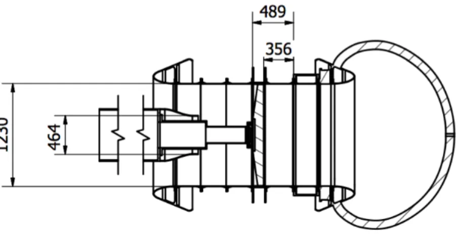
described in (22) and (26). It is 1.22 m in diameter. The hub is 0.457 m at the fan and 0.61 m
aft portion of the duct, as shown in Figs. 20, 21 and 22. The rotor and the stator have the
same geometry and blade/vane count as the USP fan rig even though the ANCF is larger. It
is powered by an electrical motor fixed outside the duct allowing it to achieve speeds up to
2000 RPM and Mach 0.13 mean axial flow speeds.
The 90-microphone duct-array has 3 rings of 30 sensors equally spaced upstream
micro-Table 1 – Fan rig parameters for trip-strip height estimation
Meters Imperial (Feet)
1 m to 1 3.28
Blade chord 0.057 0.187
Blade span 0.25 0.82
Speed (RPM) 4250 4250
Speed (70% span) 77.9 m/s 256 feet/s
Sound speed 355 1164
Mach# @blade 0.17 0.17
Air flow 60.4 198
U total(70% span) 98.5 323
Air kin. Visc. 15.7µ 169µ
Reynolds 358k 358k
Re effective 6.28M 1.92M
LE-to-trip (%Chord) 5% 5%
Re (LE-to-trip) 17.9k 17.9k
Constant K — 1000
trip height 0.16mm 6.26mInch
phones in the radial direction placed just on the inlet. The rake spins at 1/100t hthe speed of the fan and is used for mode detection.
Figure 20 – ANCF technical draw. Units in mm
In Fig. 21 the duct inlet is hidden behind theinlet control device(ICD). The first blue
section after that, contains a 90-microphone array. Downstream, the gray section there
are 2 rings of 16 speakers each surrounding the duct. These speakers are used to generate
Figure 21 – ANCF: side view. Inlet hidden by the ICD. Microphones array in the downstream section after the ICD followed by the duct-speakers section for artificial noise generation.