FUNDAÇÃO GETULIO VARGAS
EPGE
Escola de Pós-Graduação em Economia
"Measuring core inflation as the
common trend of prices"
Prof. Antonio Fiorencio
(IBMEC)
LOCAL
'. . Fundação Getulio Vargas
Praia de Botafogo, 190 - 10° andar - Auditório Eugênio Gudin DATA
26/1012000 (5a feira)
HORÁRIO 16:00h
Measuring core inflation as the common trend of prices*
Antonio Fiorencio I
Ajax R. Bello Moreira2
May2000
Abstract: In recent years, many central banks have adopted inflation targeting policies starting an intense debate about which measure of inflation to adopt. The literature on core inflation has tried to develop indicators of inflation which would respond only to "significant" changes in inflation. This paper defines a measure of core inflation as the common trend of prices in a multivariate dynamic model, that has, by construction, three properties: it filters idiosyncratic and transitory macro noises, and it leads the future leveI of headline inflation. We also show that the popular trimmed mean estimator of core inflation could be regarded as a proxy for the ideal GLS estimator for heteroskedastic data. We employ an asymmetric trimmed mean estimator to take account of possible skewness of the distribution, and we obtain an unconditional measure of core inflation.
1. Introduction
In recent years, many central banks have adopted inflation targeting policies starting an intense debate about which measure of inflation to adopt. Thjs debate reflects the suspicion that standard inflation indexes might give a misleading picture of the "real" leveI of inflation. Standard indexes might be toa ''nervous'' in the sense of not discriminating (i) idiosyncratic from generalised price shocks and (ii) temporary from permanent shocks. If this is so, the conduct of monetary policy would be obviously impaired.
The literature on core inflation has tried to develop "less nervous" indicators of inflation which would respond only to "significant" changes in inflation. Many altemative approaches have been proposed and all of them are concemed with noise filtering. But the definitions of what is noise do
• Authors thank Ingreed Valdez, Marina Paes and Leonardo de Carvalho for research assistance and Eustaquio Reis, João Victor Issler and Hélio Migon for useful comments on an earlier version ofthis paper.
1 Faculdades Ibmec, [email protected]
differ, reflecting a lack of consensus about what should be measured and why
not use standard indexes 1
•
Since the literature on core inflation has been largely motivated by the literature on inflation targeting, it wiIl be useful to consider the relationship between them.
An inflation targeting regime requires two different measures of inflation. The first measure is the inflation target itself, which defines policy objectives and might help co-ordinating agents' expectations. The target must be credible, easily understandable and its history should not change as new information arrives - conditions that would not be met if the target were defined in terms of an econometric model.
The second measure of inflation is the core inflation which shows
inflation trends over the' short-run and, thus, whether policy is on track. It is
not necessary that the "core" possesses the same characteristics of the "target". Rather, it must reflect effective changes in inflation: (i) it should
discriminate between idiosyncratic and generalised movements in prices; (ii)
it should discriminate between temporary and persistent movements in prices; and (iii) it should lead the probable short-run trend of inflation. (The literature frequent1y assumes that the indicator should discriminate supply from demand shocks. This is not so obvious for us and we will not require this ability from the indicator. We are interested on movements in inflation, whatever their
sources2
.)
These are not arbitrary characteristics. Without such an indicator it is more probable that monetary policy wiIl be highly volatile since it wiIl be continuously reacting to noise and wiIl not be pre-emptive. Thus, the key words for us are: generality, persistency and lead-power.
Targets and Core are different things but the literature tends to treat them as one. In this paper we are interest on core inflation exclusively as an indicator ofinflation or, more to the point, as an indicator ofwhether policy is on track. This means that the definition of the indicator wiIl depend on the
1 "Surprisingly, precise definitions of [core inflation] are rarely provided." (Bryan & Cecchetti (1999), pg 1)
"In general, core inflation tends to be defmed in terms of the particular method used to construct a practical measure rather than in terms ofwhat the measure is trying to capture." (Roger (1998), pg 1)
"I evaluate the competing merits of the ditTerent approaches [to measure core inflation], and argue that a common shortcoming is the absence of a well-formulated theory of what these measures of inflation are supposed to be capturing." Wyne (1999, pg 2)
2 "At the Fed, I can assure you, we never thought ofthe exchange rate as a source of 'noise'. Far from being
definition of the target. Many different indexes might serve as the basis for
the target: consumer price indexes, wholesale price indexes etc. But, once the
target has been defined, the indicator should suggest whether policy
conceming that target is on track. In 1999 Brazil moved to an inflation target
regime where the target inflation rate is the IPCA3• So, for us, core inflation
will mean core IPCA 4•
Section 2 briefly reviews the existing approaches to measuring core inflation. Section 3 presents our measure of core inflation and section 4 considers whether this measure is an effective lead of the corresponding headline indexo Section 5 conc1udes.
2. The maio approaches io the Iiterature
The literature presents four main approaches to compute core inflation5
•
(i) The most traditional approach is the "ex. food and energy". This amounts to pre-specifying a fixed group of products that will be systematically exc1uded from the computation of the inflation core. The reason for the exc1usion is usually the fact that the prices of these products are "too volatile". But since relative volatilities can. change, you must be
somewhat prescient to employ this approach effectively. In fact, there is not
much to be said in favour of this approach except that it is simple.
(ii) By far, the most popular current approach to compute core inflation are the trimmed estimators proposed most notably by Bryan and Cecchetti in
several papers6• The problem is the following. Price indexes are an average of
individual prices. If the distribution of prices at a given moment were normal,
the arithmetic mean of observed prices would be an efficient estimator of the general price leveI. There is, however, reasonable intemational evidence that the cross-sectional distribution ofprices is not normal, rather, it appears to be asymmetric and leptokurtic (fat tailsY. If the distribution is leptokurtic, the literature recommends trimming the sample to estimate the mean, which produces an improvement in the efficiency ofthe estimator.
3 IPCA (Índice de Preços ao Consumidor Ampliado) is a consumer price indexo
4 We will not discuss traditional sources ofbias in consumer price indexes such as quality and substitution
bias.
5 We present the main issues brief1y. For more complete reviews the reader may consult Roger (1998) or
Wyne (1999).
6 See the bibliography.
7 Menu-costs are a possible rationalisation of these characteristics, but the trimming approach does not depend
The main criticism to the trimming approach is that it is not obvious how to compute the optimal amount of trimming and approximate measures might not be robust8
•
(iii) Trimmed estimators can deal with the problem of efficiency but they do not address the problem of discriminating permanent form transitory shocks. Dealing with the persistence issue leads to the third approach: smoothing. Cogley (1998) suggests employing an exponentially smoothing filter.
This procedure will filter away temporary shocks and give a better idea of the current inflation trend, but it does not address the problem of efficiency mentioned before.
(iv) None ofthe above approaches makes much useof economic theory to define core inflation. Quah and Vahey (1995) use the structural vector autoregression approach to construct measures of core inflation that draws on economic theory. They estimate a bi-variate V AR consisting of inflation and output and they define core inflation as the component of inflation that has no long-run impact on output.
One problem with this approach is that identifying assumptions are always debatable. For instance, the idea that in the long run the price leveI does not affect output would probably be much less debatable than Quah and V ahey' s hypothesis that inflation does not affect output in the long run9
•
3. The common trend model
The main hypothesis behind our approach, and probably behind the other measures of core inflation, is that price changes of all products share one common trend, which is the "real" inflation leveI 10. However, this
common trend cannot be direct1y observed due to idiosyncratic product price fluctuations and transitory macro fluctuations.
The markets for each product react to macro and specific shocks and the resulting price fluctuations can be decomposed into two parts. The first is common to all products and the other is specific to each product. The latter
8 See Bakhshi and Yates (1999).
9 Wyne (1999) also makes this point. Blix (1995) assumes that the priee leveI does not affeet output in the
long-run.
\O More than one trend ofpriee ehanges ean only be justified by improbable persistent relative produetivity
reflects the specific conditions of each market - such as the price elasticity to supply and demand shocks, or, maybe, the costs of price adjustment - and should be discarded from the core inflation measure. Notice that, since market characteristics differ, there is no reason to expect that the idiosyncratic
components wiIl share the same distribution. In particular, the distribution of
their standard deviations might be quite dispersed.
Even if we eliminate the idiosyncratic components, there is stiIl the problem that macro shocks could have transitory as weIl as persistent effects on inflation. Common movements of products' prices can be decomposed into one component that wiIl disappear within one period, and another one that wiIl persist for the foIlowing periods. Since the first component wiIl disappear fast, it should not affect long run expectations or outcomes and, thus, it should be discarded from the core inflation measure.
FinaIly, monetary authorities can only affect the future leveI of inflation and their actions must be pre-emptive. If they are to react to what is likely to happen instead of to what has already happened, the core must lead the near future leveI of inflation.
Thus, our measure of core inflation should have three properties: (a) it should estimate general or common price fluctuations·discarding idiosyncratic
product price fluctuations; (b) it should estimate only persistent11 price
movements discarding transitory macroeconomic effects; and (c) it should lead the future leveI of inflation.
Core inflation, as defined by (a) and (b), can be related to the common trend (!lt) of product prices (1tit) measured by the foIlowing dynamic muItivariate model where the errors are heteroskedastic.
i=l. .. N (1)
çt -(O,W)
In this model, idiosyncratic noises are represented by (eit) which has
specific volatility ( 。セIL@ and the macro transitory component is represented by
(çtY2. The model was estimated using monthly data for the period [July 1994,
11 It is important to draw the distinction between persistent and pennanent shocks to inflation, but it may be
empiricaIly difficult to estimate both shocks with any precision, speciaIly in smaIl samples like ours which contains on1y about 60 observations. In this paper we will be concemed on1y with pennanent shocks and we wiIl ignore persistent shocks.
12 Representing the idiosyncratic and macro transitory components as non correlated noises is the simplest way
January 2000]. This is a very short sample but previous data can not be used
since price dynamics in Brazil changed with the Real Plan of 199413
•
This model cannot be estimated using standard procedures. First, the
dependent variable space dimension is very large1\ Second, the dimension of
this space changes with the change in the definition of IPCA which occurred in August 1999. FinalIy, there are too many volatilities to estimate and they can change trough time.
Our approach to estimation was inspired by Cecchetti and Cogley; it combines the trimmed mean and the smoothing approaches. In the next section we analyse a simplified static version of model (1) where we connect
the estimator of heteroskedastic data with the trimmed mean estimator. In the
folIowing section we insert the trimmed estimator in the dynamic model1s•
3.1 The static model
To motivave the trimmed mean approach as proxy do standard GLS estimator for heteroscedastic data lets consider one static version for model (1). In a static framework, our main hypothesis implies that the price changes
of alI products (7tj) must share the same common leveI
(J.l).
This suggestsmodelling (7tj) as (2)16, which is a simplified version ofmodel (1).
(2)
This is an heteroskedastic model and the most efficient estimator of
(J.l)
is Generalised Least Squares:
E(J.l)=(Lljj-2
r
1L j O";2í'rj=
(L8
jr
1L8
j7tj (3)Headline indexes are simple means of product prices and thus are not
the most efficient estimators of
(J.l).
In fact we do not know the volatilities(ar)
and it is an empirical question whether feasible GLS17 is still efficient. In our context, there are also other difficulties. As market conditions change13 Fiorencio and Moreira (2000).
14350 products before July 1999 and 512 after.
IS Headline inflation (7t) is defmed as the weighted mean ofthe changes in the price ofproducts (7t;), but can be defmed as the simple mean ofthese'changes where each product is repeated proportionally to its weight. For convenience, we use the latter form.
16 The normal distribution is assumed specially because the price of each product is the result of simple means
over a large set of elements.
through time, probably so do the volatilities; and as the composition of the
index changes, the estimation of (a;) becomes more precarious, even
admitting its stability. Given these problems, we wilI look for a substitute to GLS and wilI introduce two assumptions.
First, we take the absolute value of the obseived deviation l1ti
-JlI
as aproxy for product price volatility (a;). Second, we use a very simple
weighting function, one that gives weight zero to observations that are beyond a certain criticaI point on the tails of the distribution and weight one to the others (Ôj= 1 if O" j<O"* and O if O"j>=O"*). These two assumptions produce the trimmed mean as a substitute for the GLS estimator.
g( {1tih,a) = LiEI(a)1tih I(a,d) = {i;a<G)/N<l-a}, 1tt(I)< ... <1tt(n) (4)
If the distribution HセゥI@ for each product has proper varinces as (2) the
observed distribution Z= {1ti ,.. 1tn} of prices of alI products in one month would have fat tail, and it is more probable that prices on the tails come· from distributions with high variance than from distributions with low variance. Given the mentionated hypothesis trimmed mean discards prices tha are under
percent (a) and over percent (l-a) is a proxy to the GLS estimator.
If the price distribution is skewed, the trimmedmean can be biased. To
take account of this possibility, we wilI consider an asymmetric trimmed mean estimator where the right-hand side coefficient is (l-a-d).
In this section we consider the problem of estimating the common price movement in a static framework. In this framework we wilI assume that if we
adjust the individual price (1tit) by the moving average (1t*t) of inflation (1tt),
the distribution of (1tit -1t* t)=Zit ... セゥ@ wilI be independent of time. Then, our
adjusted data can be considered as realisations of the random variable (Zi),
which has known volatilities (a; ).
Given that GLS is the most efficient estimator, it is an empirical matter how far the trimmed mean is from it. In this framework, (Zit=1tit -1t*t) has
known distribution セゥ]サzゥャ@ , .. Zin} 18. Using this data - the distribution of
adjusted product price changes - we can calculate (a;), the efficiency of the
GLS estimator, and some descriptive statistics of the headline (IPCA) index
(z
=
N-1'Lizi)' Table 2 shows that the IPCA distribution is right skewed andleptokurtic.
As already mentioned, market conditions for each product determine its volatility. As these conditions differ among products, we usually observe a very large dispersion of the valatilities. Table 1 shows that, in our sample, the volatilities vary from less than 1 to more than 20.
Table 1: Percents of the distribution of ( ar) Min 10% 30% 50% 70% 90% Max 0.57 1.41 2.03 2.65 5.09 12.77 23.10
Table 2: Measures ofIPCA Mean Std.deviation Skewness Kurtosis
0.075 3.14 5.14 96
Since we know the distribution of HzゥBBGセェIL@ we can sample from it and
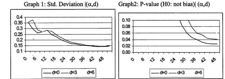
conduct a Monte Carlo experiment to estimate the efficiency of the trimmed estimator. Steps 1-3 bellow were repeated 10000 times to ca1culate the mean and the other moments of g( {1tdha) for each value ofthe grid ofthe trimming leveI (a).
1. Sample 1tj(s) セ@ セェ@ i
=
1..n2. Compute 1t(sla,d)
=
g(1tj(s),a,d).. 3. Sum 1t(sla,d) and the other moments 1t(sla,d)m m 2,3 4
Graph 1: Std. Deviation I( a,d)
r---,
0.4
0.35 0.3 0.25 0.2 0.15 0.1
セ@
",->--",- セ@
セ@
l--cFO-d=3
d=61
Graph2: P-value (HO: not bias)1 (a,d)
0.10
0.08 \ \
0.06 \
'"
.-0.04
"-....
"-0.02 '
-0.00
セ@ co ,,'l- ,,'b セ@ セセ@ セ」ッ@ セGャM
*'
1-
c1=0 -cI=3 d=61
The standard deviation of the GLS estimator for this data set is (0.129). Graphs 1 and 3 show the standard deviation of the trimmed estimator calculated as a function of (a,d) where the simple mean corresponds to the
Graph 3: Std.deviation
I
(a,d)0.38
0.33
0.28
0.23
0.18
These results indicate that: (i) a larger (u) implies greater efficiency and
greater probability of bias; (ii) a larger asymmetry coefficient (d) implies less efficiency and less probability of bias; (iii) trimming could double efficiency compared to the non-trimming case; (iv) the efficiency of the trimmed mean estimator is comparable to the efficiency of the GLS estimator although we do not lmow the volatility of the changes in the price of each product.
This exerci se shows that, for our data set, we can use the trimmed mean
to estimate the common leveI of inflation (J..L) without much efficiency loss. It
should be stressed that the GLS estimator requires the estimation of more than 300 parameters, whereas the trimmed mean involves only 2 parameters, and that the trimmed mean can be calculated using only data for each month. This means that we do not need hypothesis about the stability of the volatilities and that we can work with a data set where the number of components changes.
3.2 Estimation of the common trend
Now we turn to our fulI model (1) which alIows the common leveI (J..L)
to folIow a random walk. This is one possible way to discriminate between transitory and permanent shocks that affect alI products joint1y and that cannot be estimated using synchronic data. Core inflation is defined as
lllt=E(pt), the expected value of the common trend. This measure discards
i=1. .. N (I)
Ç,t
-(O,W)The common trend is c10se to a mean of (1tit) , so its variance should be
smaIler than the idiosyncratic shocks' variances (CJr). If we assume that it is
much smaIler and define the common trend innovation variance as a proportion of the common trend variance (W=(l/f-I)V(J.lt_Ilt-I))19, it can be
shown20 that core inflation foIlows:
ffit= fmt-l
+
(l-f)(Lp·;2r
IL/T;-2í'Z"j
== fmt-l+
(l-f) g( {1tdba.,d) (5)Where the last factor is exactly the GLS estimator of the common leveI of the price variation in month (t). Since the trimmed estimator was a good
ウオ「ウエゥエオエセ@ for GLS in the static case, we wiIl assume without test2l, that it will
be a good for each in the dynamic case too. So, we wiIl substitute the last factor in (5) by the trimmed mean estimator of the common leveI.
Given W={a.,d,f}, we have a family of core inflation measures (ffit(W)) indexed by W, each of them with a specific degree of trimness and smoothness. The maximum likelihood estimator of W is, in this case, equivalent to minimising L(E(1titlt-I)-mt-l(w)i, which is not exactly our
objective22
• The future leveI of inflation can be measured, each month, by the
mean inflation over the next h months (Xt(h))23. To emphasise the leading
character of core inflation, we propose to estimate W by minimising24
:
LS(W)= L(Xt(h)-mt(w)i (7)
As this function could have more than one extreme value, we need· a weighing function for the members of the core inflàtion family {mt(W)} to obtain unconditionated results. So, we introduce a new, and last, hypothesis
aIid assume that (xt(h) - mt(W)) foIlows a normal distribution2S
:
xt(h) - ffit(W) セ@ N(O,cr2) (7.1)
19 This is the proportional variance dynamic bayesian model of West and H!lflÍ.son (1997).
20 See the appendix.
21 We have no data for this test
22 We want to have a good local trend and not a good one period forecast. The latter approach produces core
measures with low leading capacity too.
23 X, (h) = (h + 1)
L:o
í'Z"1+; Where (1tt) is the headline IPCA indexo24 An alternative definition for (Pt(h» would be to consider the centred moving average as Bryan and Cecchetti
do. We show bellow that our definition gives better results.
Using (7.1) we can obtain one weight for each of the members of our family of core {mt("')} using the likelihood (8) to obtain this weighted function (9). We use (lO) to calculate a measure of core inflation that does not
depend on
('1').
p(",10)26 oc -0.5(Lt (Xt(h)- mt(",))2/T
r
T (8). p(V'1 O)
wVI = 1,p(V'
I
O) (9)E(m 10)
セ@
1,p(V'I
O)mt(V') = f w m () (10)t
1,
p(V'I
O)セ@
VI t V'Considering the size of the data sample and the actual characteristics of the Brazilian economy we choose h=6. Results are conditional on this value,
which is ad hoc, but, we hope, will not greatly affect the basic results.
Empirical results were done using a grid on (",) space and calculating the value of {Wt("'i), mt("'i)} for all grid points.
The mode is defined as "'i*=argmaxi p("'iIO).
Given that (xt(h)) is observed only up to h months before the last month
in the sample, model (7.1) is estimated without the last h months. In spite of
this, it should be stressed that we can calculate up-to-date values of core inflation {mt(",)} that do not depend on (h).
To isolate the effects of trimming, asymmetric trimming, and smoothing, we estimated restricted versions of the model and calculated the .'" that minimises (8) or, which is the same, that maximises (9) for each case.
To evaluate 'the effect of of future mean of inflation we estimated (",) using . the loss function LS*(.) that has the same especification ofLS(.) but (xt(h)) is
substituted by centred mean27 (Yt(h)).
The results in table 3 suggest that: (i) asymmetric trimming has a small impact on the likelihood; (ii) trimming by itself has a larger effect on the likelihood than smoothing by itself; (iii) current IPCA is a bad lead of future inflation; and (iv) we get the worst leading capacity when the core is estimated using the centred moving average of inflation.
26 Where O is the information set.
T bl 3 L·k l"h d fi a e 1 e 1 00 or speCl catlOns o ·fi . f C ore
Specification a a+d F VM*
l-only smooth 0.000 1.000 0.538 51.2
2- onlytrim 0.175 0.850 0.000 63.8
3-trim, smooth 0.125 0.850 0.538 67.0 4-trim( simm),smooth 0.481 0.519 0.692 66.3
5- IPCA O 1 O 45.3
6-trim,smooth* .15 .85 .789 60.12
* calculated with centred moving average
The unconditionated results were done using the same grid for (",) space and equations (10-12). The function w(.) given by (10) is a aproximation for the estimator distribution. The grapfs 4-6 show the parameter marginal distribution for the 3 models, only trimmed, trimmed and smoothing, and simetric trimmed and smoothing.
(10)
E(mtln) == Liw("'i)mt("'i) (11)
V(ffitln) ==LiW("'i) (mt(CPi) - E(mtln)i (12)
(0.10)
Graph 4: Only trim Model: Marginal Distribution of (dIO)
0.14 , - - - , 0.12
0.10 0.08 0.06 0.04
0.02
o .00 セNLNLNLNNLNLNNLNLNLNLNNNNLNLNLNNNNNNLNLNLNLNNN⦅LNNNNLNNNNLNNNMA@
セ@ セ@ セ@ セ@ セ@ セ@ セ@ セ@ セ@
セ@ セ@ セ@ a· セ@ セ@ セ@ セ@ セ@
0.25 , - - - ,
0.20
0.15
0.10
0.05
o . o o
+-,-,,.,.,...,.,.,.,.,.,...,.,.,,.,.,...,.,...,a.-,.-r-r-"T""T"""l
O"" 0411 012 01 CYR CYR
l'Vll
-,
002
fi
Graph 5: Complete Model: Marginal distribution
(aiO)
I 11. I II
nl IlIlIhl II
o III .... III o ... ('\I III (\') III ('\1 .(\') セ@ III lll'lll co
Nセ@ ·Ill . .0 .0 .0 .0 .0 .0
o o o o o o
(a+dIO) HセoI@
ュセKMMMセMMMMセ@
0-::;
PQKMMMMMMセMMMMMMャ@
(JJi I . _ 1
1111.-
1.111.11111
n
NMMMMMMMMMMMMMセ@
セ@
Q1+---... f . . - - - - _ _ _ l
o:B!+---... セMMMMMャ@
。bZKMMMdャャャヲiNiiiNNNMMMセ@
(D+---... J.HI.lI4b-
II
.---l
u 1 tní Ij ti
a:
(l O'la:257924691358
Graph 6: Only smooth and symmetric trim model
Marginal Distribution of(aIO) Marginal Distribution ッヲHセoI@
0.1 0.1
0.1 0.1
O. O.
0.0 0.0
0.0 0.0
0.0
I
Ih
0.0_11
0.0 11 0.0
I
1I
nl
lIi.
In
.••• II-n ..1I
o
o
n n
0.00.00.10.10.10.2).2).3).3).3).4> .4
.
0.CD.1O.2).3).l>.4UD.ED.ED.iU.ID.9- - -
-
-
-
.
-
-
- -
n セ@ " .. " ,. A " n ..,. r."' "Graphs 4-6 suggest that: (i) for alI versions of the model, (aln) and (a
+
dln) have more than one mode, which does not recommendセウエゥュ。エゥョァ@
the components of \li by maximum likelihood; (ii) the HセョI@ distribution has a
nicer behaviour than the others; (iii) mode points change with model version, indicating that parameters must be estimatedjoint1y.
Graphs 7-10 belIow show the path of each measure of core inflation28 • We notice that: (i) only trimming smoothes the path, as it should, since idiosyncratic components are discarded; (ii) the common trend between (IPCA, IP A, INCC) is somewhat volaiile; (iii) the unconditional and trim&smooth estimator are very similar, which means that the core measures calculated using either estimators are also similar.
28 Graph 8 presents a measure of core inflation that will be discussed more fully in the next section. Briefly, it
Graph 7: IPCA and one version of core inflation
Unconditioned: only smooth Unconditioned: only trim
3.0 2.0 1.5 1.0 0.5 0.0 -0.5 1111"/95 3.0 2.5 2.0
--1.5 1.0 0.5 0.0 -0.5 1111"/95 3.0 2.5 1.5 1.0 0.5 0.0 -0.51111"/96 I11I"m 1111"/98 1111"/99 1111"/95 1111"/96 1111"/97
Graph 8: IPCA and one version of core inflation
MLE: trim and smooth 3 variable model
1111"/96 3.0 2.5 2.0 1.5 1.0 0.5 0.0 3.5 3.0 , 2.5 2.0 1.5 1.0 0.5 0.0 -0.5
I11I"m 1111"/98 1111"/99 1111"/95 1111"/96 I11I"m
Graph 9: IPCA and unconditional (smooth&trim) 1111"/98
1111"/98
-0.5 -1 .0
Jan- Jul- Jan- Jul- Jan- Jul- Jan- Jul- Jan- Jul-
Jan-95 95 96 96 97 97 98 98 99 99 00
1111"/99
Graph 10: Trim&Smooth : Comparing Unconditioned and MLE versions
2.7 2.2
1.7
1.2
0.7
0.2
-0.3
,-
-
... \m a r /95 m a r /96 m a r /97 m a r /98 m a r /99
The graphs reflect the process of inflation reduction that started with the Real Plan of July 1994, as they should. Our measure of core inflation suggests that price stability could be rejected before the second half of 1997 and that the major devaluation of January 1999 had a significant impact on trend inflation. Price stability is again rejected throughout 1999. The different measures also suggest that by late 1998 the economy might be heading for deflation if policy were maintained. This helps explaining why the January
1999 devaluation did not have an even larger impact on inflation.
4. Does our measure of core inflation lead headline inflation?
Our measure of core inflation satisfies, by construction, the proprieties we mentioned above: it discards idiosyncratic and macro noises, and it is also forward-Iooking in the sense that it was constructed with an eye at tracking the h-step ahead moving average of inflation. But we do not know whether it is also forward-Iooking in the more usual sense of being a lead of headline inflation. Is it a good leading indicator? How does it compare with other leads? To answer these questions we compare the forecast capacity of our core inflation measure with a data set of non consumer prices, using a mo deI of attraction and a standard lead mo deI. For all cases we forecast inflation 6 months ahead.
common trend model29 with IPCA and two complementary indexes IP A30 and
INCC31 to serve as a benchmark; we call it the "3 variable model".
The data is the set of IP A and INCC components. They are sub-price
indexes of IGP32 that is the other main indicator of inflation in BraziP3. The
105 components of the IP A&INCC data-set represent a very diversified set of products, from agricultural inputs, to raw materiaIs, to investment products. This data set is "complementary" to IPCA in the sense that it has a higher probability of containing information not included in IPCA, since their components have other kind of products, and are measured with another
methodology34.
The attraction model (13) checks whether the deviation between current
inflation and the selected indicator (v;") is relevant to forecast the deviation
between future and cuirent inflation (1tt). When current inflation is above
(bellow) (vrn), it should tend to be decreasing (increasing), which means that
we should not reject the hypothesis that セeHoLi}N@
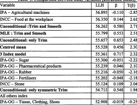
As we are forecasting h-months ahead and the model has no dynamics, residuaIs tend to be auto-correlated. So equations were estimated with an AR(1) process for errors. This model was estimated for each of our measures of core inflation, and for each component of the IP A&INCC data set and we calculated their log likelihoods (LLH). Table 4 condenses the 109 results, ordering them in descending order of (LLH) and eliminating the intermediate lines.
Table 4 shows that: (i) only two of the 105 components of the IPCA&INCC data set have a better - although not significant - forecast capacity than our selected measure of the core, but one of then gives non
sense results Hセ\oI[@ (ii) the unconditional trim&smooth and the MLE version
have almost the perfomance; (iii) the results for the presented leads are almost
29 Xit =BIlt + Dzit+ eit ,eit-N(O,L); Ilt = 1lt-1+ セL@ セMnHoLGvセI[@ Zit = cp Yit-1++Çit, Çit -N(O,v), estimated using
STAMP
30 IP A (Índice de Preços no Atacado) is wholesale price indexo
31 INCC (Índice Nacional da Construção Civil) is a price index for housing construction. 32 IGP (Índice Geral de Preços) is a measure of"general" price leveI.
33 IGP is composed of 3 sub-price indexes: IP A, the production price index of industrialised products which includes 67 elements; INCC, the price index of construction which includes 38 elements; and IPC, the consumer price indexo
the same considering the likelihood sca1e, but are significantly better than the other 1eads that have LLKe(52.9,54.7).
Table 4: Comparison between leads variables (attraction model)
Variable LLH セ@ tHセI@
IP A - Agricultural machities 56.895 -0.110 -2.85
INCC - Food at the workplace 56.350 0.144 2.61
Unconditional :Trim and Smooth 56.262 0.580 2.71
MLE : Trim and Smooth 55.799 0.553 2.51
Unconditional: only Trim 55.657 0.653 2.48
Centred mean 55.528 0.456 2.30
3 Index model 55.361 0.717 2.32
IP A-OG - Sugar 55.306 -0.051 -2.22
IP A-OG - Pharmaceutical products 55.239 0;046 2.10
IP A-OG - Rubber 55.216 -0.050 -2.16
IP A-OG - F ertilisers 55.202 -0.048 -2.18
INCC- Stone 55.124 0.109 2.04
Unconditional: only symmetric Trim 54.712 0.548 1.94
All others index
IP A-OG - Tissue, Clothing, Shoes 52.908 -0.019 -0.25
Tab1e 3 and tab1e 4 show that the best measure for core is the unconditionated and irrestricted measure. It is intersting verify if this variab1e (y) is suffcient to 1ead future inflation given each of the other variab1es of IP A&INCC data set (v;), and if these others variab1es (v;) are sufficient
given (y). Mode1 (14) exp1ain future inflation by (Vim) using a dynamic
re1ation, and our measure of core (y). Using this mode1 we can test two hypothesis: 1) Ho: (õrn=OI v;) using t-student test; and 2)Ho:(Alrn = ... =Âprn =01 y) using one F-test.
1tt =urn+ÕmYt-6 +Lkl1km1tt-k-S+Lk Akm
vセUMォ@
+Ut Ut=PkUt-l+et et ... N(O,s;) (14)Table 5: Comparison between lead variables (Iead model)
Variable P-value S T(ô) Ô
IPA-OG - Flour etc 0.02 .0303 2.56 .793
IP A-OG - Agricultural machines 0.02 .0679 2.25 .723
IP A-OG - Rubber 0.03 .0629 2.75 .883
IPA-OG - Tissue (natural) 0.04 .0403 2.22 .722
IP A -OG - F ertilisers 0.08 .0379 3.21 .989
IP A-OG - Paper etc 0.10 .0333 2.13 .699
Although we have not presented all tests, in all 105 cases, we can not exclude core inflation given the others lead variables, and its coefficient has reasonable values.
This analysis does not consider that variables can lead when used in combination. With the IP A&INCC data-set, it would be a bit hard to consider all2105 combinations ofvariables. Naturally, it is possible to construct a lead index using canonical correlation between future inflation and the data-set of components ofIPA&INCC and theirs lags. But this is another theme.
Just to make a first description of the IP A&INCC data-set, we make the canonical decomposition of the correlation matrix between all their 105 components. The first eigenvalue has about 74% of all variation suggesting that a lot of "linear" information is organised along just one direction. The 6 variables of table 5 are the sub-set of IP A&INCC which separately adds more information to the forecast of inflation. Using this sub-set we repeat the same exerci se and the first eigenvalue responds for 90% of all variation, which suggests that is not probable that analysis with more than one variable could be successful.
5. Conclusion
In this paper we build on work by other authors to develop a measure of core inflation or, more precisely, of core IPCA. We combine and extend their work in some ways. First, we define a measure of core inflation as the common trend of a multivariate dynamic model, that has, by construction, three properties. It filters idiosyncratic and transitory macro noises, and it leads the future leveI of headline inflation. Second, we show that the popular trimmed mean estimator of core inflation could be regarded as a proxy for the ideal GLS estimator for heteroskedastic data. Third, we employ an asymmetric trimmed mean estimator to take account of possible skewness of the distribution. F ourth, we obtain an unconditional measure of core inflation. This is a potentially important step given the ''unpleasant'' shape of some likelihood functions.
define a more adequate model to weight the members of the core inflation family.
Our main results are: (i) the trimmed and smoothed estimator produces the best measure of core inflation for our data set; (ii) smoothing by itself does contribute to the results but less than trimmingby itself; (iii) our measures of core inflation constructed with reference to a forward moving average of inflation are good leads of headline inflation when compared with other price indexes and with the core estimated using the centred moving average of inflation; (iv) the unconditional and MLE estimators are similar.
It is obvious that the same approach could be applied to other data sets that share the same proprieties of IPCA: a large number of components, heteroskedasticy, and one common trend.
It should be stressed that the size of our sample is a big limitation. The Real plan is a break on Brazilian price dynamics, and the sample after July 1994 has only about 60 months, with a continued trend of inflation reduction. So there is not enough price variability information to produce robust results.
We emphasise that there is no single measure of core inflation that is best for all possible uses. The measure we develop could neither be employed as· an inflation target nor be used·to discriminate supply from demand shocks. But it might be helpful as a means of checking whether a given policy is on track.
Finally, our measure of core inflation suggests that the Real Plan of July 1994 did not obtain price stability before the second half of 199735 and that the major devaluation of January 1999 had a significant impact on trend inflation.
Appendix
Let:
Xit = F'f..lt + et eit -(O,Yi) F=(1,I, .... I), i=1. .. N f..lt =f..lt-l +çt çt -(O,W) W = (l/f-l)Y(f..lt-llt)
Using the Dynamic Bayesian rnodel we have: (fltlt) - (rn.,Ct)
(fltlt-1) - (a.,Rt) where
Rt = Ct-1 +W = Ct-1/f
At = RtF Qt-l
Qt
=
F'RtF+Y == Y ifthe idiosyncratic errors are dominantCt = Rt- AtQtA' t
=
Rt - Rt F Q; 1 Qt(RtF Qt-l )'=
Rt- Rt Fy-1 F 'Rt = Rt (1- Rt y) = Ct-1/f(1- yCt-1/f)y = Fy-1F' =
Li:'
I
lirnt--+ooCt
=
f( 1-f)/y => lirnt--+ooRt = (1-f)/yrnt= at
+
At (Xit - F' at) = rnt-l + RtFy-1 (Xit - F' rnt-l)=
= rnt-l(1- RtFy-1F) + RtFy-1Xit = rnt-l(1- {(1-f)/y}y) +
HQMヲIセ@
Li
nit =r
セ@1 nOt
=frnt-l + (1-f)-
Li-
'
r
セ@Bibliography
1. Bakhshi, H., Yates, T. (1999); "To trim or not to trim?", Bank ofEngland Working Paper no. 97.
2. Blix, M. (1997); "Underlying inflation - a common trends approach", Sveriges Kiksbank Working Paper no. 23. .
3. Bryan, M. F., Cecchetti, S. G. (1993); "The CPI as a measure ofinflation",
Economic Review, Federal Reserve Bank ofCleveland, 29:4, 15-24.
4. Bryan, M. F., Cecchetti, S. G. (1994); "Measuring core inflation", in
Mankiw (1994).
5. Bryan, M. F., Cecchetti, S. G. (1999); "The monthly measurement of core inflation in Japan", Institute for Monetary and Economic Studies, Bank of Japan, Djscussion Paper 99-E-4.
6. Bryan, M. F., Cecchetti, S. G., Wiggins 11, R. L. (1997); "Efficient inflation estimation", NBER Working Paper no. 6183.
7. Cecchetti, S. G. (1997); "Measuring short-run inflation for central bankers", Economic Review, Federal Reserve Bank of Saint Louis, May/June,
143-155.
8. Cecchetti, S. G., Groshen, E. L. (2000); "Understanding inflation: implications for monetary policy", NBER Working Paper no. 7482.
9. Cogley, T. (1998); "A simple adaptive measure of core inflation", Federal Reserve Bank of San Francisco Working Papers in Applied Economic Theory no. 98-06.
19.Fase, M. M. G., Folkertsma, C. K. (1997); Bmセ。ウオイゥョセ@ inflation", De Nederlandsche Bank StaffReports no. 8.
11.Fiorencio, A. Moreira, A. (2000); "Measuring the' Stability of the Price System", forthcoming in Economic Modelling.
12.Gartner, C., Wehinger, G. D. (1998); "Core inflation in selected European Union countries", Oesterreichische Nationalbank wッセォゥョァ@ Paper no. 33.
13.Mankiw, N. G. (ed) (1994); Monetary Policy, The University of Chicago
Press.
15.Quah, D. T., Vahey, S. P. (1995); "Measuring core inflation", Bank of England Working Paper Series no. 31.
16.Roger, S. (1997); "A robust measure of core inflation in New Zealand, 1949-96", Reserve Bank ofNew Zealand Discussion Papers no. 97/7.
17.Roger, S. (1998); "Core inflation: concepts, uses and measurement", Reserve Bank ofNew Zealand Discussion Papers no. 98/9.
l8.Taillon, J. (1997); "Review of the literature on core inflation", Analytical Series no. 4, Statistics Canada.
19.Taillon, J. (1999); "Core inflation - a weighted median index", Analytical Series no. 7, Statistics Canada.
20.Valkovszky, S., Vincze, J. (2000); "Estimates of and problems with core inflation in Hungary", National Bank ofHungary Working Paper 2000/2. 21.Wynne, M. A. (1999); "Core inflation: a review of some conceptual issues", Federal Reserve Bank ofDallas Working Paper no. 99-03.
FUNDAÇÃO GETULIO VARGAS
BIBLIOTECA
ESTE VOLUME DEVE SER DEVOLVIDO À BIBLIOTECA NA ÚLTIMA DATA MARCADA
000304442
1111111111111111111111111111111111111 N.Cham. P/EPGE SPE F518m
Autor: Piorencio, Antonio.
Título: Measuring core inflation as エィセ」ッュョャPョ@ trend of