SHAHNWAZ ALAM
Department of Mechanical Engg. Integral University, Lucknow, India [email protected]
DR.M.I.KHAN
Department of Mechanical Engg. Integral University, Lucknow, India [email protected]
Abstract:
In these research paper the Design of experiment using 2-level full factorial technique has been used to conduct experiments and to develop relationships mathematical models for predicting the weld bead penetration in single wire submerged arc welding of 12 mm thick mild steel plates . The response factor, namely bead penetration, as affected by arc voltage, current, welding speed, wire feed rate and nozzle-to-plate distance have been investigated and analyzed.. The models developed have been checked for their adequacy and significance by using the analysis of variance, F-test and the t-test, respectively. Main and interaction effects of the process variables on weld bead penetration have also been presented in graphical form. The developed models could be used for the prediction of important weld bead penetration and control of the weld bead quality by selecting appropriate process parameter values. And the model-predicted penetration values have been compared with their respective experimental values.
Keywords: Submerged arc welding, welding process parameters, Weld bead penetration, Mathematical modelling and full factorial technique.
1. Introduction
Fig.-1 Experimental Set- up
Fig.2 Weld bead Penetration (P)
2. Plan of investigation.
2.1.Identification of important parameters
Review of literature and a large number of trial runs indicate that the dominant factors which are having greater influence on the responses are open circuit voltage (OCV), welding current (I) , wire feed rate (F), welding speed (S) and nozzle- to- plate distance (C) (15).
2.2.Determining the working limits of the parameters
Extensive trial runs have been carried out to find out the feasible working limits of submerged arc welding parameters on mild steel. Different combinations of open circuit voltage (OCV), welding current (I) wire feed rate (F), welding speed (S) and nozzle- to- plate distance (C) were used to observe the effect on desired response. The weld zones were inspected with visual inspection to identify the working limits of the welding parameters.
2.3.Developing the experimental design matrix
The feasible limits of the parameters were selected in such a way that the welds obtained were free from surface defects. A two level full factorial design of (25-1 = 32) thirty two experimental runs, which is a standard statistical tool to investigate the effects of number of parameters on the required response, was selected for determining the effect of five independent direct welding parameters. This technique reduces the costs and provides the required information about the main and interaction effects. The commonly employed method of varying one parameter at a time, though popular, does not give any information about interaction among parameters. Table -1 presents the working range of factors considered. For the convenience of the recording and processing the experimental data the upper and lower levels of the factors are coded as -1 and +1 respectively.
2.4. Conducting the experiments as per designed matrix
welded plates. These specimens were cleaned, ground, polished and etched with 10% nital (90% alcohol + 10% of nitric acid). All specimens of first set were macro etched to reveal the bead profile and some specimens of second set were micro etched to reveal the microstructures. Weld bead profiles were traced by using an optical profile projector/Image at 20X magnification and the magnified view was drawn on the transparencies for further analysis. Measurements were made for bead penetration (P). The observed values of the responses are given in table.3.
2.4.1. Base Metal
Test specimens were prepared from 12 mm thickness Mild steel plate, 295x145x12mm size with a composition of (C-0.102%,S-0.179%,Mn-0.466%,S-0.0705%,Cr-0.036%,Ni-0.022%).
2.4.2. Flux used
The study was carried out by using the available agglomerated flux, automelt GR-4 with a composition of (C-0.08%, Mn-1.00%, Sn-0.25%).
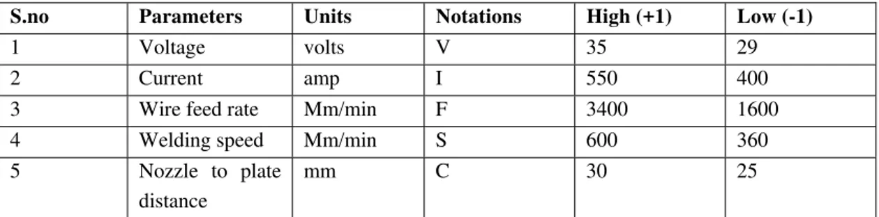
Table1. Important process control variables
S.no Parameters Units Notations High (+1) Low (-1)
1 Voltage volts V 35 29
2 Current amp I 550 400
3 Wire feed rate Mm/min F 3400 1600
4 Welding speed Mm/min S 600 360
5 Nozzle to plate distance
mm C 30 25
2.5. Selection of the useful limits of the welding parameter:
Trial runs were carried out by varying one of the process parameters whilst keeping the rest of them at constant values. The working range was decided upon by inspecting the bead for smooth appearance and the absences of any visible defects. The upper limit of a factor was coded as +1 and lower limit as -1. The selected process parameters with their limits, units and notation are given in Table.1 above.
2.6. Developing the design matrix
The designed matrix is given below the level (or signs) for the parameter C (nozzle to plate distance) are derived by the relation C=V*I*F*S
Table 2. Design matrix
Weld. no V
volts
I amp
F mm/min
S mm/m
C* mm
Treatment combination+ve
10 -1 +1 -1 +1 +1 ISC 11 -1 +1 -1 -1 -1 I 12 -1 +1 -1 +1 +1 ISC 13 -1 +1 +1 -1 +1 IFC 14 -1 +1 +1 +1 -1 IFS 15 -1 +1 +1 -1 +1 IFC 16 -1 +1 +1 +1 +1 VIFSC 17 +1 -1 -1 -1 -1 V 18 +1 -1 -1 +1 +1 VSC 19 +1 -1 -1 -1 -1 V 20 +1 -1 -1 +1 +1 VSC 21 +1 -1 +1 -1 +1 VFC 22 +1 -1 +1 +1 -1 VFS 23 +1 -1 +1 -1 +1 VFC 24 +1 -1 +1 +1 -1 VFS 25 +1 +1 -1 -1 +1 VIC 26 +1 +1 -1 +1 -1 VIS 27 +1 +1 -1 -1 +1 VIC 28 +1 +1 -1 +1 -1 VIS 29 +1 +1 +1 -1 -1 VIF 30 +1 +1 +1 +1 +1 VIFSC 31 +1 +1 +1 -1 -1 VIF 32 +1 +1 +1 +1 +1 VIFSC The numbers in the first column indicate the number of trial run
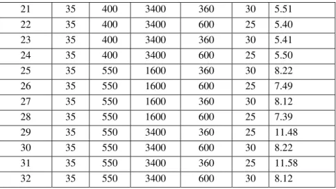
Table- 3. The observed values of the responces.
Weld. No V volt I Amp F mm/min S mm/min C mm Penetration (P)mm
1 29 400 1600 360 30 2.80
2 29 400 1600 600 25 3.16
3 29 400 1600 360 30 2.70
4 29 400 1600 600 25 3.06
5 29 400 3400 360 25 5.11
6 29 400 3400 600 30 2.80
7 29 400 3400 360 25 5.01
8 29 400 3400 600 30 2.70
9 29 550 1600 360 25 4.69
10 29 550 1600 600 30 4.52
11 29 550 1600 360 25 4.59
12 29 550 1600 600 30 4.42
13 29 550 3400 360 30 4.62
14 29 550 3400 600 25 4.61
15 29 550 3400 360 30 4.52
16 29 550 3400 600 30 4.52
17 35 400 1600 360 25 5.50
18 35 400 1600 600 30 3.66
19 35 400 1600 360 25 5.50
29 35 550 3400 360 25 11.48
30 35 550 3400 600 30 8.22
31 35 550 3400 360 25 11.58
32 35 550 3400 600 30 8.12
2.7. Development of mathematical models
Mathematical models can now be developed for the SAW process to predict weld bead penetration and to establish the interrelationship between welding process parameters to weld bead penetration. The experimental data were used to develop linear models, and analysis of the models was carried out through ANOVA and Minitab software was used for this purpose.
The general response function representing any of the weld-bead dimensions can be Expressed as Y. = ƒ (V, I, F, S, C)
Where, Y= Weld bead response, V= Open Arc voltage, I= Current=Wire feed rate, S= Welding speed, and C= Nozzle-to-plate distance.
The effect caused by change in five main factors and their first order interaction can be expressed as the relationship selected being a first order linear equation
Y=b0+b*V+b2*I+b3*F+b4*S+b5*C+b12*VI+b13*VF+b14*VS++b15*VC+b23*IF+b24*IS+b25*IC+b34*FS +b35*FC+b45*SC
Where Y represents any of the weld bead dimensions , b0 is constant and b1,b2,b3,b4,b5,b11 , b12,b13,b14,b15,b23,b24,b25,b34,b35,b45 are co-efficient of the model.
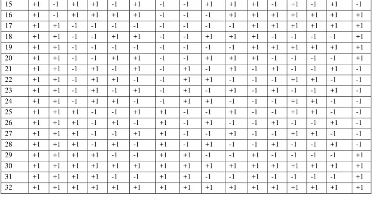
Signs for calculating effects of parameters and their interactions. The signs for the interaction were obtained by multiplying the corresponding signs of the involved factors (Table.4)
Table 4. The signs for main and interaction effects.
Trial no
X0 V I F S C VI VF VS VC IF IS IC FS FC SC
15 +1 -1 +1 +1 -1 +1 -1 -1 +1 +1 +1 -1 +1 -1 +1 -1 16 +1 -1 +1 +1 +1 +1 -1 -1 -1 +1 +1 +1 +1 +1 +1 +1 17 +1 +1 -1 -1 -1 -1 -1 -1 -1 -1 +1 +1 +1 +1 +1 +1 18 +1 +1 -1 -1 +1 +1 -1 -1 +1 +1 +1 -1 -1 -1 -1 +1 19 +1 +1 -1 -1 -1 -1 -1 -1 -1 -1 +1 +1 +1 +1 +1 +1 20 +1 +1 -1 -1 +1 +1 -1 -1 +1 +1 +1 -1 -1 -1 -1 +1 21 +1 +1 -1 +1 -1 +1 -1 +1 -1 +1 -1 +1 -1 -1 +1 -1 22 +1 +1 -1 +1 +1 -1 -1 +1 +1 -1 -1 -1 +1 +1 -1 -1 23 +1 +1 -1 +1 -1 +1 -1 +1 -1 +1 -1 +1 -1 -1 +1 -1 24 +1 +1 -1 +1 +1 -1 -1 +1 +1 -1 -1 -1 +1 +1 -1 -1 25 +1 +1 +1 -1 -1 +1 +1 -1 -1 +1 -1 -1 +1 +1 -1 -1 26 +1 +1 +1 -1 +1 -1 +1 -1 +1 -1 -1 +1 -1 -1 +1 -1 27 +1 +1 +1 -1 -1 +1 +1 -1 -1 +1 -1 -1 +1 +1 -1 -1 28 +1 +1 +1 -1 +1 -1 +1 -1 +1 -1 -1 +1 -1 -1 +1 -1 29 +1 +1 +1 +1 -1 -1 +1 +1 -1 -1 +1 -1 -1 -1 -1 +1 30 +1 +1 +1 +1 +1 +1 +1 +1 +1 +1 +1 +1 +1 +1 +1 +1 31 +1 +1 +1 +1 -1 -1 +1 +1 -1 -1 +1 -1 -1 -1 -1 +1 32 +1 +1 +1 +1 +1 +1 +1 +1 +1 +1 +1 +1 +1 +1 +1 +1
Table 5. Coefficients of the models
Serial no Coefficients Bj Penetration
(P)
1 B0 5.50251
2 B1 1.41374
3 B2 1.29126
4 B3 0.50756
5 B4 -0.49119
6 B5 -0.42275
7 B12 0.61999
8 B13 0.22869
9 B14 -0.25756
10 B15 -0.13480
11 B23 0.03881
12 B24 -0.00994
13 B25 0.14600
14 B34 -0.22114
15 B35 -0.24520
16 B45 0.26605
2.8. Evaluation of the co-efficient of the model
The values of the coefficients of the linear equation were calculated by the regression method. The Minitab and SPSS software package were used to calculate the values of these coefficients for different responses. All the coefficients were tested for their significance at 95% confidence level applying student’s t-test.
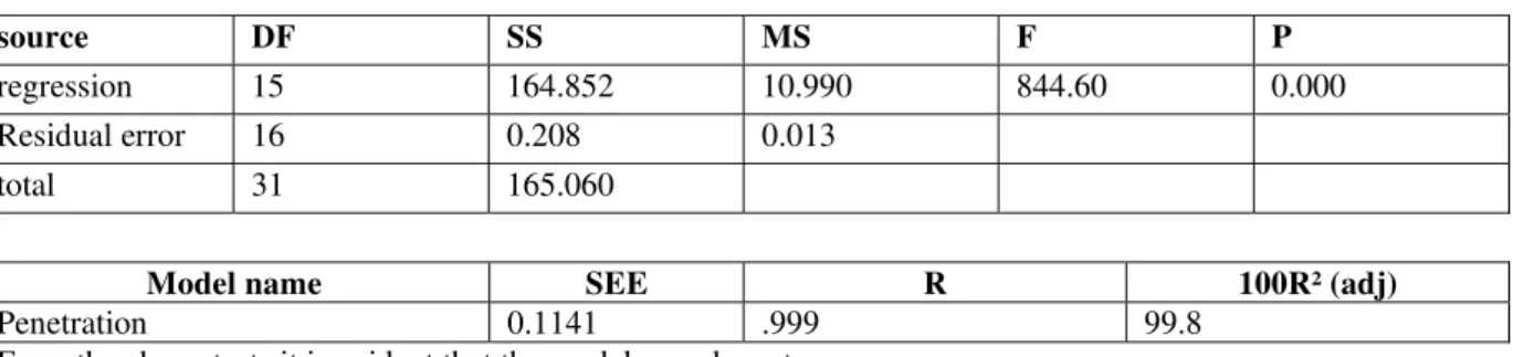
2.9. Response
regression 15 164.852 10.990 844.60 0.000
Residual error 16 0.208 0.013
total 31 165.060
Model name SEE R 100R² (adj)
Penetration 0.1141 .999 99.8
From the above tests it is evident that the model are adequate. 2.11. T- Test for significance of regression coefficients
The determination of co-efficient (R2) indicates the goodness of the fit for the model. In the case of penetration, the value of the determination co-efficient (R2 = 0.999) indicates the high level of significance. Scatter diagram between actual and predicted values of reinforcement height has been presented in Fig.3. It can be observed that there is a good correlation between the actual and predicted values which further supports the validity of developed model.
2.12. Predicted response: The final mathematical model
Penetration was expressed as a linear function of the input process Parameters (in coded form) as follow as:
Y=5.50-1.41*V-1.29*I+0.508*F-0.491*S-0.423*C+0.620*VI+0.229*VF-0.258*VS-0.135*VC+0.146*IC-0.221*FS-0.245*FC+0.266*SC
Fig.3 Plot of actual vs. predicted response of penetration.
3. Results and discussion:
The predicted influences of the welding parameters on the weld bead penetration within the range of investigation are shown in Fig.4.and the interaction effects between variables are shown in Fig.5.1 to Fig.5.5.
3.1.Direct effect or main effect of process parameters on penetration:
Fig.4 Main effect plot for penetration.
3.2. Major interaction effect of process parameters on penetration:
It is seen from Fig.5.1 that at high voltage value the penetration rapidly increases with increase in current, however at low voltage value penetration increase at very slow rate with increase in current. Fig.-5.2 shows that as the high voltage value the penetration increases with increase in wire feed rate, however at lower voltage value the penetration increases at very slow rate with increase in wire feed rate. It evident from Fig.-5.3 that the penetration decreases with increase in welding speed at high voltage value and penetration is very less at low voltage value ,it is due to that at high welding speed, the heat input per unit length decreases and so penetration will also decreases. Fig.-5.4 show that as the high wire feed rate, the penetration decreases rapidly with increases in nozzle to plate distance, however at low wire feed rate the penetration decrease in significantly with increase in nozzle to plate distance, It is due to resistance heating of the wire before the formation of an arc which results in higher metal deposition rate owing to higher heat input. Fig.-5.5 show that as the low welding speed , the penetration decreases rapidly with increases in nozzle to plate distance, however at high welding speed the penetration decreases insignificantly with increase in nozzle to plate distance.
Fig.5.1
Fig.5.2
Fig.5.3
Fig.5.4
Fig.5.5
4. Conclusions
[4] D. Kim, M. Kang, S. Rhee, Determination Of Optimal Welding Conditions With A Controlled Random Search Procedure, Welding Journal 8 (2005) 125-130.
[5] J. Raveendra, R.S. Parmar, Mathematical Models To Predict Weld Bead Geometry For Flux Cored Arc Welding, Metal Construction 19/2 (1987) 31-35.
[6] L.J. Yang, R.S. Chandel, M.J. Bibby, The Effects Of Process Variables On The Weld Deposit Area Of Submerged Arc Welds, Welding Journal 72/1 (1993) 11-18.
[7] R.S. Chandel, H.P. Seow, F.L. Cheong, “Effect Of Increasing Deposition Rate On The Bead Geometry Of Submerged Arc Welds” ,Journal of Materials Processing Technology.72 (1997)124 – 128.
[8] S. Datta, M. Sundar, A. Bandyopadhyay, P.K. Pal, S.C. Roy, G. Nandi, Statistical Modeling For Predicting Bead Volume Of Submerged Arc Butt Welds, Australasian Welding Journal 51/2 (2006) 39-47.
[9] Gupta and Parmar ,Fractional Factorial Technique To Predict Dimensions Of The Weld Bead In Automatic Submerged Arc Welding , J Inst Engr (India), 70 (1986) 67-71