www.atmos-chem-phys.net/14/3231/2014/ doi:10.5194/acp-14-3231-2014
© Author(s) 2014. CC Attribution 3.0 License.
Atmospheric
Chemistry
and Physics
Arctic stratospheric dehydration – Part 2: Microphysical modeling
I. Engel1,*, B. P. Luo1, S. M. Khaykin2,3, F. G. Wienhold1, H. Vömel4, R. Kivi5, C. R. Hoyle6,7, J.-U. Grooß8, M. C. Pitts9, and T. Peter1
1Institute for Atmospheric and Climate Science, ETH Zurich, Zurich, Switzerland 2Central Aerological Observatory, Dolgoprudny, Moscow Region, Russia
3LATMOS-IPSL, Université Versailles St. Quentin, CNRS/INSU, Guyancourt, France
4Deutscher Wetterdienst, Meteorological Observatory Lindenberg – Richard Aßmann Observatory, Lindenberg, Germany 5Finnish Meteorological Institute, Arctic Research, Sodankylä, Finland
6Laboratory of Atmospheric Chemistry, Paul Scherrer Institute, Villigen, Switzerland
7Swiss Federal Institute for Forest Snow and Landscape Research (WSL) – Institute for Snow and Avalanche Research (SLF),
Davos, Switzerland
8Institut für Energie- und Klimaforschung – Stratosphäre (IEK-7), Forschungszentrum Jülich, Jülich, Germany 9NASA Langley Research Center, Hampton, Virginia, USA
*now at: Institut für Energie- und Klimaforschung – Stratosphäre (IEK-7), Forschungszentrum Jülich, Jülich, Germany
Correspondence to: I. Engel ([email protected])
Received: 13 August 2013 – Published in Atmos. Chem. Phys. Discuss.: 18 October 2013 Revised: 14 February 2014 – Accepted: 18 February 2014 – Published: 2 April 2014
Abstract. Large areas of synoptic-scale ice PSCs (po-lar stratospheric clouds) distinguished the Arctic winter 2009/2010 from other years and revealed unprecedented ev-idence of water redistribution in the stratosphere. A unique snapshot of water vapor repartitioning into ice particles was obtained under extremely cold Arctic conditions with tem-peratures around 183 K. Balloon-borne, aircraft and satellite-based measurements suggest that synoptic-scale ice PSCs and concurrent reductions and enhancements in water va-por are tightly linked with the observed de- and rehydra-tion signatures, respectively. In a companion paper (Part 1), water vapor and aerosol backscatter measurements from the RECONCILE (Reconciliation of essential process parame-ters for an enhanced predictability of Arctic stratospheric ozone loss and its climate interactions) and LAPBIAT-II (La-pland Atmosphere–Biosphere Facility) field campaigns have been analyzed in detail. This paper uses a column version of the Zurich Optical and Microphysical box Model (ZOMM) including newly developed NAT (nitric acid trihydrate) and ice nucleation parameterizations. Particle sedimentation is calculated in order to simulate the vertical redistribution of chemical species such as water and nitric acid. Despite lim-itations given by wind shear and uncertainties in the ini-tial water vapor profile, the column modeling unequivocally
shows that (1) accounting for small-scale temperature fluc-tuations along the trajectories is essential in order to reach agreement between simulated optical cloud properties and observations, and (2) the use of recently developed heteroge-neous ice nucleation parameterizations allows the reproduc-tion of the observed signatures of de- and rehydrareproduc-tion. Con-versely, the vertical redistribution of water measured can-not be explained in terms of homogeneous nucleation of ice clouds, whose particle radii remain too small to cause signif-icant dehydration.
1 Introduction
Polar stratospheric clouds (PSCs) may form in the lower stratosphere above the winter poles at sufficiently low peratures. Ice PSCs require the coldest conditions, with tem-peratures about 3 K below the frost point (Tfrost) to nucleate
than in the Antarctic stratosphere and therefore the forma-tion of ice PSCs and the occurrence of dehydraforma-tion events is relatively infrequent. Some observations of ice PSCs and water vapor depleted regions from the coldest Arctic win-ters are published in the literature (e.g., Fahey et al., 1990; Vömel et al., 1997; Jimenez et al., 2006; Maturilli and Dörn-brack, 2006). However, these studies did not observe such a clear case of vertical redistribution of water vapor as that presented here, which occurred above Sodankylä during the Arctic winter 2009/2010.
This paper presents vertical profiles of water vapor and aerosol backscatter obtained within the framework of the LAPBIAT-II (Lapland Atmosphere–Biosphere Facility) bal-loon campaign in January 2010 from Sodankylä, Finland, which was closely related to the RECONCILE (Reconcili-ation of essential process parameters for an enhanced pre-dictability of Arctic stratospheric ozone loss and its climate interactions) project and its activities in the same Arctic win-ter (von Hobe et al., 2013). Whereas the majority of Arc-tic PSC studies describe wave ice cloud observations above Scandinavia (e.g., Carslaw et al., 1998b; Fueglistaler et al., 2003), we present model simulations based on observations of rare synoptic-scale ice clouds. A week-long period (15 to 21 January 2010) of unusually cold temperatures at strato-spheric levels led to the formation of synoptic-scale ice PSCs (Pitts et al., 2011). Balloon-borne measurements of parti-cle backscatter and water vapor on 17 January captured an ice PSC and the concurrent uptake of water from the gas phase in fine detail, providing a high-resolution snapshot of the process of ice PSC formation. A vertical redistribution of water inside the vortex, which was tracked remotely and could be quantified again by in situ measurements some five days later, was observed in the Arctic stratosphere for the first time. A companion paper (Khaykin et al., 2013) presents the series of in situ observations in January 2010 above So-dankylä, which coincide with vortex-wide satellite measure-ments. This study connects two individual balloon soundings by trajectories and simulates the formation, growth and sed-imentation of the ice particles.
Very recently, the commonly accepted theories describing the formation mechanisms of PSCs have been revised. Ho-mogeneous freezing of supercooled ternary solution (STS) droplets is the generally accepted formation pathway for ice PSCs, requiring a supercooling ofT .Tfrost−3 K (e.g.,
Koop et al., 1995, 2000). The importance of heterogeneous ice nucleation for PSC formation was shown by Engel et al. (2013), together with a study by Hoyle et al. (2013), which reconciled the current theory of nitric acid trihydrate (NAT) nucleation with observed PSC characteristics.
This study uses a column version of the Zurich Optical and Microphysical box Model (ZOMM) including the newly de-veloped NAT and ice nucleation parameterizations. Similar to the one-dimensional version of ZOMM, the new column version allows the simulation of the nucleation and growth of PSC particles and the associated reduction in water vapor.
Additionally, because sedimentation is included, the column version can be used to follow trajectories over longer periods of time and thus allows the simulation of the observed de-hydration of the Arctic stratosphere. Caveats of this method will be discussed in Sect. 2.4.1.
In this study, we examine the effect of different nucleation mechanisms, in particular homogeneous vs. heterogeneous ice formation, as well as temperature fluctuations, on PSC properties. The overall goal of this work is to compare the modeled microphysics with the observations and thus test the newly proposed heterogeneous ice nucleation parameteriza-tions. We show that in order to successfully reproduce the observed dehydration and rehydration, heterogeneous nucle-ation and temperature fluctunucle-ations must be accounted for in the model.
2 Methods
The following section provides a short overview of the mea-surement techniques used to obtain the data for this study. Furthermore, the trajectory calculation tool and the micro-physical column model are characterized. A more compre-hensive description of the different instruments is given in the companion paper by Khaykin et al. (2013).
2.1 Backscatter measurements
Backscatter measurements from balloon- and spaceborne in-struments are utilized in this work. The Compact Optical Backscatter Detector (COBALD) is a backscatter sonde, en-gineered at ETH Zurich, complementing operational weather balloon payloads. The sonde is a follow-up development of the backscatter sonde designed by Rosen and Kjome (1991). Two LEDs emitting at wavelengths of 455 nm and 870 nm are aligned in parallel and located to the left and right of a silicon detector. The light scattered back by air molecules, aerosols and cloud particles is recorded with a typical frequency of 1 Hz. The data analysis follows Rosen and Kjome (1991) to separate the individual contributions from molecules and aerosols to the measured backscatter signal. The molec-ular air number density is derived from temperature and pressure recorded simultaneously by the radiosonde hosting COBALD. A direct indicator for the presence of aerosols is the backscatter ratio (BSR): it is defined as the ratio of the total (aerosol and molecular) to the molecular backscattered light intensity (at∼180◦back to the detector). Accordingly,
the aerosol backscatter ratio is equal to BSR−1. COBALD has already been applied in several different field studies, for example, measuring the volcanic aerosol plume after the eruption of the Eyjafjallajökull (Bukowiecki et al., 2011) and cirrus clouds (Brabec et al., 2012; Cirisan et al., 2013).
obtained by the Cloud-Aerosol Lidar with Orthogonal Po-larization (CALIOP). The satellite completes 14.5 orbits per day and has a near-global coverage, ranging from 82◦N to
82◦S (Winker et al., 2007). CALIPSO’s orbit inclination
and its associated extensive polar coverage make the satel-lite an ideal platform for PSC observations. For this purpose, Pitts et al. (2007, 2009) introduced a detection algorithm to identify and further classify PSCs. Their composition clas-sification is based on BSR at a wavelength of 532 nm and aerosol depolarization (δaerosol) obtained from the CALIOP
Level 1B data product. The data is averaged to a uniform grid with a horizontal resolution of 5 km and a vertical res-olution of 180 m. Pitts et al. (2011) distinguish six different PSC composition classes with varying number densities of liquid, NAT and ice particles.
2.2 Water vapor and nitric acid measurements
Balloon-borne water vapor measurements are obtained by two different techniques. The Fluorescence Lyman-Alpha Stratospheric Hygrometer for Balloons (FLASH-B) is a Rus-sian water vapor instrument developed at the Central Aero-logical Observatory (Yushkov et al., 1998). The fluorescence method uses the photodissociation of H2O molecules
ex-posed to Lyman-alpha radiation followed by the measure-ment of the fluorescence of the resulting excited OH radi-cals (Kley and Stone, 1978). The intensity of the fluorescent light sensed by the photomultiplier is directly proportional to the water vapor mixing ratio under stratospheric conditions (10 hPa to 150 hPa). The second instrument used within this study is the Cryogenic Frost point Hygrometer (CFH), which was developed at the University of Colorado (Vömel et al., 2007a). The instrument’s principle is based on a chilled mir-ror. The temperature of the mirror can be regulated such that a thin but constant layer of frozen condensate covers the sur-face. The thickness of the frozen layer is controlled by a pho-todiode connected to an LED. The phopho-todiode measures vari-ations of the reflected light caused by changes in the thick-ness of the condensate, which feeds back into the regulation of the mirror temperature. Under these conditions,Tfrost of
the surrounding air is equal to the mirror temperature. The re-ported overall uncertainty, which includes accuracy and pre-cision, for both instruments in the middle stratosphere is less than 10 % (Vömel et al., 2007b).
Water vapor and nitric acid were measured using the Mi-crowave Limb Sounder (MLS) aboard the Aura satellite. MLS provides atmospheric profiles of temperature and com-position (including H2O and HNO3) via passive
measure-ment of microwave thermal emission from the limb of the Earth’s atmosphere (Waters et al., 2006). Vertical scans are performed every 25 s, corresponding to a distance of 165 km along the orbit track. Vertical and horizontal along-track res-olutions are 3.1 km to 3.5 km and 180 km to 290 km, respec-tively, for H2O, and 3.5 km to 5.5 km and 400 km to 550 km
for HNO3. Aura flies in formation with CALIPSO in the
A-train satellite constellation and CALIOP and MLS measure-ment tracks are closely aligned. The spatial and temporal dif-ferences are less than 10 km and 30 s after a repositioning of the Aura satellite in April 2008 (Lambert et al., 2012). MLS water vapor profiles presented in this study are inter-polated to the CALIOP PSC grid using a weighted average of the two nearest MLS profiles (Pitts et al., 2013). Typical single-profile precisions of the MLS version 3.3 measure-ments (Livesey et al., 2011) are 4 % to 15 % for H2O (Read
et al., 2007; Lambert et al., 2007) and 0.7 ppbv for HNO3
(Santee et al., 2007).
2.3 Trajectory calculations
The trajectories used within this study are calculated from six-hourly wind and temperature fields of the ERA-Interim reanalysis produced by the European Centre for Medium-Range Weather Forecasts (ECMWF) (Dee et al., 2011), with a horizontal resolution of 1◦
×1◦. We used the trajectory
module of the Chemical Lagrangian Model of the Strato-sphere (CLaMS) (McKenna et al., 2002) to calculate trajec-tories for the microphysical study. Vertical velocities are de-rived from ERA-Interim total diabatic heating rates (Ploeger et al., 2010). Starting at 19:47 UTC on 17 January 2010, a balloon sounding was performed from Sodankylä (here-after referred to as S1). Individual balloon positions along its pathway at pressure levels<100 hPa served as start points
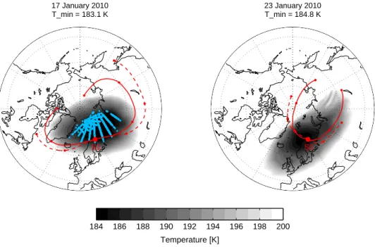
for the first set of trajectory calculations. With a vertical dis-tance of 100 m between two trajectories, two-day backward and three-day forward trajectories with time steps of 15 min were computed. A second sonde was launched on 23 Jan-uary 2010 at 17:30 UTC (hereafter referred to as S2), for which three-day backward and two-day forward trajectories in the same altitude range as for the first sounding have been calculated. Figure 1 illustrates the pathways of two exem-plary trajectories for each sounding within the Arctic vortex. It is apparent that Sodankylä was located in the cold pool with temperatures as low as 183 K as measured by the son-des, while upstream the air was more than 10 K warmer. On 17 January Sodankylä was at the edge of a larger area of synoptic-scale ice clouds seen by CALIOP.
Pressure and temperature from the joined backward and forward trajectories constitute the meteorological input for the microphysical model. Additionally, information about to-tal water and nitric acid mixing ratios is needed at the up-stream end of the trajectories. For S1, HNO3 values were
taken from MLS, averaged for the corresponding day over cloud-free areas within the vortex and vertically interpolated to the starting pressure of the trajectories. Vertically resolved climatological mean values for January were used as H2O
in-put. The H2O profile is calculated from ice-cloud-free
S1 17 January 2010 T_min = 183.1 K
S2 23 January 2010 T_min = 184.8 K
Temperature [K]
184 186 188 190 192 194 196 198 200
Fig. 1. Polar maps with ERA-Interim temperatures at 30 hPa (grayscale) on 17 January 2010 (left) and 23 January 2010 (right). Red curves:
CLaMS trajectories starting on these day above Sodankylä at 520 K (solid) and 440 K (dashed) potential temperature. Trajectories are two days backward and three days forward in time for 17 January 2010 (S1) and three days backward and two days forward in time for 23 January 2010 (S2). Red dots: 24 h time periods along the trajectories. Cyan points: ice clouds observed by CALIOP on 17 and 18 January 2010 between 16 km and 30 km altitude. No ice clouds were observed by CALIOP on 23 January 2010.
were initialized with the H2O and HNO3 profiles from S1
att=21 days. Even though a horizontal displacement exists
between the individual trajectory end and start points of S1 and S2, respectively, the approach is justified given the tem-perature distribution on vortex scale: at points where trajec-tories are matched, temperatures were above 200 K, ensuring cloud-free air and thus no change in the H2O distribution.
Trajectory temperatures were corrected according to Fig. 2, showing temperature deviations between ERA-Interim reanalysis data and measurements, taken by the Vaisala RS-92 on S1. The total measurement uncertainty for the temperature sensor is 0.5 K with an accuracy of 0.3 K between 100 hPa and 20 hPa as specified by Vaisala. Be-tween 32 hPa and 25 hPa, ERA-Interim temperatures were more than 1.5 K too warm compared to the measured tem-peratures. The temperature deviation coincides with the ob-served ice cloud, which cannot be reproduced using origi-nal ERA-Interim temperatures, as shown below. Assuming that the temperature difference is caused by a local cold pool not resolved in the ERA-Interim data, temperatures along the trajectories were changed only within a short time window around the observation. The amplitude of the applied temper-ature correction is assumed to decrease (using a sine curve) with increasing time from the observation (vertical red line in Fig. 2c) and equals zero 12 h before and after the obser-vation. Figure 2c illustrates an exemplary trajectory without (black dashed line) and with (red solid line) applied tempera-ture correction. In the absence of better knowledge, the
max-imum amplitude is assumed to occur at the sonde flight path and is assumed to be altitude dependent as shown in Fig. 2b (red line).
2.3.1 Small-scale temperature fluctuations
180 185 190 195 200 20
30
50
80
Temperature [K]
Pressure [hPa]
(a)
−1.5 0 1.5 580
520
460
400
∆T [K] (b)
Approx. potential temperature [K]
17.25 17.5 17.75 18 18.25 18.5
182 184 186 188 190 192
Day of the year
Temperature [K]
(c)
Fig. 2. (a) Black solid line: temperatures measured with the Vaisala
RS-92 radiosonde launched from Sodankylä on 17 January 2010 (S1). Black dashed line: ERA-Interim reanalysis temperatures in-terpolated in time and space to the position of the drifting balloon. Blue dashed line: frost point temperature calculated from the cli-matological mean water vapor profile. (b) Difference between mea-surement and ERA-Interim as shown in (a). Red line: temperature correction applied to the trajectories between 32 hPa and 25 hPa.
(c) Black dashed line: exemplary ERA-Interim trajectory at S1 for
29 hPa. Blue dashed line: frost point temperature calculated from the climatological mean water vapor profile. Red solid line: ERA-Interim trajectory with temperature correction. Black solid line: ERA-Interim trajectory with temperature correction and superim-posed small-scale fluctuations. See text for details.
fluctuations. Only wavelengths <400 km were considered,
which are not resolved in the ERA-Interim wind fields used in our trajectory calculations. The temperature fluctuations were superimposed onto the synoptic-scale trajectories with random frequencies and a temporal resolution of 1 s as seen in Fig. 2c (black solid line). Typical peak-to-peak fluctua-tions are about 1 K. Following Gary (2006), the Gaussian’s “full-width at half-maximum” of a temperature differences histogram is 1.2 K.
2.4 Microphysical column model
The new column version of ZOMM with implemented het-erogeneous ice and NAT nucleation rates is used to simulate the formation, evolution and sedimentation of ice particles along trajectories. The underlying model, utilized for PSC simulations, has been described by Meilinger et al. (1995)
and Luo et al. (2003b) and recently extended by Hoyle et al. (2013) and Engel et al. (2013). The following section pro-vides an overview of the modifications made to ZOMM for the purposes of this study.
ZOMM can be initialized with a lognormally distributed population of supercooled binary solution (SBS) droplets, described by a mode radius, number density and distribution width, typical for winter polar stratospheric background con-ditions (Dye et al., 1992). Driven by temperature and pres-sure data along trajectories, the uptake and release of nitric acid and water in ternary solution droplets is determined. The total amounts of H2O, H2SO4 and HNO3contained in the
air parcel are set at the beginning of the trajectory. A mix-ing of air parcels is not possible and therefore the sum of the gas and particle phase remains constant unless sedimentation takes place. The mass of sedimenting NAT and ice particles is conserved as described below. Distributed across 26 radius bins when the model is initialized, droplets are henceforward allowed to grow and shrink in a fully kinetic treatment and without being restricted to the initial lognormal shape of the distribution (Meilinger et al., 1995). The formation of solid particles results in an initiation of additional size bins. Ho-mogeneous ice nucleation in STS droplets is calculated as is heterogeneous nucleation of ice on foreign nuclei and NAT surfaces. NAT nucleation is implemented as deposition nu-cleation on ice particles and as immersion freezing on for-eign nuclei. Whereas homogeneous ice nucleation, follow-ing Koop et al. (2000), and NAT nucleation on uncoated ice surfaces, described in detail in Luo et al. (2003b), have been accepted pathways of PSC formation for many years now, the possibility of PSC formation via heterogeneous ice and NAT nucleation on foreign nuclei (e.g., Tolbert and Toon, 2001; Drdla et al., 2002; Voigt et al., 2005) had until previ-ously only a narrow observational data basis so that definitive conclusions about nucleation rates were not possible; further-more, any clear support from laboratory measurements was lacking (see detailed discussion by Peter and Grooß, 2012). The observational impasse has been overcome recently by the wealth of CALIOP PSC observations on NAT and ice PSCs obtained in the winter 2009/2010 (Pitts et al., 2011), which unmistakably reveals that both particle types must have nucleated heterogeneously. A heterogeneous nucleation mechanism, occurring on preexisting particle surfaces, for example, on meteoritic particles, has been developed to ex-plain CALIOP PSC observations over the Arctic in Decem-ber 2009 and January 2010. The parameterizations, based on active site theory (Marcolli et al., 2007), for NAT and ice are given in Hoyle et al. (2013) and Engel et al. (2013), respec-tively. These studies used ZOMM in a pure box model con-figuration, and limitations caused by neglecting sedimenta-tion of NAT and ice particles in the winter polar stratosphere were already pointed out by these authors.
2003a; Brabec et al., 2012; Cirisan et al., 2013). Sedimenta-tion of ice and NAT particles is realized by allowing particles to sediment within the advected column from one box to the next lower one. For the present study the column consists of a stack of 100 m thick boxes and the timestep for sedi-mentation is 15 min. Once ice or NAT particles grow to sizes large enough to sediment, the appropriate fraction of parti-cles is removed from its current box and, according to its size-dependent sedimentation speed, injected into the next lower box. Sedimented particles are distributed equally over the entire box. Number and mass of the particles are con-served.
The optical properties of the simulated PSCs are calcu-lated using Mie and T-Matrix scattering codes (Mishchenko et al., 2010) to compute optical parameters for size-resolved number densities of STS, NAT and ice. The refractive in-dex for STS is assumed to be 1.44 (Krieger et al., 2000). For NAT, a refractive index of 1.48 was chosen, as used in several earlier studies (e.g., Carslaw et al., 1998a; Luo et al., 2003b; Fueglistaler et al., 2003). The refractive index for wa-ter ice is 1.31 (Warren, 1984). Following Engel et al. (2013), both crystals are treated as prolate spheroids with aspect ra-tios of 0.9 (diameter-to-length ratio). T-Matrix calculations for spheroidal NAT particles and the effect of changing as-pect ratios on BSR and aerosol depolarization values are illustrated in Fig. 7 of Flentje et al. (2002). Increasing as-phericity results in lower values of aerosol depolarization, which worsen the agreement between the simulations and the COBALD/CALIOP measurements.
2.4.1 Model limitations
The approach of using a column model has certain limita-tions. Strictly speaking, such an approach is only possible in situations without horizontal or vertical wind shear. Changes in wind direction or velocity with changing altitude would otherwise lead to errors in the location of the sedimenta-tion events. The case investigated in this study is sufficiently close to meeting the criteria of a homogeneous wind field within a time window of 12 h downstream of S1, in which the modeled sedimentation event took place. Within the first 12 h downstream of S1, the distance between two trajecto-ries, starting 3 km apart in altitude at potential temperatures of 520 K (cloud top) and 440 K (cloud base), is about 350 km. This distance is within the area of ice PSCs with consis-tent cold temperatures, and as the modeled sedimentation takes place within these first 12 h, the wind shear has only a moderate effect on the initial vertical redistribution of wa-ter. However, the results presented within this study refer to a longer continuing time period and the parcel’s locations diverge with proceeding time (compare Fig. 1). While the column of air parcels rotate with the polar vortex, de- and rehydrated air masses may depart and disconnect from each other, whereas the simulated total water stays constant within the column. Only a three-dimensional modeling approach,
which allows for mixing of air masses, can overcome this limitation.
3 Observations
The Arctic winter 2009/2010 was characterized by a week-long period of unusually cold temperatures in the lower stratosphere. From 15 to 21 January, temperatures below
Tfrostled to widespread synoptic-scale ice PSCs, which were
observed by CALIOP (Pitts et al., 2011). The balloon sonde S1 equipped with COBALD and FLASH-B (besides ozone, meteorological parameters and GPS) was launched from So-danklyä on 17 January 2010 at 19:47 UTC (Khaykin et al., 2013). At about 21:00 UTC the balloon reached its point of burst and the payload began its descent. COBALD and FLASH-B profiles measured during the descent are shown in Figs. 3 and 4, respectively. Particle backscatter ratios and the simultaneously captured reduction in water vapor reveal three distinct layers of ice particles. Maximum backscat-ter ratios at 870 nm reach 200 at a potential temperature of 510 K and mark the clearly defined upper edge of the low-est ice layer. The ice layers are embedded in a cloud of STS droplets extending from 440 K upwards and identified by the backscatter increase from the background level below. Above the tropopause at around 310 K (not shown), the Junge layer causes an elevated background level, clearly visible in the COBALD profiles at 870 nm in Figs. 3b and e.
A vortex-wide change in PSC composition occurred on 22 January together with the onset of a major warming, and CALIOP measurements after this time showed predom-inantly liquid PSCs (Pitts et al., 2011). An unprecedented measurement of vertical redistribution of water followed on 23 January 2010. Sonde S2 with COBALD and CFH was launched at 17:30 UTC (Khaykin et al., 2013). A strato-spheric layer of irreversibly dehydrated air was measured at potential temperatures above 470 K. The reduction in water vapor of 1.6 ppmv was observed in essentially ice-cloud-free air with backscatter ratios below 5 at 870 nm. Even though temperatures at this level were as cold as on the 17 January, no ice cloud formed due to the reduced amount of H2O and
hence a depression ofTfrost. A clear signal of rehydration
was detected below this layer (between 450 K and 470 K). The enhancement in water vapor of about 1 ppmv above climatological mean conditions coincided with COBALD backscatter measurements of up to 20. Backscatter values from CALIOP (between 2 and 4 at 532 nm) suggest liquid particles, and enhancements of 10 to 20 % inδaerosolindicate the existence of NAT particles in this layer.
4 Microphysical analysis
Day of the year
(d)
22 23 24 25 26
Backscatter ratio (532 nm)
1 5 10 50
1 5 10 50 100
(e)
23 Jan 2010 COBALD
Backscatter ratio (870 nm)
1 5 10
Backscatter ratio (532 nm) 0 0.2 0.4 0.6 0.8 1
δ
aerosol
(f)
23 Jan 2010 CALIOP
STS M1 M2 Ice M2e Wave Day of the year
Potential temperature [K]
(a)
16 17 18 19 20 21
400 420 440 460 480 500 520 540
1 5 10 50 100 400
420 440 460 480 500 520 540
Potential temperature [K]
Backscatter ratio (870 nm)
(b)
17 Jan 2010 COBALD
1 5 10
Backscatter ratio (532 nm) 0 0.2 0.4 0.6 0.8 1
δ
aerosol
(c)
17 Jan 2010 CALIOP
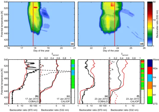
Fig. 3. Results from the microphysical column model ZOMM driven by ERA-Interim based CLaMS trajectories with superimposed
small-scale temperature fluctuations. Upper panels (a, d): time series of backscatter ratios (BSR) at 532 nm (color coded); vertical red lines: S1 and S2. Lower panels: comparison between simulations (red) and measurements (black), namely COBALD BSR at 870 nm (b, e) and CALIOP BSR (solid) and depolarization (dashed) at 532 nm (c, f). Simulations (red lines) in (c) and (f) have been interpolated corresponding to the vertical resolution of the instrument. Color bars: PSC classification scheme according to Pitts et al. (2011) for CALIOP observations. CALIOP data are from orbits 2010-01-18T00-19-57Z (c) and 2010-01-24T01-22-07Z (f) closest to Sodankylä.
performed various simulations with different initial condi-tions and model configuracondi-tions. The results with the best agreement between simulated and observed PSC properties are shown in Figs. 3 and 4. This simulation accounted for ho-mogeneous ice nucleation, heterogeneous nucleation of NAT and ice on foreign nuclei as well as the nucleation of ice on preexisting NAT particles and the nucleation of NAT on pre-existing ice particles. Small-scale temperature fluctuations, as described in Sect. 2.3.1, needed to be superimposed onto the trajectories in order to reproduce the observations.
4.1 Direct measurement–model comparison
The comparison of measured and simulated optical proper-ties, namely BSR andδaerosol, is presented in Fig. 3. Here,
the modeled temporal evolution of BSR at 532 nm along the trajectories is shown in panels a and d as a function of potential temperature. Figure 4 presents the correspond-ing results for water vapor. We started trajectories backward and forward in time as described in Sect. 2.3 along the de-scent of S1 (FLASH-B and COBALD) and the ade-scent of S2 (CFH and COBALD). The operation schedule of FLASH-B and CFH and a discussion about the data quality dur-ing ascent and descent can be found in our companion pa-per (Khaykin et al., 2013). The simulated vertical profiles
have been compared to balloon- and satellite-borne measure-ments. Their approximate observation time is indicated by vertical red lines in the upper panels. Their exact position is equal to the position of S1 and S2 in each case. Panel b shows modeled and observed values for the initial sounding S1 on 17 January and panel e for S2, the sounding which took place on 23 January 2010. Panels c and f show satellite mea-surements, a 25 km mean around the profile closest in time and space to the corresponding balloon sounding from So-dankylä. Whereas CALIPSO and Aura were∼500 km away
from Sodankylä with a time difference of 3 h between the in-dividual measurements on 17 January, measurements on the 23 January have a horizontal displacement of only∼100 km
but a 6 h time lag. All measurements are shown in black, sim-ulations in red. The simulated profiles in panels c and f are interpolated to the corresponding grid of CALIOP and MLS and smoothed with a moving average filter spanning 3.1 km for the comparison with MLS.
Day of the year
(d)
22 23 24 25 26
H2
O [ppmv]
4 4.5 5 5.5
4 5 6
H
2O [ppmv]
(e)
23 Jan 2010 CFH
4 5 6
H
2O [ppmv]
(f)
23 Jan 2010 Aura MLS Day of the year
Potential temperature [K]
(a)
16 17 18 19 20 21
400 420 440 460 480 500 520 540
4 5 6
400 420 440 460 480 500 520 540
Potential temperature [K]
H
2O [ppmv]
(b)
17 Jan 2010 FLASH−B
H
2O [ppmv]
(c)
17 Jan 2010 Aura MLS
4 5 6
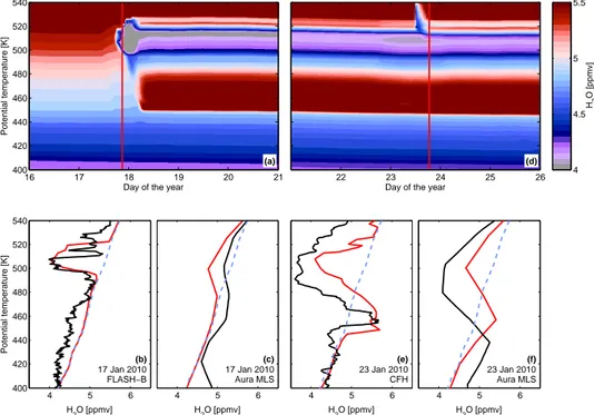
Fig. 4. Results from the microphysical column model ZOMM driven by ERA-Interim based CLaMS trajectories with superimposed
small-scale temperature fluctuations. Upper panels (a, d): time series of water vapor mixing ratios (color coded); vertical red lines: S1 and S2. Lower panels: comparison between simulations (red) and measurements (black), namely FLASH-B (b), CFH (e) and MLS (c, f). Simulations (red lines) in (c) and (f) have been smoothed and interpolated corresponding to the vertical resolution of the instrument. Blue dashed line in lower panels (b, c, e, f): climatological mean water vapor profile. MLS data are interpolated to orbits 2010-01-18T00-19-57Z (c) and 2010-01-24T01-22-07Z (f) closest to Sodankylä.
beginning of the simulation. Within the first 48 h after the start of the simulation, a significant enhancement in BSR in-dicates the formation of a cloud. Att∼17.5 days,
temper-atures become low enough to permit first NAT nucleation on preexisting particle surfaces. NAT number densities of 10−3cm−3lead to a small but visible increase in BSR. With
decreasing temperatures, STS particles grow through uptake of H2O (as shown by the slightly decreasing water vapor
mixing ratios in Fig. 4) and HNO3 (Fig. 7) from the gas
phase and contribute significantly to a continuous increase of BSR. The onset of clearly reduced water vapor mixing ratios shortly before the point of observation is shown in Fig. 4 and marks the formation of ice particles. The com-parison between simulated vertical backscatter profiles (red) with those measured by COBALD (black line in Fig. 3b) shows a reasonable agreement. However, small-scale struc-tures of enhanced BSR seen by COBALD are only partly reflected and BSR values stay below the maximum detected by COBALD. BSR values as large as 200 (at 870 nm) may be simulated by choosing a slightly different phase of a fluc-tuation as seen in the presentation of the ensemble runs be-low. As Fig. 3c shows, CALIOP measurements (black line) are represented extremely well. Simulatedδaerosolvalues are
enhanced in the same altitude region as in the CALIOP ob-servations, but values ofδaerosolmeasured by CALIOP
fluc-tuate more strongly, producing “jumps” between the ice and STS class (compare dashed lines in Fig. 3c). Even though instrumental noise and the lower resolution might be an ex-planation for this behavior, COBALD measures large fluc-tuations in BSR, which suggests changes in the underlying cloud composition, too. A profound anti-correlation between the profiles of BSR and H2O (black lines in Fig. 3b and
Fig. 4b, respectively) strengthens the reliability of the two in-dependent measurements. Enhancements in BSR and a cor-responding depletion in the vapor phase, both strongly lay-ered, suggests an ice cloud. The small color bar next to the vertical profiles denotes the results from the CALIOP parti-cle classification scheme and supports the existence of dis-tinct layers of ice embedded in a broader liquid PSC. A de-tailed discussion of the BSR and water vapor measurements together with a presentation of both within the same plot can be found in Khaykin et al. (2013). Simulated ice number den-sities in the core of the cloud lie between 10−3cm−3 and
10−2cm−3, leading to a maximum BSR at 532 nm of almost
7. In Fig. 3a, downwind of S1, homogeneous ice nucleation sets in and higher ice number densities between 0.1 cm−3and
1 cm−3are simulated. Those high number densities cause an
Potential temperature [K] 400 440 470 500 540
T − T
frost
[K]
−4 −3 −2 −1 0 1 2 3 4
Potential temperature [K] 400 440 470 500 540
Temperature [K]
184 188 192 196
Homogeneous nucleation
Potential temperature [K] 400 440 470 500 540
Potential temperature [K] 400 440 470 500 540
Potential temperature [K] 400 440 470 500 540
Potential temperature [K] 400 440 470 500 540
Day of the year
Potential temperature [K]
17 17.5 18 18.5 19 400
440 470 500 540
Heterogeneous nucleation
Day of the year 17 17.5 18 18.5 19
Homogeneous nucleation Temperature fluctuations
Day of the year 17 17.5 18 18.5 19
Heterogeneous nucleation Temperature fluctuations
Backscatter ratio (532 nm)
1 5 10 50
Number density (ice) [cm
−3
]
1e−4 1e−3 1e−2 1e−1 1 10
Radius (ice) [
µ
m]
0 2 4 6 8 10 12
Number density (NAT) [cm
−3
]
1e−4 1e−3 1e−2 1e−1 1 10
Day of the year 17 17.5 18 18.5 19
Radius (NAT) [
µ
m]
0 2 4 6 8 10 12
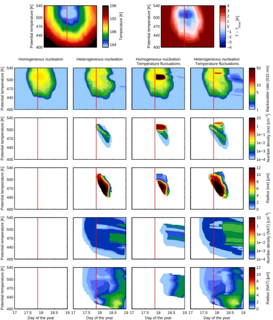
Fig. 5. Results from the microphysical column model ZOMM driven by ERA-Interim based CLaMS trajectories (17–19 January 2010).
Vertical red line: S1. Top panels: ERA-Interim temperatures (temperature correction applied) shown as absolute temperature (left panel) and relative to the frost point temperature (Tfrost), which has been calculated from the climatological mean water vapor profile (right panel). Rows:
backscatter ratios at 532 nm, ice and NAT number densities and radii. Columns show four different scenarios: column 1 – only homogeneous nucleation of ice, no superimposed temperature fluctuations; column 2 – same, but in addition allow for heterogeneous nucleation; column 3 – only homogeneous nucleation of ice, but with superimposed small-scale temperature fluctuations; column 4 – with both, heterogeneous nucleation and superimposed temperature fluctuations. Homogeneous simulations include homogeneous ice nucleation and NAT nucleation on preexisting ice particles only. Heterogeneous model runs also include heterogeneous ice and NAT nucleation on foreign nuclei.
much smaller. This tail consists of NAT particles (see Fig. 5) that nucleated on the ice cloud, forming a NAT cloud of class “Mix2” and “Mix2-enh”, as first described by Carslaw et al. (1998a).
The magnitude of the H2O reduction in the gas phase
ob-served by FLASH-B is roughly captured by the simulations. Again, fine-scale structures are not reproduced by the model (Fig. 4b). The resolution of MLS is too coarse to capture the local reduction in H2O at this time (Fig. 4c). Ice particles
evaporate already 12 h after the FLASH-B observation and a clear and permanent redistribution of H2O becomes visible
att∼18.5 days in Fig. 4a, and it remains visible until the end of the simulation.
Close to the second observation, temperatures drop again and reach values almost as cold as on the 17 January. How-ever, the reduction in H2O prevents the formation of ice
CALIOP (3 at 532 nm) would not suggest an ice cloud. Val-ues of BSR remain smaller than they were on 17 January and CALIOP observations suggest a predominantly liquid cloud with few embedded NAT particles. The NAT signal is partially obscured by the strong STS signal (Fig. 3f). The comparison between modeled and observed H2O reveals that
even though the model captures signatures of de- and rehy-dration, the vertical extent of the dehydrated air remains too small in the simulation. The simulated maximum reduction in water vapor of 1.4 ppm at 514 K is almost as large as ob-served by CFH. However, the dehydrated region is smaller in vertical extent and ranges only from 485 K to 525 K. A pos-sible explanation of the underestimated vertical extent of de-hydrated air in the simulation might again be the tempera-ture profile. Figure 2b shows that ERA-Interim temperatempera-tures are also too warm compared to the observation at the top of the sounding, which prevents the formation of ice particles above 525 K. The resulting availability of H2O at high
alti-tudes offers the possibility for ice formation on the 23 Jan-uary 2010 in our simulation, whereas CALIOP observations documented the last ice clouds in the vortex on 21 January (Pitts et al., 2011).
Whereas ZOMM underestimates the vertical extent of the dehydrated air, it overestimates the dimension of the rehy-drated signature. This is related to uncertainties of the H2O
profile used to initialize the model and/or to wind shear (hor-izontal shear is unimportant due to the constraint of the ro-tating air in the vortex, but vertical shear is significant). The column model is rigorously mass-conserving. However, in-dependent of temperatures and the nucleation mechanism, ZOMM cannot simultaneously reproduce both, the de- and rehydration signatures observed by CFH relative to the as-sumed initial H2O profile. Inspection of Fig. 2 of Khaykin
et al. (2013) reveals the day-to-day variability between the individual water vapor profiles. Whereas the agreement be-tween the measurement and the mean values is almost perfect in undisturbed air masses below 450 K on 22 January 2010, there is variability on 17 and 23 January 2010. A different initial profile on these days could be consistent with mass-balanced profiles in the observations. Nevertheless, such pro-files remain speculative and we refrained from changing the initial profile for model improvement, while the observed profiles could be affected by wind shear. A three-dimensional treatment of the wind fields, which also includes wind shear and mixing of air masses, would be required (but with such a model, additional uncertainties would be introduced and the detailed microphysics could hardly be tested). These issues hardly impact the results for S1 during the short (2-day) run-up of the model, whereas they clearly affect S2. Nevertheless, the different scenarios discussed in the subsequent paragraph and presented in Fig. 5 and Fig. 6 are robust and allow clear conclusions.
Figure 5 compares simulations using four different scenar-ios. The top panels show ERA-Interim temperatures, which were corrected according to the measured temperature
pro-file of S1 (compare Sect. 2.3 and Fig. 2) and provide the basis for all four simulations. The simulated profiles at S1 and S2 can be seen for each scenario in Fig. 6 together with the observations. Figure 6 will be explained and discussed in detail in Sect. 4.2. The first scenario (Fig. 5, 1st column), which accounts only for homogeneous ice nucleation, cannot explain the observations at all. Supersaturations with respect to ice remain too small and since no ice particles form, NAT particles cannot form either. The second scenario (Fig. 5, 2nd column), which includes heterogeneous nucleation of ice and NAT particles according to Engel et al. (2013) and Hoyle et al. (2013), changes the model results completely. Ice su-persaturations are sufficient for heterogeneous nucleation of 10−3cm−3ice particles. Within a short time, these particles
grow to sizes>12 µm in radius. With a settling velocity
be-tween 100 m h−1 and 200 m h−1, ice particles can sediment
up to 2 km before evaporation. The third scenario (Fig. 5, 3rd column) shows that the superposition of small-scale tem-perature fluctuations on the synoptic trajectories leads to ice formation even in the homogeneous freezing case. However, this result does not agree with the observations, because the nucleation of high ice number densities (between 1 cm−3and
10 cm−3) prevents the growth of ice particles to sizes which
could sediment fast enough to achieve a satisfying agree-ment with the water vapor observations (maximum sedimen-tation distances of only a few hundred meters). The final sce-nario (Fig. 5, 4th column) includes both heterogeneous nu-cleation and superimposed small-scale temperature fluctua-tions. The inclusion of heterogeneous nucleation in this sim-ulation causes NAT to form prior to ice. Consequently, those NAT particles are assumed to be enclosed by ice and redis-tributed by the subsequent growth and sedimentation of the ice particles. We will discuss this point further below. Addi-tionally, the nucleation of ice particles starts earlier than in all other cases and the fluctuations enable a larger ice cloud area to be generated.
4.2 Ensemble calculations for stochastic impact of temperature fluctuations
Homogeneous nucleation
Backscatter ratio (870 nm)
Potential temperature [K]
1 5 10 50 100
400 420 440 460 480 500 520 540
Potential temperature [K]
∆ H
2O [ppmv]
−1.5 −0.75 0 0.75 1.5
400 420 440 460 480 500 520 540
Heterogeneous nucleation
Backscatter ratio (870 nm)
1 5 10 50 100
∆ H
2O [ppmv]
−1.5 −0.75 0 0.75 1.5
Homogeneous nucleation Temperature fluctuations
Backscatter ratio (870 nm)
1 5 10 50 100
∆ H
2O [ppmv]
−1.5 −0.75 0 0.75 1.5
Heterogeneous nucleation Temperature fluctuations
Backscatter ratio (870 nm)
1 5 10 50 100
∆ H
2O [ppmv]
−1.5 −0.75 0 0.75 1.5
Fig. 6. Comparison between measured and simulated profiles of backscatter ratios (BSR) for S1 (upper row) and water vapor mixing ratios
for S2 (lower row). Mixing ratios are expressed as deviation from the climatological mean water vapor profile. The four different model scenarios are the same as in Fig. 5. Black line: COBALD (upper row) and CFH (lower row) measurements. Gray shaded area: variations caused by different small-scale temperature fluctuations modeled by an ensemble with 10 members. Red line: model results for the best fluctuation member shown in Figs. 3–5. Dashed line: model results obtained without temperature correction (as shown in Fig. 2).
the fluctuations. Cirisan et al. (2013) have performed similar calculations for cirrus clouds.
Figure 6 presents a comparison of profiles of BSR and
1H2O for various scenarios with and without heterogeneous
nucleation and with 10 different sets of small-scale temper-ature fluctuations. BSR profiles for 17 January are presented in the upper four panels,1H2O profiles for 23 January are
shown in the lower four panels. The model results, which have already been described above and shown in Figs. 3–5, correspond to the red curves while the other nine members are shown as gray shaded areas. The red curves also repre-sent the particular member which produced the best agree-ment with the measureagree-ments in terms of dehydration.
As expected, no signatures of de- or rehydration are visible if only homogeneous ice nucleation and synoptic-scale tem-peratures are applied. The lower row shows that an improved agreement between CFH and the simulation can only be achieved if heterogeneous ice nucleation or small-scale tem-perature fluctuations are included, or both. However, when heterogeneous nucleation is included but not the small-scale temperature fluctuations (2nd column), modeled values of BSR remain too small in comparison with COBALD BSR values. Conversely, combining homogeneous nucleation and the superposition of small-scale temperature fluctuations im-proves the modeled backscatter, but generates an irregular
and 18 January 2010. However, a certain scatter of BSRs still exists, possibly originating from temperature perturbations, much like what is seen in the model results when a range of temperature fluctuations is used.
Finally, to demonstrate the need for the temperature cor-rection depicted in Fig. 2b and c, we included, as dashed black lines in Fig. 6, model results based on the origi-nal ERA-Interim trajectories with and without superimposed small-scale temperature fluctuations. The only simulation which produced any dehydration signal is the one combin-ing heterogeneous nucleation with temperature fluctuations. However, the modeled dehydration is much smaller than that observed.
4.3 Relevance for denitrification
Denitrification plays an important role in ozone loss by slow-ing the conversion of chlorine radicals back into reservoir species. This process may cause an enhancement of ozone destruction and can lead to increased accumulated ozone losses over the course of the winter (e.g., Müller et al., 1994). Denitrification is particularly important in the Arctic with its warmer temperatures (e.g., Chipperfield and Pyle, 1998) and severe denitrification has been a major factor in bringing about the record ozone loss in the Arctic winter 2010/2011 (Manney et al., 2011; Pommereau et al., 2013).
Recent observations suggest the possibility of heteroge-neous ice nucleation on preexisting NAT particles. Pitts et al. (2011) observed an increase in synoptic-scale ice PSCs con-comitant with decreasing number densities of NAT mixtures in January 2010. Such a process would imply that the sedi-mentation of ice particles not only dehydrates but also deni-trifies the stratosphere due to the removal of HNO3.
Khos-rawi et al. (2011) investigated this hypothesis and offered ice nucleation on NAT particles as a possible explanation for the low HNO3observations by the Sub-Millimetre
Radiome-ter (SMR) aboard the Odin satellite and Aura/MLS during the same winter. However, the present modeling study re-veals that dehydration and denitrification are not necessar-ily related to each other. The observed case does not signifi-cantly contribute to the overall denitrification for the follow-ing reasons. At the start of the simulations, before ice for-mation, the nucleation of NAT on foreign nuclei accounts for NAT number densities of 10−3cm−3, but the effective
radius of NAT particles formed along the trajectories does not exceed 2 µm. The amount of HNO3condensing on these
NAT particles is negligible, namely less than 10 % of the to-tal available HNO3, while the major fraction of HNO3
re-sides in the liquid droplets. This results in a depletion in the gas phase HNO3 (see denoxification in Fig. 7a) and
decel-erates the growth of the NAT particles (see Fig. 4 in Voigt et al., 2005). Next, ice nucleates, partly on the preexisting NAT, and HNO3also co-condenses on the growing ice
par-ticles, which sediment and dehydrate efficiently. However, the resulting denitrification is minor, as most of the mass
of the falling particles is composed of water molecules. Af-ter the ice has evaporated, NAT particles are released and would have the chance to denitrifiy the air, if they could sur-vive long enough to grow. However, the air warms rapidly fromT < Tfrost toT > TNAT(see Fig. 1) and does not stay
in the intervalTNAT−5 K< T < TNAT−2 K, which is most
efficient for denitrification (Voigt et al., 2005), for a suffi-cient amount of time. The resulting denitrification signal in Fig. 7b shows redistributions of HNO3over small height
dif-ferences, but no strong, coherent denitrification. This impres-sion is independent of the nucleation scenario or the phase of the temperature fluctuation and, thus, very robust. Instead, the strong denitrification of the Arctic winter 2009/2010 oc-curred during the first half of January, that is, before the onset of synoptic-scale ice clouds, and was likely caused by NAT clouds downwind of mountain wave ice PSCs, which can act as mother clouds for so-called NAT rocks (Fueglistaler et al., 2002). Evidence of this can be seen in the Odin/SMR and Aura/MLS satellite measurements of HNO3shown in Fig. 3
of Khosrawi et al. (2011). In the beginning of January 2010, gas phase mixing ratios of HNO3decreased significantly at
high altitudes and remained low until the end of February. Below 50 hPa, a concurrent HNO3increase is visible in the
data, which allows the conclusion that a permanent, verti-cal redistribution of HNO3may have taken place. Minimum
values of gas phase HNO3 were observed by Aura/MLS in
the second half of January at the same time than CALIOP confirmed the existence of synoptic-scale ice clouds. How-ever, the renitrified layer below showed no further increase in HNO3. Instead, HNO3 mixing ratios above 50 hPa
in-creased again with proceeding time and increasing tempera-tures. Hence, we expect denoxification and no additional de-and renitrification at this time in the winter. Recent CLaMS simulations show a similar picture with HNO3fluxes largest
in the first half of January (Grooß et al., 2014). For this rea-son, we cannot confirm the suggestion by Khosrawi et al. (2011), namely that the observed denitrification was linked to ice particle formation on NAT during the synoptic cool-ing event in mid-January. This case study indicates that the conditions that led to the observed dehydration in the second half of January 2010 would not support sufficient growth of NAT particles to lead to significant denitrification.
5 Discussion and conclusions
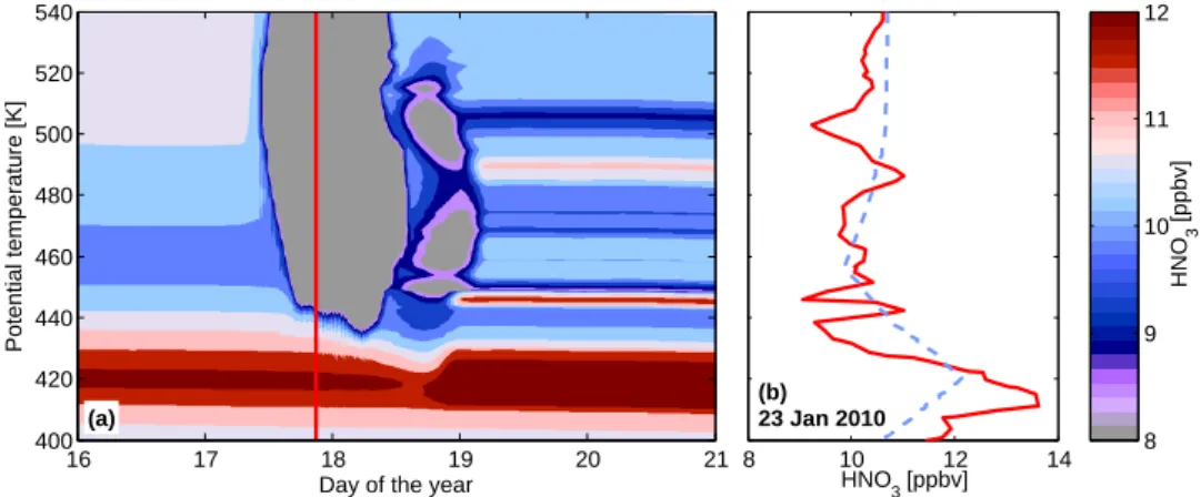
Day of the year
Potential temperature [K]
(a)
16 17 18 19 20 21
400 420 440 460 480 500 520 540
HNO
3
[ppbv]
8 9 10 11 12
8 10 12 14
HNO 3 [ppbv] (b)
23 Jan 2010
Fig. 7. Results from the microphysical column model ZOMM driven by ERA-Interim based CLaMS trajectories with superimposed
small-scale temperature fluctuations. (a) Time series of gas phase nitric acid mixing ratios (color coded); vertical red line: S1. (b) Simulated total nitric acid profile (red) at S2 compared to the initial nitric acid profile (blue dashed).
profiles agree reasonably with CFH and FLASH-B carried by the balloon sondes and with MLS satellite measurements. Optical T-Matrix calculations enabled the direct comparison of the simulations with COBALD and CALIOP backscatter measurements. To this end, we examined the effect of small-scale temperature fluctuations and compared homogeneous vs. heterogeneous formation of ice particles.
It was demonstrated that heterogeneous nucleation of ice is essential to reproduce the observed de- and rehydration signatures. Even though ERA-Interim temperatures along the trajectories had to be lowered by up to 1.5 K in order to obtain agreement with the temperatures measured by the sondes, temperatures stayed aboveTfrost−3 K, which is the
temper-ature required for homogeneous nucleation of ice in ternary solution droplets. Small-scale temperature fluctuations addi-tionally lowered the temperature, caused higher supersatu-rations and therefore enabled the formation of ice clouds, even when homogeneous ice nucleation was the only allowed ice formation pathway. However, homogeneous nucleation at high supersaturations resulted in ice formation with the characteristics of wave clouds: high number densities of par-ticles remain too small to sediment and cannot explain the observed vertical redistribution of water. In contrast, hetero-geneous ice nucleation takes place at lower supersaturations, causing a selective freezing of only a few ice crystals. Those particles can grow to sizes large enough (r &10 µm) to settle
fast and reproduce the signatures of de- and rehydration. Even though small-scale temperature fluctuations are not required to achieve de- and renitrification in the present case, the resulting PSC backscatter is too low without small-scale temperature fluctuations, and rapid cooling rates help to improve the agreement with the COBALD measurements. However, the two balloon soundings provide only snapshots of the atmosphere, which depend on the precise tempera-ture variations not only at the point of observation, but also upstream along the air parcel trajectories. Discrepancies
be-tween ERA-Interim temperature fields and measured temper-atures were found, which we needed to correct. Whereas So-dankylä, located at the edge of the cold pool, is characterized by temperatures just belowTfrost and is therefore very
sen-sitive to the smallest of temperature changes, the CALIOP measurements show large areas deeper in the vortex with persistent synoptic-scale ice clouds. The observed dehydra-tion above Sodankylä, not only on 23 January but also a few days earlier and later (as shown by Khaykin et al., 2013), is most likely caused by such large-scale fields of persistent ice clouds and not by the observed small-scale structures above Sodankylä. The fact that the reduction in H2O measured by
CFH is not balanced by the rehydration layer below suggests that wind shear and subsequent mixing of air masses have affected the observed profile. An accurate estimate of these effects can only be made using a three-dimensional modeling approach.
Acknowledgements. This work was supported by the European
Commission Seventh Framework Programme (FP7) under the grant number RECONCILE-226365-FP7-ENV-2008-1. Support for C. R. Hoyle was obtained from the Swiss National Science Founda-tion (SNSF) under the grant numbers 200021_120175/1 (Modelling Heterogeneous and Homogeneous Ice Nucleation and Growth at Cirrus Cloud Levels) and 200021_140663 (Modelling of aerosol effects in mixed-phase clouds). Partial support for S. M. Khaykin received by the Russian Foundation for Basic Research (grant numbers 12-05-31384 and 11-05-00475). Water vapor and aerosol soundings in Sodankylä were partially supported by the Finnish Academy under grant number 140408. Aura MLS gas species data were provided courtesy of the MLS team and obtained through the Aura MLS website (http://mls.jpl.nasa.gov/index-eos-mls.php). Particular gratitude to Alexey Lykov (CAO) who carried out FLASH-B flight on 17 January 2010.
References
Brabec, M., Wienhold, F. G., Luo, B. P., Vömel, H., Immler, F., Steiner, P., Hausammann, E., Weers, U., and Peter, T.: Particle backscatter and relative humidity measured across cirrus clouds and comparison with microphysical cirrus modelling, Atmos. Chem. Phys., 12, 9135–9148, doi:10.5194/acp-12-9135-2012, 2012.
Bukowiecki, N., Zieger, P., Weingartner, E., Jurányi, Z., Gysel, M., Neininger, B., Schneider, B., Hueglin, C., Ulrich, A., Wichser, A., Henne, S., Brunner, D., Kaegi, R., Schwikowski, M., To-bler, L., Wienhold, F. G., Engel, I., Buchmann, B., Peter, T., and Baltensperger, U.: Ground-based and airborne in-situ measure-ments of the Eyjafjallajökull volcanic aerosol plume in Switzer-land in spring 2010, Atmos. Chem. Phys., 11, 10011–10030, doi:10.5194/acp-11-10011-2011, 2011.
Carslaw, K. S., Wirth, M., Tsias, A., Luo, B. P., Dörnbrack, A., Leutbecher, M., Volkert, H., Renger, W., Bacmeister, J. T., and Peter, T.: Particle microphysics and chemistry in remotely ob-served mountain polar stratospheric clouds, J. Geophys. Res., 103, 5785–5796, doi:10.1029/97JD03626, 1998a.
Carslaw, K. S., Wirth, M., Tsias, A., Luo, B. P., Dörnbrack, A., Leutbecher, M., Volkert, H., Renger, W., Bacmeister, J. T., Reimer, E., and Peter, T.: Increased stratospheric ozone deple-tion due to mountain-induced atmospheric waves, Nature, 391, 675–678, doi:10.1038/35589, 1998b.
Chipperfield, M. P. and Pyle, J. A.: Model sensitivity studies of Arctic ozone depletion, J. Geophys. Res., 103, 28389–28403, doi:10.1029/98JD01960, 1998.
Cirisan, A., Luo, B. P., Engel, I., Wienhold, F. G., Krieger, U. K., Weers, U., Romanens, G., Levrat, G., Jeannet, P., Ruffieux, D., Philipona, R., Calpini, B., Spichtinger, P., and Peter, T.: Balloon-borne match measurements of mid-latitude cirrus clouds, Atmos. Chem. Phys. Discuss., 13, 25417–25479, doi:10.5194/acpd-13-25417-2013, 2013.
Dee, D. P., Uppala, S. M., Simmons, A. J., Berrisford, P., Poli, P., Kobayashi, S., Andrae, U., Balmaseda, M. A., Balsamo, G., Bauer, P., Bechtold, P., Beljaars, A. C. M., van de Berg, L., Bid-lot, J., Bormann, N., Delsol, C., Dragani, R., Fuentes, M., Geer, A. J., Haimberger, L., Healy, S. B., Hersbach, H., Hólm, E. V., Isaksen, L., Kållberg, P., Köhler, M., Matricardi, M., McNally, A. P., Monge-Sanz, B. M., Morcrette, J.-J., Park, B.-K., Peubey, C., de Rosnay, P., Tavolato, C., Thépaut, J.-N., and Vitart, F.: The ERA-Interim reanalysis: configuration and performance of the data assimilation system, Q. J. Roy. Meteor. Soc., 137, 553–597, doi:10.1002/qj.828, 2011.
Drdla, K., Schoeberl, M. R., and Browell, E. V.: Microphysical modeling of the 1999-2000 Arctic winter: 1. Polar stratospheric clouds, denitrification, and dehydration, J. Geophys. Res., 107, SOL 55-1–SOL 55-21, doi:10.1029/2001JD000782, 2002. Dye, J. E., Baumgardner, D., Gandrud, B. W., Kawa, S. R., Kelly,
K. K., Loewenstein, M., Ferry, G. V., Chan, K. R., and Gary, B. L.: Particle Size Distributions in Arctic Polar Stratospheric Clouds, Growth and Freezing of Sulfuric Acid Droplets, and Implications for Cloud Formation, J. Geophys. Res., 97, 8015– 8034, doi:10.1029/91JD02740, 1992.
Engel, I., Luo, B. P., Pitts, M. C., Poole, L. R., Hoyle, C. R., Grooß, J.-U., Dörnbrack, A., and Peter, T.: Heterogeneous formation of polar stratospheric clouds – Part 2: Nucleation of ice on synoptic
scales, Atmos. Chem. Phys., 13, 10769–10785, doi:10.5194/acp-13-10769-2013, 2013.
Fahey, D. W., Kelly, K. K., Kawa, S. R., Tuck, A. F., Loewenstein, M., Chan, K. R., and Heidt, L. E.: Observations of denitrification and dehydration in the winter polar stratospheres, Nature, 344, 321–324, doi:10.1038/344321a0, 1990.
Flentje, H., Dörnbrack, A., Fix, A., Meister, A., Schmid, H., Fueglistaler, S., Luo, B. P., and Peter, T.: Denitrification inside the stratospheric vortex in the winter of 1999–2000 by sedimen-tation of large nitric acid trihydrate particles, J. Geophys. Res., 107, AAC 11-1–AAC 11-15, doi:10.1029/2001JD001015, 2002. Fueglistaler, S., Luo, B. P., Voigt, C., Carslaw, K. S., and Peter, T.: NAT-rock formation by mother clouds: a microphysical model study, Atmos. Chem. Phys., 2, 93–98, doi:10.5194/acp-2-93-2002, 2002.
Fueglistaler, S., Buss, S., Luo, B. P., Wernli, H., Flentje, H., Hostetler, C. A., Poole, L. R., Carslaw, K. S., and Peter, T.: De-tailed modeling of mountain wave PSCs, Atmos. Chem. Phys., 3, 697–712, doi:10.5194/acp-3-697-2003, 2003.
Gary, B. L.: Mesoscale temperature fluctuations in the stratosphere, Atmos. Chem. Phys., 6, 4577–4589, doi:10.5194/acp-6-4577-2006, 2006.
Grooß, J.-U., Engel, I., Borrmann, S., Frey, W., Günther, G., Hoyle, C. R., Kivi, R., Luo, B. P., Molleker, S., Peter, T., Pitts, M. C., Schlager, H., Stiller, G., Vömel, H., Walker, K. A., and Müller, R.: Nitric acid trihydrate nucleation and denitrification in the Arctic stratosphere, Atmos. Chem. Phys., 14, 1055–1073, doi:10.5194/acp-14-1055-2014, 2014.
Hoyle, C. R., Luo, B. P., and Peter, T.: The origin of high ice crystal number densities in cirrus clouds, J. Atmos. Sci., 62, 2568–2579, doi:10.1175/JAS3487.1, 2005.
Hoyle, C. R., Engel, I., Luo, B. P., Pitts, M. C., Poole, L. R., Grooß, J.-U., and Peter, T.: Heterogeneous formation of polar stratospheric clouds – Part 1: Nucleation of nitric acid trihydrate (NAT), Atmos. Chem. Phys., 13, 9577–9595, doi:10.5194/acp-13-9577-2013, 2013.
Jimenez, C., Pumphrey, H. C., MacKenzie, I. A., Manney, G. L., Santee, M. L., Schwartz, M. J., Harwood, R. S., and Wa-ters, J. W.: EOS MLS observations of dehydration in the 2004-2005 polar winters, Geophys. Res. Lett., 33, L16806, doi:10.1029/2006GL025926, 2006.
Kärcher, B. and Lohmann, U.: A parameterization of cirrus cloud formation: Heterogeneous freezing, J. Geophys. Res., 108, 4402, doi:10.1029/2002JD003220, 2003.
Kelly, K. K., Tuck, A. F., Murphy, D. M., Proffitt, M. H., Fahey, D. W., Jones, R. L., McKenna, D. S., Loewenstein, M., Podolske, J. R., Strahan, S. E., Ferry, G. V., Chan, K. R., Vedder, J. F., Gregory, G. L., Hypes, W. D., McCormick, M. P., Browell, E. V., and Heidt, L. E.: Dehydration in the lower Antarctic stratosphere during late winter and early spring, 1987, J. Geophys. Res., 94, 11 317–11 357, doi:10.1029/JD094iD09p11317, 1989.
Khosrawi, F., Urban, J., Pitts, M. C., Voelger, P., Achtert, P., Kaphlanov, M., Santee, M. L., Manney, G. L., Murtagh, D., and Fricke, K.-H.: Denitrification and polar stratospheric cloud for-mation during the Arctic winter 2009/2010, Atmos. Chem. Phys., 11, 8471–8487, doi:10.5194/acp-11-8471-2011, 2011.
Kley, D. and Stone, E. J.: Measurement of water vapor in the strato-sphere by photo dissociation with Ly-Alpha (1216 A) light, Rev. Sci. Instrum., 49, 691–697, doi:10.1063/1.1135596, 1978. Koop, T., Biermann, U. M., Raber, W., Luo, B. P., Crutzen,
P. J., and Peter, T.: Do stratospheric aerosol droplets freeze above the ice frost point?, Geophys. Res. Lett., 22, 917–920, doi:10.1029/95GL00814, 1995.
Koop, T., Luo, B. P., Tsias, A., and Peter, T.: Water activity as the determinant for homogeneous ice nucleation in aqueous solu-tions, Nature, 406, 611–614, doi:10.1038/35020537, 2000. Krieger, U. K., Mössinger, J. C., Luo, B. P., Weers, U., and Peter, T.:
Measurement of the Refractive Indices of H2SO4-HNO3-H2O
Solutions to Stratospheric Temperatures, Appl. Opt., 39, 3691– 3703, doi:10.1364/AO.39.003691, 2000.
Lambert, A., Read, W. G., Livesey, N. J., Santee, M. L., Manney, G. L., Froidevaux, L., Wu, D. L., Schwartz, M. J., Pumphrey, H. C., Jimenez, C., Nedoluha, G. E., Cofield, R. E., Cuddy, D. T., Daffer, W. H., Drouin, B. J., Fuller, R. A., Jarnot, R. F., Knosp, B. W., Pickett, H. M., Perun, V. S., Snyder, W. V., Stek, P. C., Thurstans, R. P., Wagner, P. A., Waters, J. W., Jucks, K. W., Toon, G. C., Stachnik, R. A., Bernath, P. F., Boone, C. D., Walker, K. A., Urban, J., Murtagh, D., Elkins, J. W., and Atlas, E.: Vali-dation of the Aura Microwave Limb Sounder middle atmosphere water vapor and nitrous oxide measurements, J. Geophys. Res., 112, D24S36, doi:10.1029/2007JD008724, 2007.
Lambert, A., Santee, M. L., Wu, D. L., and Chae, J. H.: A-train CALIOP and MLS observations of early winter Antarctic polar stratospheric clouds and nitric acid in 2008, Atmos. Chem. Phys., 12, 2899–2931, doi:10.5194/acp-12-2899-2012, 2012.
Livesey, N. J., Read, W. G., Froidevaux, L., Lambert, A., Man-ney, G. L., Pumphrey, H. C., Santee, M. L., Schwartz, M. J., Wang, S., Cofield, R. E., Cuddy, D. T., Fuller, R. A., Jarnot, R. F., Jiang, J. H., Knosp, B. W., Stek, P. C., Wagner, P. A., and Wu, D. L.: Version 3.3 Level 3 data quality and description document, Tech. Rep. JPL D-33509, Jet Propulsion Laboratory, http://mls.jpl.nasa.gov, last access: 15 January 2013, 2011. Luo, B. P., Peter, T., Fueglistaler, S., Wernli, H., Wirth, M., Kiemle,
C., Flentje, H., Yushkov, V. A., Khattatov, V., Rudakov, V., Thomas, A., Borrmann, S., Toci, G., Mazzinghi, P., Beuer-mann, J., Schiller, C., Cairo, F., Di Donfrancesco, G., Adri-ani, A., Volk, C. M., Strom, J., Noone, K., Mitev, V., MacKen-zie, R. A., Carslaw, K. S., Trautmann, T., Santacesaria, V., and Stefanutti, L.: Dehydration potential of ultrathin clouds at the tropical tropopause, Geophys. Res. Lett., 30, 1557, doi:10.1029/2002GL016737, 2003a.
Luo, B. P., Voigt, C., Fueglistaler, S., and Peter, T.: Extreme NAT su-persaturations in mountain wave ice PSCs: A clue to NAT forma-tion, J. Geophys. Res., 108, 4441, doi:10.1029/2002JD003104, 2003b.
Manney, G. L., Santee, M. L., Rex, M., Livesey, N. J., Pitts, M. C., Veefkind, P., Nash, E. R., Wohltmann, I., Lehmann, R., Froidevaux, L., Poole, L. R., Schoeberl, M. R., Haffner, D. P., Davies, J., Dorokhov, V., Gernandt, H., Johnson, B., Kivi, R., Kyro, E., Larsen, N., Levelt, P. F., Makshtas, A., McElroy,
C. T., Nakajima, H., Concepcion Parrondo, M., Tarasick, D. W., von der Gathen, P., Walker, K. A., and Zinoviev, N. S.: Un-precedented Arctic ozone loss in 2011, Nature, 478, 469–475, doi:10.1038/nature10556, 2011.
Marcolli, C., Gedamke, S., Peter, T., and Zobrist, B.: Efficiency of immersion mode ice nucleation on surrogates of mineral dust, Atmos. Chem. Phys., 7, 5081–5091, doi:10.5194/acp-7-5081-2007, 2007.
Maturilli, M. and Dörnbrack, A.: Polar stratospheric ice cloud above Spitsbergen, J. Geophys. Res., 111, D18210, doi:10.1029/2005JD006967, 2006.
McKenna, D. S., Konopka, P., Grooß, J.-U., Günther, G., Müller, R., Spang, R., Offermann, D., and Orsolini, Y.: A new Chem-ical Lagrangian Model of the Stratosphere (CLaMS) – 1. For-mulation of advection and mixing, J. Geophys. Res., 107, 4309, doi:10.1029/2000JD000114, 2002.
Meilinger, S. K., Koop, T., Luo, B. P., Huthwelker, T., Carslaw, K. S., Krieger, U., Crutzen, P. J., and Peter, T.: Size-dependent stratospheric droplet composition in lee wave temperature fluc-tuations and their potential role in PSC freezing, Geophys. Res. Lett., 22, 3031–3034, doi:10.1029/95GL03056, 1995.
Mishchenko, M. I., Travis, L. D., and Mackowski, D. W.: T-Matrix Computations of Light Scattering by Nonspherical Particles: A Review (Reprinted from vol 55, pg 535-575, 1996), J. Quant. Spectrosc. Radiat. Transf., 111, 1704–1744, doi:10.1016/0022-4073(96)00002-7, 2010.
Müller, R., Peter, T., Crutzen, P. J., Oelhaf, H., Adrian, G. P., Clar-mann, T., Wegner, A., Schmidt, U., and Lary, D.: Chlorine chem-istry and the potential for ozone depletion in the Arctic strato-sphere in the winter of 1991/92, Geophys. Res. Lett., 21, 1427– 1430, doi:10.1029/94GL00465, 1994.
Murphy, D. M. and Gary, B. L.: Mesosclae Temper-ature Fluctuations and Polar Stratospheric Clouds, J. Atmos. Sci., 52, 1753–1760, doi:10.1175/1520-0469(1995)052<1753:MTFAPS>2.0.CO;2, 1995.
Nedoluha, G. E., Bevilacqua, R. M., Hoppel, K. W., Daehler, M., Shettle, E. P., Hornstein, J. H., Fromm, M. D., Lumpe, J. D., and Rosenfield, J. E.: POAM III measurements of dehydration in the Antarctic lower stratosphere, Geophys. Res. Lett., 27, 1683– 1686, doi:10.1029/1999GL011087, 2000.
Peter, T. and Grooß, J.-U.: Chapter 4: Polar Stratospheric Clouds and Sulfate Aerosol Particles: Microphysics, Denitrification and Heterogeneous Chemistry, in: Stratospheric Ozone De-pletion and Climate Change, Roy. Soc. Chem., 108–144, doi:10.1039/9781849733182-00108, 2012.
Pitts, M. C., Thomason, L. W., Poole, L. R., and Winker, D. M.: Characterization of Polar Stratospheric Clouds with spaceborne lidar: CALIPSO and the 2006 Antarctic season, Atmos. Chem. Phys., 7, 5207–5228, doi:10.5194/acp-7-5207-2007, 2007. Pitts, M. C., Poole, L. R., and Thomason, L. W.: CALIPSO polar
stratospheric cloud observations: second-generation detection al-gorithm and composition discrimination, Atmos. Chem. Phys., 9, 7577–7589, doi:10.5194/acp-9-7577-2009, 2009.
Pitts, M. C., Poole, L. R., Lambert, A., and Thomason, L. W.: An assessment of CALIOP polar stratospheric cloud com-position classification, Atmos. Chem. Phys., 13, 2975–2988, doi:10.5194/acp-13-2975-2013, 2013.