www.ocean-sci.net/6/861/2010/ doi:10.5194/os-6-861-2010
© Author(s) 2010. CC Attribution 3.0 License.
Ocean Science
Estimates of radiance reflected towards the zenith at the surface of
the sea
E. Aas
Department of Geosciences, University of Oslo, Norway
Received: 6 April 2010 – Published in Ocean Sci. Discuss.: 14 June 2010
Revised: 23 August 2010 – Accepted: 20 September 2010 – Published: 5 October 2010
Abstract. Remote sensing of water colour by ship-mounted sensors represents an important tool for the validation of satellite products and the monitoring of water quality. The recorded radiance from the sea has to be corrected for the surface-reflected radiance from sun and sky in order to obtain the water-leaving radiance. Here the simple case of radiance reflected towards the zenith is studied. A set of observed sky radiance and solar irradiance data from Oslo has been used together with a Gaussian slope distribution for the sea sur-face in order to estimate the reflected radiance. The spectral range studied is 405–650 nm, the solar zenith angles are in the range 37◦–76◦, and the wind speeds are up to 10 m s−1. The analysis of the results show that the reflected radiance has to be separated into three contributions: sky radiance and sun rays reflected at the foam-free surface and irradiance re-flected by whitecaps and foam. It is then demonstrated that by using four input values, namely the downward irradiance, the sky radiance from the zenith, the solar zenith angle and the wind speed, it is possible to obtain by simple expressions estimates of the reflected radiance that only differ from the former calculated values by relative errors of less than 5%. The analysis also indicates that for the spectral range studied neither the water-leaving radiance nor the surface-reflected radiance can be disregarded relative to the other one in the Case 2 waters of the Oslofjord-Skagerrak area. The results form a first step towards the study of reflected radiance in viewing angles differing from the nadir direction.
1 Introduction
Radiometric systems mounted on ships of opportunity have in recent years become an important tool for automatic mon-itoring of water quality. Real-time data are collected from
Correspondence to:E. Aas ([email protected])
several ferries in Norwegian coastal waters and adjacent ar-eas (http://www.niva.no – Ferrybox monitoring). The anal-ysis of these data require simple and accurate methods for the correction of the reflected radiance. Several studies have been made to develop such methods and to optimize the viewing angles of the radiometers with regard to the sun in order to avoid sun glints, with very satisfactory results. Mob-ley (1999) recommends 40◦ as the vertical angle and 135◦ as the azimuth angle away from the sun, while Fougnie et al. (1999) and Deschamps et al. (2004), using a polarizer, suggest 45◦ for the vertical (near the Brewster angle) and 135◦for the azimuth. In the NASA protocols (Mueller et al., 2003) it is recommended that the azimuth viewing angle is in the range 90◦–135◦away from the sun, and that the nadir angle is 40◦–45◦, in order to avoid sun glints. Hooker et al. (2002) and Zibordi et al. (2002, 2004, 2009) apply a 40◦ vertical angle and a 90◦azimuth, while Ruddick et al. (2006) use 40◦for the vertical and 140◦for the azimuth. However, the ferries have to follow fixed courses, implying that the az-imuth angles may deviate from the optimal ones, and part of the time the sun may obtain positions where sun glints are likely to contribute significantly to the recorded radiance. Simple methods that may correct for both sky and sun glints have not yet been established.
A ship-mounted radiance sensor looking down at the sur-face of the sea receives a radianceLrconsisting of light from
the sky and sun reflected upwards at the surface, and a water-leaving radiance Lw consisting of light scattered upwards
from different depths within the body of the water and trans-mitted through the water-air interface. Only the radianceLw
carries with it information about the optical properties of the water mass. IfLrcan be estimated, thenLw can be found
from the recorded total radianceLr+Lw. One of the goals
The reflected radianceLris influenced by the wind speed,
since the wind roughens the surface and eventually produces whitecaps and foam. The water-leaving radianceLw, on the
other hand, is practically independent of the wind, as will be demonstrated later in this paper. The relationship be-tween wind speed and sea state was included in the Beau-fort wind scale a century ago. The scale defines very char-acteristic features of the sea that are important for marine remote sensing. At Beaufort force 0 (calm, wind speed up to 0.3 m s−1), the sea is flat. Ripples start to form at force 1 (light air, 0.3–1.5 m s−1), and small wavelets are formed at force 2 (light breeze, 1.5–3.3 m s−1). Wave crests start breaking at force 3 (gentle breeze, 3.3–5.5 m s−1), producing scattered whitecaps, and the amount of whitecaps and foam increases at forces 4 and 5 (moderate and fresh breeze, 5.5– 8 m s−1and 8.0–11.0 m s−1). In this paper the range of wind
speed from 0 to 10 m s−1is studied, since data from
situa-tions with stronger winds are not likely to be used.
The purpose of the present study is to see how Lr in
the Skagerrak-Oslofjord area acts as a function of the solar zenith angle, the wind speed and the wavelength of light, and to determine if it is possible to estimateLr with acceptable
accuracy by indirect methods in the case whenLrmay be
in-fluenced by both sky and sun glints. Consequently the study is made as simple as possible, and the models for the sta-tistical distribution of surface slope and for the influence of foam and whitecaps are chosen according to this principle. Because it simplifies the calculations only the radiance re-flected towards zenith is studied. The rere-flected radianceLr
is decomposed into three parts: the reflected sky radiance or sky glintsLr,sky, the reflected sun glintsLr,sun, and the light
reflected from foam,Lr,foam. The present study is hoped to
represent a first step toward methods of correction for other viewing angles that may involve sun glints.
Possible values of the ratio Lw/Lr are also investigated,
because ifLw/Lr≪1, the accuracy of the estimatedLwwill
be too small to renderLwuseful, and ifLw/Lr≫1, the
in-fluence of Lr on the recorded upward radiance can be
ne-glected. However, while the magnitude ofLwis influenced
by the optical properties of both the atmosphere and the sea,
Lris only influenced by the atmospheric properties. These
two sets of optical properties are in no way correlated. Also the two data sets forLr andLw are independent and differ
in time and space. Consequently, in order to makeLr and Lwcomparable, they are normalized against the total
down-ward irradianceEtotfrom sun and sky in air and thenLw/Lr
is estimated from the ratio ofLw/EtotandLr/Etot.
2 Theoretical relationships and data material
2.1 The statistical distribution of slopes
The first comprehensive investigation of reflected light from a roughened sea surface was probably conducted by Cox and
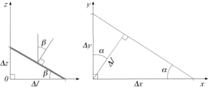
Fig. 1.Left: Vertical section in the steepest direction of the sloping surface. The grey line indicates the surface. Right: Projection of the sloping surface into the horizontalx−yplane atz=0.
Munk (1954a, b). Recently Munk has pointed out several problems related to the roughness of the sea (Munk, 2009). A detailed discussion together with further references can be found in Walker (1994).
We will apply the notation of Cox and Munk (1954a, b) whenever practical. Letx designate the crosswind coordi-nate,ythe upwind coordinate, andzthe elevation of the sur-face, wherez=0 describes the ocean at rest. Assume that a part of the surface is inclined relative to the horizontal sur-face, and let this part have an area vector of unit length at right angles to the area. This vector makes an angleβ with the z axis (Fig. 1), andβ is also the angle between the sur-face and the horizontal plane z=0. The projection of the area vector into thex−yplane has an azimuth angleαwith they axis, whereαis positive to the right of the upwind di-rection (Fig. 1). The didi-rection of the projected area vector is then the direction where the slope is steepest. The slope of the inclined surface becomesm=tanβ. Let1lbe the pro-jection of the area vector into thex−yplane (Fig. 1) and1z a height on thezaxis, related tomand1lby
1z
1l =m=tanβ. (1)
A line normal to1lintersects thex andy axes at the two points
1x=1l/sinα , 1y=1l/cosα. (2) The slopes of the surface in thex andy directions can be written by combining Eqs. (1) and (2)
zx=
∂z
∂x= 1z
1x= 1z
1lsinα=msinα , (3) zy=
∂z ∂y=
1z 1y=
1z
1lcosα=mcosα.
Evidently the sum of the two squared slopesz2x andz2y be-comes
z2x+z2y=m2sin2α+cos2α=m2. (4) The mean values of the slopes in this equation can be written
z2
whereσc2andσu2are the mean square slopes in the crosswind (x)and upwind (y)directions, andσ2the mean square slope. Cox and Munk found from observations of sun glitter that the statistical distribution of slopes in the x and y direc-tions almost followed a two-dimensional Gaussian probabil-ity function. Their complete mathematical description can be simplified to a more approximate expression, and the distri-bution then becomes the Gaussian function
p(zx, zy)≈ 1 2π σcσu
exp
"
− z
2
x 2σ2
c
− z
2
y 2σ2
u
#
. (6)
The slopeszx andzyhave positive and negative values, and their mean values are zero. The double integral ofpdzx,dzy between−∞and +∞along both horizontal axes is equal to 1.
In the data set obtained by Cox and Munk the ratioσc2/σu2
varied in the range 0.54–1.0 with a mean value of 0.75. The mean square slopes were linear functions of the wind speed
W:
σc2=0.003+0.00192W, (7)
σu2=0.000+0.00316W, (8)
whereW is the wind speed in m s−1. The mean square slope
σ2was observed to be
σ2=σc2+σu2=0.003+0.00512W. (9) The light reflected toward the zenith arrives from all az-imuthal directions, and the measurements of radiance from the surface of the sea are taken for different azimuthal direc-tions of the Sun. The probability distribution of the slopes has therefore been simplified to the one-dimensional case
p(m)=dN dm≈
1
(2π )0.5σ exp "
−m
2
2σ2 #
, (10)
wheredN is the fractional number of slopes of valuemper slope unitdm. If we introduce the normalized slope
s=m/σ, (11)
the Gauss function obtains the form
p(s)=dN ds ≈
1
(2π )0.5exp " −s 2 2 # . (12)
The integral of pds=dN for s between−∞ and +∞ is equal to 1. The cumulated probability of the normalized slope being in the interval from -∞tosis expressed by
P (s)=
s
Z
−∞
p(s′)ds′=
s
Z
−∞ 1
(2π )0.5exp "
−s
′2
2
#
ds′, (13)
and according to Abramowitz and Stegun (1970, eq. 26.2.17)
P (s)can be approximated by
P (s)≈1−p(s)hb1t+b2t2+b3t3+b4t4+b5t5 i
(14)
wheret= 1
1+0.2316419s
b1=0.319381530;b2= −0.356563782;b3=1.781477937; b4= −1.821255978; b5=1.330274429; with an error <
10−7.
A radiance from the zenith angleθ has an angle of inci-dence i at the surface and an angle of reflection r, where
i=r. If the radiance is reflected towards zenith, then the sumi+r is equal toθ, orθ/2=i=r. Moreover, the slope of the surface producing this reflection must have a slope angle β=i=r=θ/2, as shown by Fig. 2. This means that slopes reflecting radiance towards zenith cannot be steeper thanβ=45◦, and thatsin our case is related toθby
s=m σ =
tanβ
σ =
tan(θ/2)
σ . (15)
The cumulative probability distribution forsbeing in the in-terval from−stosis expressed byP (s)−P (−s). This dis-tribution is presented in Fig. 3 for the wind speeds 0, 2, 5 and 10 m s−1. Rather than usingsas the variable along the horizontal axis, the related zenith angle θ of Eq. (15) has been applied. We see that 90% of the slopes reflecting radi-ance towards zenith corresponds approximately to directions ofθ≤10◦, 20◦, 30◦and 40◦for the increasing wind speeds. That is, the higher the wind speed, the more parts of the sky contribute to the reflected radiance towards the zenith.
The upward radiance below the surface that is refracted and transmitted through the sloping surface towards zenith as the water-leaving radiance must have an anglej in water, relative to the normal to the surface, so that the correspond-ing refracted ray in air obtains the angleβ=rrelative to the normal to the surface (Fig. 2). The relationship betweenj
andβis expressed by Snell’s Law:
sinβ=sinr=nsinj, (16)
wherenis the refractive index of sea water. Fig. 2 shows that the zenith-directed radiance in air has a nadir angle in water,
θw, related toβandjby
θw=β−j=β−arcsin
sinβ n
. (17)
The corresponding cumulative distribution functionP (s)− P (−s) is shown in Fig. 4 for the wind speeds 0, 2, 5 and 10 m s−1, as a function of the nadir angle in water,θw. This
θ
β
θ
Fig. 2.Vertical section in the steepest direction of the sloping sur-face, indicated by the grey line. A ray from the zenith angleθin the sky has an angle of incidenceiand is reflected towards zenith in an angle of reflectionr equal toiand slope angleβ. A ray from the nadir angleθwin the sea has an angle of incidencejand is refracted
through the surface at an angle of refractionr with a direction to-wards zenith.
2.2 Calculation of reflected sky radiance and sun glitter at the foam-free surface
For the present study it is useful to separate the reflected radi-anceLrinto the part consisting of reflected radiance from the
sky,Lr,sky, the part consisting of reflected solar rays, termed
the sun glitter,Lr,sun, and the part consisting of reflected
ra-diance from both sky and sun,Lr,foam, reflected at the
foam-covered parts of the surface. We will start by discussing the two first terms, since these are both functions of the slope distribution. Azimuthal mean valuesLof the sky radiance have been used since the slopes contributing to the reflected radiance are supposed to be oriented at random. The mean radiances were originally observed for the zenith angles 0◦– 15◦–30◦–45◦–60◦–75◦by Høkedal and Aas (1998) and pre-sented in tables.
From these tabulated values the mean radiances for each degree in the intervals have been interpolated, and in the range θ=75◦–90◦ it has been assumed that the radiance is equal toL(75◦). Then the mean values ofLfor theθ inter-vals 0◦–1◦, 1◦–2◦, 2◦–3◦, ...89◦–90◦have been calculated. A small increase ofθ by1θ=1◦corresponds to an increase of
β by1β=0.5◦. Consequently the seriesθ=0◦, 1◦, 2◦,...90◦ has a series of reflecting surfaces with anglesβ=0◦, 0.5◦, 1◦,
θ Fig. 3. The cumulative probabilityP (s)−P(−s) as a function of the zenith angleθ in air corresponding tos. The curves represent from top to bottom the wind speeds 0, 2, 5 and 10 m s−1.
θ Fig. 4. The cumulative probabilityP (s)−P (−s) as a function of the nadir angleθwin water corresponding tos. The curves represent from top to bottom the wind speeds 0, 2, 5 and 10 m s−1.
1.5◦,...45◦. This produces a series of mby Eq. (1) and for a fixed wind speed a series ofs by Eq. (11). The values of
P (s)have then been calculated for this series ofs values. The probability1Pthatsshould be in the interval fromsn−1
tosnis obtained by the subtraction
1P=P (sn)−P (sn−1). (18)
Thus for each intervalθ±1 θ/2 there is a slopesthat is able to reflect the radianceL(θ) towards the zenith, and1Pis the weighting function for the radiance fromθ. Instead of taking into account the negative values ofs, only the positive values between 0 and∞have been used, and accordingly1Phas been multiplied by 2. The sum of reflected sky radiances towards the zenith is therefore
Lr,sky= X
the air-water interface for an angle of incidence equal toθ/2. The problem of polarization will be discussed in Sect. 3.1.
As a test it has been confirmed that
X
(21P )=1. (20)
Since we are studying the radiance reflected towards the zenith, the azimuth angle between this direction and the po-sition of the sun is undetermined. The tabulated values of the irradianceEsun0 of the direct solar rays on a plane normal
to the rays (Høkedal and Aas, 1998) have accordingly been converted to equivalent azimuthal mean values of solar radi-ance. The angle of the solar diameter is approximately 0.5◦, but since our calculations apply1θ=1◦, it is practical to dis-tribute the solar radiation within the solid angle 2π sin(θs)
1θ=0.10966 sin(θs), whereθs is the solar zenith angle. The resulting equivalent solar radiance becomes
Lsun(θs)=Esun0/(0.1097 sinθs). (21) The average contribution from the sun glitter can then be de-scribed by an expression similar to Eq. (19):
Lr,sun=Lsun(θs)(21P )ρa,w(θs/2). (22) It should be emphasized that the values of the probability distribution functionP used in Eq. (19) and (22) is a sim-plified form of the Cox-Munk model, and that the average relationship between wind speed and mean square slopes, Eq. (9), is based on observations from the Hawaiian area of the Pacific Ocean. The corresponding relationship in Nordic coastal areas may be different due to differences in wind du-ration, fetch and boundary layer stabilities in the sea and at-mosphere. The coastline and bottom topography may also influence the sea state. Thus the results discussed here are only meant as a first approximation to the real local condi-tions.
2.3 Calculation of radiance reflected from the foam-covered part of the surface
It can easily be observed that the fraction F of the sur-face that is covered by foam and whitecaps from breaking waves increases with increasing wind speedW. The rela-tionship betweenF andWhas been discussed in several pa-pers, e.g. Monahan (1971), Monahan and O’Muircheartaigh (1980, 1981, 1986), and Wu (1979). Monahan and O’Muircheartaigh (1980) obtained by the method of least squares the power-law
F=2.95×10⁻⁶W3.52, (23) where W is in units of m s−1. The equation yields F =
0.0098 forW=10 m s−1. Thus less than 1% of the surface is covered by foam at wind speeds up to 10 m s−1. In a later work Monahan and O’Muircheartaigh (1986) estimatedF as a function of the temperature difference 1T =Tair−Tsea.
Using monthly mean values of1T for the Færder Light-house at the northern border of the Skagerrak, the values of
F become smaller than those obtained from Eq. (23). In the present study Eq. (23) is applied due to its simplicity.
Lauscher (1955) mentioned that foam of a sufficient thick-ness would reflect 50–80%. Whitlock et al. (1982) recorded the irradiance reflectanceρf0 of foam in a laboratory tank
and found that a reasonable constant value for the reflectance in the visible part of the spectrum at wavelengths of 440 nm and longer was ρf0=0.5±0.1. Also Frouin et al. (1996)
obtained values ofρf0 within the same range for breaking
waves in the surf zone at La Jolla, California. In the open sea the foam reflectance seems to be smaller than in these inves-tigations. Based on several series of photos from a research platform in the German Bight Koepke (1984) found that the time-averaged reflectance of the foam wasρf0=0.22±0.11
for wind speeds up to 10 m s−1.
It is well established that the reflection from foam in the near infrared is smaller than in the visible part (Whitlock et al., 1982; Frouin et al., 1996; Moore et al., 1998, 2000; Nico-las et al., 2001; Kokhanovsky, 2004). The spectral varia-tion in the visible part of the spectrum may depend on the thickness of the foam, according to Moore et al. (1998), who found that average reflectances at 410, 440, 510, 550, 670 and 860 nm were in the ranges 0.81–0.86, 1, 0.99–1.01, 0.98–0.99, 0.73–0.87, 0.38-0.59, respectively, when normal-ized at 440 nm. However, in a later work by the same au-thors (Moore et al., 2000) the reflectances seem to be con-stant from 410 to 670 nm, and then smaller at 860 nm. In this paperρf0has been given the constant value 0.22 for the
spectral range 405–650 nm. Visual observations of the foam in the Oslofjord-Skagerrak area, with its yellow substance-rich Case 2 waters, have indicated no spectral dependency.
Neglecting any bi-directional effects and assuming that the foam acts as a Lambertian emitter,ρf0can be related to the
upward reflected radiance from the patch or streak of foam,
Lr,foam,0, and the total downward irradiance in air,Etot, by ρf0=π Lr,foam,0/Etot. (24)
The foam-reflected radiance can then be written
Lr,foam,0= ρf0
π Etot. (25)
This radiance has to be weighted by the fractional areaF of the foam in order to obtain the average contributionLr,foam
to the total reflected radiance at the surface:
Lr,foam=F Lr,foam,0=F ρf0
π Etot. (26)
If F can be expressed by Eq. (23) and ρf0=0.22, then
Eq. (26) can be written
Lr,foam=F ρf0
π Etot=(2.07×10
−7W3.52)E
tot. (27)
Their augmented reflectance due to whitecaps and foam, 3.4×10⁻⁶W2.55, is close to the product Fρ
f0=0.65×
10−6W3.52 of Eq. (27) up to a wind speed of 7 m s−1, but
at stronger winds their reflectances are smaller. 2.4 Total reflected radiance at the surface
The total radiance reflected towards zenith at the surface of the sea can be written
Lr=(1−F )(Lr,sky+Lr,sun)+F Lr,foam,0, (28)
where the radiances have been weighted by their respective fractions of surface area. However, sinceF ≤1% according to Eq. (23) whenW≤10 m s−1, Eq. (28) may without any significant loss of accuracy be simplified to
Lr=Lr,sky+Lr,sun+F Lr,foam,0=Lr,sky+Lr,sun+Lr,foam. (29)
Lr,foam is directly related toEtot by Eq. (27), andLr,sun is
related toEsun by Eqs. (21–22). Etot can be separated into
the contributions from the diffuse sky irradianceEskyand the
direct solar irradianceEsun
Etot=Esky+Esun. (30)
Lr,skyandEskyare both functions of the azimuthal mean
val-uesL(θ) of the sky radiance; Lr,sky by Eq. (19), andEsky
by
Esky=2π
π/2
Z
0
L(θ )sin(θ )cos(θ )dθ=π
π/2
Z
0
L(θ )sin(2θ )dθ . (31)
All three terms of the reflected radianceLrcan then by
cal-culated, providedL(θ), Esun,0 or Esun, and W have been
recorded.
2.5 Calculation of water-leaving radiance
From the definition of radiance and Snell’s Law it can readily be obtained that an upward radiance just beneath the surface,
L0w−, produces a contribution1Lwto the water-leaving
radi-ance by
1Lw=L0w− τ
n2, (32)
whereτ is the transmittance of radiance through the water-air interface. The azimuthal mean value of L0−
w from the
nadir angleθwis denoted L0w−(θw). Assume that we know
this mean value for all theθw intervals 0◦–1◦, 1◦–2◦, 2◦–
3◦, ...89◦–90◦. This series ofθw intervals corresponds to a
series ofβ intervals determined by Eqs. (16–17). Note that although1θwis constant,1β decreases with increasingθw
due to Snell’s Law. The new series ofβintervals produces a series ofmby Eq. (1) and for a fixed wind speed a series ofs
intervals by Eq. (11). For eachsinterval there is a probability
1Pforsbeing in this interval (Eq. 18).
The total water-leaving radiance is the sum of the contribu-tions from all upward radiances in water, transmitted through the surface and refracted towards zenith:
Lw= X
L0w−(θw)(21P ) τ (j )
n2 . (33)
The sum is for all the θw intervals 0◦–1◦, 1◦–2◦, 2◦–3◦,
...89◦–90◦, andτ(j )is the Fresnel transmittance at the water-air interface for an angle of incidence equal toj.
2.6 Observations of radiance and irradiance from sky and sun
A total of 52 data sets of angular distributions of sky radiance and direct solar irradiances, representing 9 different days with a clear sky, were collected in Oslo by Høkedal and Aas (1998) at the wavelengths 405, 450, 520, 550 and 650 nm, for solar zenith angles in the range 37◦–76◦. The record-ings were made manually by means of a tripod and a rotating Gershun tube provided with interference filters, often located on the roof of the high department building at the University of Oslo. The Gershun tube was of local construction (Aas, 1993), and its opening half-angle was 5.5◦in order to ensure stable signals. Details of the calibration have been presented elsewhere (Aas, 1993). Measurements were taken over the upper hemisphere in steps of 1θ=15◦ (range 0◦–75◦) and
1α=24–36◦(range 0◦–180◦). The time required for a com-plete recording with one filter was 15–20 min. During that time the solar zenith angleθs would have changed by 0◦at noon, and 3◦in the afternoon, implying that the atmospheric conditions could be regarded as practically constant for our purposes. A full spectral series took 80–90 min, correspond-ing to1θs=7◦–15◦. The radianceL(θ,α) and the solar irradi-anceEsunwere recorded directly by the Gershun tube, while Eskywas obtained by integration ofL(θ,α) (Eq. 31), andEtot
was then found by using Eq. (30). An earlier analysis of the results has been presented by Aas and Høkedal (1999). 2.7 Observations of sub-surface radiance and
irradiance
During the Nordic Cruise to the Mediterranean in 1971 an extensive set of radiance and polarization data was collected onboard the R/V Helland-Hansen by Lundgren with an in-strument constructed by the same person (Lundgren, 1971). The radiance sensor had an opening half-angle of 0.7◦, and the wavelengths were in the range 405–502 nm. The sub-surface radiance field was recorded in steps of1θw=5◦–30◦,
Observations of radiance from nadir and upward and downward irradiance in the Oslofjord and Skagerrak, to-gether with downward irradiance above the surface, have been collected by the Norwegian Institute for Water Re-search and the University of Oslo during several co-projects. The measurements have usually been taken onboard the R/V Trygve Braarud and G. M. Dannevig with the PRR-600 from Biospherical Instruments, San Diego, California, and the deck reference has been the PRR-601. The wavelengths are 412, 443, 490, 510, 555 and 665 nm, and the opening half-angle of the radiance sensor is 10◦ in water. The immer-sion coefficients provided by the manufacturer have been ap-plied, and the self-shading effect (Gordon and Ding, 1992; Zibordi and Ferrari, 1995; Aas and Korsbø, 1997) has been accounted for. The upward radiance just beneath the surface,
L0−
w , was obtained by upward extrapolation from a depth of
0.5–1 m. This method requires that the vertical attenuation coefficient of the radiance is approximately constant within the upper meters of the surface layer. Factors like wave ac-tion, bubbles and accumulation of phytoplankton and detritus close to the surface may destroy the assumed constancy and thus influence the accuracy of the estimatedL0w−, but as ex-plained in another work (Aas et al., 2009), no clear signs of such influences have ever been found in the vertical profiles.
3 Results and discussion
3.1 Lr,skyLr,sunandLr,foam
The observations of sky radiance made by Høkedal and Aas (1998) did not include the degree of polarization, except on two dates, and the reflectances were therefore calculated as if the radiance from the sky was unpolarized. This is cer-tainly not correct. Their analyses showed that by neglecting the polarization the relative error of the reflected radiance for a flat sea might range from−39% to +14%. A negative error means that the calculated reflectance is less than the correct value. The reflected sky irradiance, based on radiances from the whole hemisphere, was underestimated by 2% to 5%. In the present analysis azimuthal mean values of the radiances are used, and a further analysis of the measurements shows that the relative errors of the corresponding reflectances are in the range from−10% to +1% for radiances incident from zenith angles between 15◦ and 75◦. If only zenith angles up to 45◦ are taken into account, then the range of the rel-ative errors will be reduced, extending from−4% to +1% with a mean value of−2%. The slope distribution function
1P(Eq. 18) gives more weight to the smaller values of θ
than to the larger ones, as demonstrated by Fig. 5, and the polarization errors are smaller for the smaller values ofθ. Figure 3, as already mentioned, shows that 90% of the con-tribution to the reflected radiance towards zenith comes from zenith angles less than 40◦for wind speeds up to 10 m s−1. Thus it seems reasonable to assume that on average our
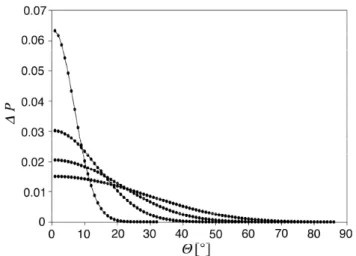
cal-Δ θ
Fig. 5. The probability distribution1P as a function of the cor-responding zenith angleθin air. The curves represent from top to bottom in the left part of the graph the wind speeds 0, 2, 5 and 10 m s−1.
culated reflectances may be underestimated by 2% due to the neglected polarization.
Kattawar and Adams (1990) used Monte Carlo simula-tions to study the effect of polarization on reflected and trans-mitted radiance at the surface of the sea. They found that errors up to 30% might occur in the radiances if the polar-ization was neglected. On the other hand, their results also showed that a positive error for one azimuth direction tended to be partly compensated for by a negative error for the oppo-site direction. The resulting errors of the azimuthal mean val-ues of the radiances can be read off as ranging from 0 to 9%. Kattawar and Adams also found that the error of neglecting polarization effects in the calculation of irradiance reflected upwards at the surface was≤2%. Consequently their model results support the field results of Høkedal and Aas.
Two factors influencing the amount of reflected light, espe-cially for directions of incidence close to the horizon, are the processes of shadowing and multiple reflections. A facet of the surface may experience shadowing from other parts of the wave and from other waves, thus reducing the amount of re-flected light. The process of multiple reflections, on the other hand, increases the reflectance for some directions. The in-fluence of these effects on the upward-reflected light from the sea surface has been discussed by Preisendorfer and Mobley (1986) and Gordon and Wang (1992a, b). In the present pa-per the effects have not been taken into account, since more than 90% of the contributions to the zenith-reflected light comes from zenith angles less than 40◦for wind speeds up to 10 m s−1, that is from directions closer to the zenith than to the horizon.
The 52 data sets described in Sect. 2.6 were used to cal-culateLr,sky, Lr,sun andLr,foam, as expressed by Eqs. (19,
22) and (27), andLrwas then obtained by adding the three
θ
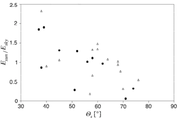
Fig. 6. The ratioEsun/Eskyas a function of the solar zenith angle θs.The filled circles and open triangles represent 405 and 650 nm,
respectively. The ratios are normalized against their mean values at these wavelengths.
for a refractive index of 1.340, corresponding to the aver-age conditions of salinity, temperature and wavelength being approximately 30, 15◦C and 550 nm, respectively. The vari-ation of the reflectances with regard to these three parameters is insignificant compared to the mentioned uncertainty intro-duced by the polarization.
3.2 The ratioLr/L(0◦)
The obvious method (e.g. Austin, 1974) to estimateLr for
a flat sea and a certain direction of observation 180◦–θis to record the sky radiance in the same plane of incidence but from the zenith angleθ, and multiply the radiance by the corresponding Fresnel reflectanceρa,w. In our case, whereθ is 0◦, the radiance reflected at the surface towards the zenith could be written
Lr=L(0◦)ρa,w(0◦), (34)
The ratioLr/L(0◦) is
Lr/L(0◦)=ρa,w(0◦)=0.0211, (35) where ρa,w(0◦)=0.0211 is the value of the Fresnel re-flectance used in our calculations for a ray of normal inci-dence. However, for a surface roughened by the wind the reflectanceρa,wwill depend on the wind speed and the solar zenith angle, and because our case with zenith-reflected ra-diance is outside the recommended range of viewing angles (references in Sect. 1), we must expect significant contribu-tions from direct solar glitter.
The results for the ratioLr/L(0◦), calculated by Eqs. (19,
22, 27, 29), and presented in Table 1, show that the flat-sea estimate ofLr/L(0◦) expressed by Eq. (35) works well for a
zero wind speed, since the ratio is within the range 0.0201– 0.0220, with a mean value of 0.0215. The small deviations from a constant value are due to the mean square slope which
is not zero even in the absence of wind, but 0.003 according to Eq. (9). When the wind speedW increases up to 10 m s−1,
the mean value of the ratio increases from 0.0215 to 0.0784, which is a factor 3.7 greater than the value 0.0211 suggested by Eq. (35). In one case the ratio becomes 0.388, which is greater than 0.0211 by a factor of 18. The mean value ofθs in Table 1 is 58◦, and it is noteworthy that the simulations of Mobley (1999, Fig. 6) forW=10 m s−1and a nadir viewing angle seem to produce a mean value of the ratio of approxi-mately 0.03 for the same solar zenith angle. This is less than half of the present result. Mobley points out the importance of the input from the sky radiance distribution, and it is pos-sible that the difference in results may be due to different inputs.
If we separateLr/L(0◦) into the componentsLr,sky/L(0◦), Lr,sun/L(0◦) andLr,foam/L(0◦), we find thatLr,sky/L(0◦) only
ranges from 0.020 to 0.029 (Table 1). It also becomes clear thatLr,sun/L(0◦) represents the smallest and greatest
normal-ized reflectances toward the zenith (Table 1), ranging from 0 to 0.31. An interesting result is that the ratioLr,sun/L(0◦)
is much smaller thanLr,sky/L(0◦) for certain values ofθs, as listed by Table 2. In these cases the contribution from sun glitter to the radiance directed towards the zenith can be neglected. Table 1 shows that the radiance reflected from foam can be neglected at a wind speed of W=5 m s−1, but contributes significantly to Lr (24% on an average) when W=10 m s−1. A closer examination of the data reveals that
Lr,foam/L(0◦) reaches the value of 0.001 at wind speeds
be-tween 5 and 7 m s−1, implying thatLr,foam should be taken
into account whenever the wind speed is greater than 5 m s−1.
This is consistent with the sea state described by the Beau-fort wind scale (Sect. 1). The ratio Lr,foam/Lr,sky tends to
decrease with increasingθs.
The results of Table 2 indicate that in the Northern Skager-rak, where the solar zenith anglesθs≥37◦, Eq. (35) is only valid when the wind speed is low (W <2 m s−1). At higher wind speeds (W >2 m s−1), Eq. (35) is valid for a restricted range ofθs, where the lower limit of the range increases with increasing wind speed. When the wind speed is 10 m s−1,θs should be approximately 80◦or greater in order to avoid sun glitter in the zenith direction. Table 2 also implies that in the Polar regions, where the sun is low, solar glitter is probably not a problem at moderate wind speeds when the direction of observation is close to the nadir.
Rather than using the constant Fresnel reflectance 0.0211 to represent the ratioLr/L(0◦) in Eq. (35), we could
approxi-mate the ratiosLr,sky/L(0◦),Lr,sun/L(0◦) andLr,foam/L(0◦)
by their respective bulk mean spectral values for all solar zenith angles in the present data set, and test if that im-proved the results. Table 3 shows that the standard devia-tion from the mean value of Lr,sky/L(0◦) is now less than
0.002 at wavelengths 405, 450, 520, 550 and 650 nm, and for wind speeds up to 10 m s−1. The maximum deviation of
Lr,sky/L(0◦) from the mean value in the obtained data set is
Table 1.Statistical properties of radiance ratios. Deviations are from the mean value.
Lr/L(0◦) Lr,sky/L(0◦) Lr,sun/L(0◦) Lr,foam/L(0◦)
W[m s−1] 0 5 10 0 5 10 0 5 10 0 5 10
Mean value 0.0215 0.0348 0.0784 0.0215 0.0237 0.0260 0 0.0110 0.0333 0 0.0002 0.0191 Minimum value 0.0201 0.0232 0.0298 0.0201 0.0198 0.0206 0 0 0.0002 0 0.0000 0.0040 Maximum value 0.0220 0.1901 0.3884 0.0220 0.0253 0.0292 0 0.1672 0.3145 0 0.0005 0.0531 Standard deviation 0.0003 0.0261 0.0575 0.0003 0.0010 0.0018 0 0.0264 0.0494 0 0.0001 0.0137 Max. deviation 0.0014 0.1553 0.3100 0.0014 0.0039 0.0055 0 0.1563 0.2813 0 0.0003 0.0339
Table 2.Ranges ofθswhere sun glitter can be neglected.
W[m s−1] Lr,sun/L(0
◦)<0.002 L
r,sun/L(0◦)<0.001
θs θs
0 ≥37◦ ≥37◦
1 ≥37◦ ≥37◦
2 ≥47◦ ≥50◦
3 ≥55◦ ≥57◦
5 ≥65◦ ≥68◦
10 ≥78◦
much smaller thanLr,sky/L(0◦), were not used in the
statis-tical calculations ofLr,sun/L(0◦). Unfortunately the standard
and maximum deviations for this ratio are still too great to be acceptable, amounting to 0.24 in the red part of the spec-trum forW=10 m s−1. The deviations ofLr,foam/L(0◦) from
the mean values at the different wavelengths are of the same order of magnitude asLr,sky/L(0◦) whenW=10 m s−1.
Ac-cordingly the use of the bulk mean value to estimate the ratios
Lr,sun/L(0◦) andLr,foam/L(0◦) is not a satisfactory method.
An additional experiment has been conducted by ap-proximating the three ratios Lr,sky/L(0◦), Lr,sun/L(0◦) and Lr,foam/L(0◦) by best-fit second order polynomials on the
formA+B1θs+B2θs2, whereA,B1andB2are constants,
for the different wavelengths and wind speeds. The errors are then reduced, but they are still too large forLr,sun/L(0◦)
andLr,foam/L(0◦). At winds of 5 and 10 m s−1 the errors
of Lr,sun/L(0◦) amounted to 0.025 and 0.047, respectively,
and at 10 m s−1the errors ofL
r,foam/L(0◦) could reach 0.013.
These errors are of the same order of magnitude as the mean values ofLr,sky/L(0◦), 0.022–0.026, as shown by Table 1.
The ratioLr,sky/L(0◦) can be described with satisfactory
accuracy by the mean values of Tables 1 and 3, and by the second order polynomials ofθs in Table 5. An additional useful property of the ratio is that if the value ofLr,sky/L(0◦)
is known at one wavelength, then this value can be applied to the other wavelengths as well. For instance, if the ratio is known at 405 nm, then the assumption that the ratio is the same at the other wavelengths, leads to relative RMS errors of 1–4–7% for the wind speeds 0–5–10 m s−1, respectively.
These errors are rather small compared to other errors con-nected with field measurements.
The “dark pixel” assumption is that in the near infrared the total radiance from the sea will mainly consist of sky and solar radiance reflected at the surface. If our zenith-reflected radiance contains no sun glints, then the ratio Lr,sky/L(0◦)
can be assumed constant with wavelength and equal to the recorded value ofLr/L(0◦) in the near infrared (Morel 1980).
The different tests discussed here demonstrate that while the reflected sky radianceLr,skyis normalized in a useful way
by the sky radianceL(0◦), this normalization does not work for the sun glitterLr,sunand the foam-reflectedLr,foam.
Con-sequently better normalizing quantities or reference inputs should be found for these two radiances. It was pointed out in Sect. 2.4 howLr,foamis related toEtot, andLr,suntoEsun.
It was also mentioned thatLr,skyis indirectly related toEsky,
since both quantities are functions of the sky radianceL(θ). A common normalizing quantity is unrealistic because there is no constant ratio betweenEskyandEsunat a given
wave-length, wind speed or solar zenith angel. The ratio varies in an unpredictable way due to different optical conditions of the atmosphere, as displayed by Fig. 6. HereEsun/Eskyvaries
by an order of magnitude, both in the violet (405 nm) and red (650 nm) parts of the spectrum. During the measurements of the two irradiances the solar zenith angle only varied by 0◦– 3◦, and the varying values ofE
sun/Eskyshown by Fig. 6 must
accordingly be due to variation of the atmospheric conditions from one day to another.
3.3 The ratiosLr,foam/Etot,Lr,sun/EsunandLr,sky/Esky
At a given wind speedLr,foamis a linear function ofEtot, as
shown by Eq. (27). The constant of proportionality is inde-pendent of the wavelength and solar angle, and depends only on the wind speed by a power-law.
The sun glitterLr,sunis related to Esun by Eqs. (21–22),
Table 3.Statistical properties of radiance ratios at different wavelengths.
Wavelength [nm] W[m s−1]
Lr,sky/L(0◦) Lr,sun/L(0◦) Lr,foam/L(0◦)
allθs θs=37◦–60◦ θs=37◦–70◦ allθs
0 5 10 5 10 10
405
Mean value 0.0213 0.0228 0.0243 0.0102 0.0216 0.0079 Standard deviation 0.0004 0.0011 0.0016 0.0119 0.0189 0.0024 Max. deviation 0.0012 0.0030 0.0037 0.0215 0.0350 0.0039
450
Mean value 0.0215 0.0234 0.0254 0.0094 0.0215 0.0106 Standard deviation 0.0001 0.0005 0.0011 0.0124 0.0203 0.0038 Max. deviation 0.0002 0.0008 0.0021 0.0227 0.0459 0.0059
520
Mean value 0.0215 0.0239 0.0262 0.0185 0.0419 0.0162 Standard deviation 0.0003 0.0006 0.0008 0.0293 0.0467 0.0071 Max. deviation 0.0007 0.0014 0.0013 0.0572 0.1005 0.0101
550
Mean value 0.0216 0.0241 0.0270 0.0093 0.0306 0.0214 Standard deviation 0.0002 0.0008 0.0016 0.0121 0.0200 0.0101 Max. deviation 0.0005 0.0018 0.0038 0.0214 0.0305 0.0158
650
Mean value 0.0216 0.0242 0.0272 0.0381 0.0730 0.0368 Standard deviation 0.0004 0.0012 0.0021 0.0592 0.0860 0.0138 Max. deviation 0.0009 0.0028 0.0050 0.1292 0.2415 0.0264
Table 4. Relative RMS error of estimates in % by two different normalizations.
Wavelength Lr,sun/L(0◦) Lr,sun/Esun
[nm] W=5 m s−1 W=10 m s−1 W=5 m s−1 W=10 m s−1
405 70 69 12 8
450 246 113 5 6
520 148 140 12 4
550 185 118 8 12
650 387 128 21 4
best-fit polynomials on the formA+B1θs+B2θ2s. We now find that the results are much more coherent than when the normalization was made byL(0◦), as can clearly be seen by comparing the results in Table 4. The striking fit between the polynomials andLr,sun/Esun is shown by Fig. 7. The
poly-nomials for sun glitter reflected in the zenith direction at the wind speeds 3, 5 and 10 m s−1are presented in Table 5. An interesting and useful property ofLr,sun/Esunis that its value
is independent of wavelength, so that if its value is known at one wavelength, then the value is also known at all other wavelengths. This was pointed out by Zibordi et al. (2002), and the constancy is due to the very small spectral variation of the refractive index of sea water.
SimilarlyLr,skyhas been normalized byEskyin order to
see whether the earlier results forLr,sky/L(0◦) can be
im-proved. However, whenLr,sky/Eskyis approximated by
best-fit polynomials ofθs, the overall errors of the resultingLr,sky
are slightly greater than whenLr,sky/L(0◦) was estimated in
θ
Fig. 7.The ratioLr,sun/Esunas a function ofθs, at the wavelengths
405, 450, 520, 550 and 650 nm. Only ratios greater than 0.0001 are taken into account. The best-fit lines represent, from bottom to top, the wind speeds 3, 5 and 10 m s−1, and their polynomials are presented in Table 5.
the same way. This is not surprising, since the sky radiances contributing to Lr,sky have directions and values closer to L(0◦) than the radiances from the whole hemisphere con-tributing toEsky. Consequently, ifL(0◦) has been observed,
the overall best estimates ofLr,skywill be obtained by using
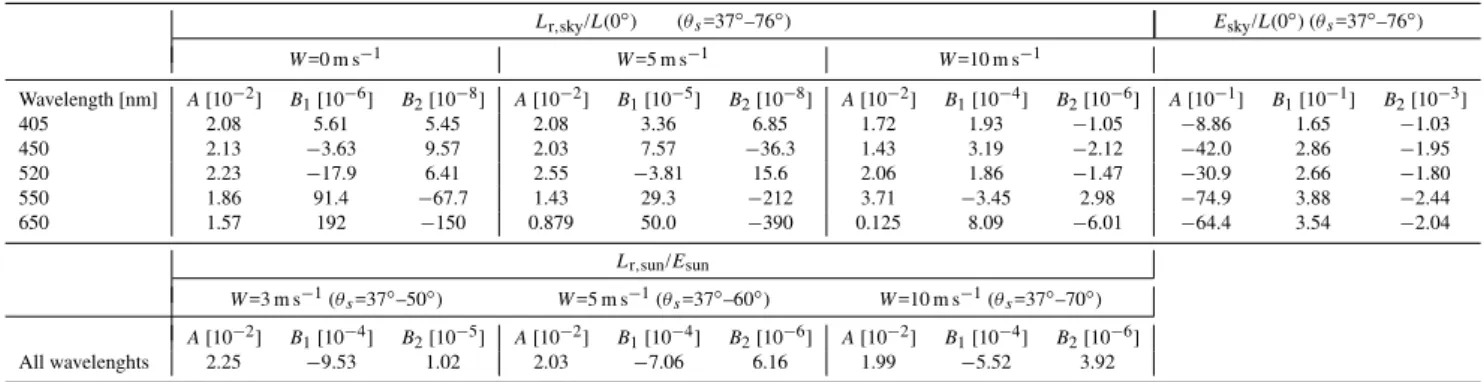
Table 5.Polynomials forLr,sky/L(0◦),Lr,sun/Esun, andEsky/L(0◦) on the formA+B1θs+B2θs2, whereθsis in units of degrees.
Lr,sky/L(0◦) (θ
s=37◦–76◦) Esky/L(0◦) (θs=37◦–76◦)
W=0 m s−1 W=5 m s−1 W=10 m s−1
Wavelength [nm] A[10−2] B1[10−6] B2[10−8] A[10−2] B1[10−5] B2[10−8] A[10−2] B1[10−4] B2[10−6] A[10−1] B1[10−1] B2[10−3]
405 2.08 5.61 5.45 2.08 3.36 6.85 1.72 1.93 −1.05 −8.86 1.65 −1.03
450 2.13 −3.63 9.57 2.03 7.57 −36.3 1.43 3.19 −2.12 −42.0 2.86 −1.95
520 2.23 −17.9 6.41 2.55 −3.81 15.6 2.06 1.86 −1.47 −30.9 2.66 −1.80
550 1.86 91.4 −67.7 1.43 29.3 −212 3.71 −3.45 2.98 −74.9 3.88 −2.44
650 1.57 192 −150 0.879 50.0 −390 0.125 8.09 −6.01 −64.4 3.54 −2.04
Lr,sun/Esun
W=3 m s−1(θ
s=37◦–50◦) W=5 m s−1(θs=37◦–60◦) W=10 m s−1(θs=37◦–70◦)
A[10−2] B1[10−4] B2[10−5] A[10−2] B1[10−4] B2[10−6] A[10−2] B1[10−4] B2[10−6] All wavelenghts 2.25 −9.53 1.02 2.03 −7.06 6.16 1.99 −5.52 3.92
3.4 The ratioLr/Etot
If the downward solar irradianceEsunand the downward
ra-dianceL(0◦) have been observed, and the wind speedWand solar zenith angleθs are known, then it is possible to obtain estimates ofLr,skyandLr,sunby the polynomials in Table 5.
If, in addition,Etot has been observed,Lr,foam can be
esti-mated by Eq. (27). The total reflectanceLr as well as the
normalized total reflectanceLr/Etotare then determined.
There is one objection that can be raised if one intends to apply this procedure to automatic recordings at sea, namely the problem of observingEsun. WhileEtotandL(0◦) are
eas-ily measured by continuously recording sensors, the determi-nation ofEsunis not a routine operation. It can be recorded
manually by simple devices or automatically by high tech-nology instruments, but such instruments are not suitable for mounting on a ship where they are exposed to varying weather conditions. The movements of the ship represent an additional problem. Fortunately, sinceEskyis related to L(0◦) by a hemispherical integral includingL(0◦), it is pos-sible to estimate Esky from the observed L(0◦) with
satis-factory accuracy. The use of second order polynomials of
θsto approximate the ratioEsky/L(0◦) at the different
wave-lengths results in a relative RMS error of 6% for the esti-matedEsky. The polynomials forEsky/L(0◦) are presented
in Table 5. WhenEskyhas been estimated fromL(0◦) and θs,Esuncan be found by subtractingEskyfrom the observed Etot.
The polynomials of Table 5 and Eq. (27) can now be ap-plied to estimate the normalized reflectance towards zenith,
Lr/Etot. The complete procedure has been tested and
com-pared to the directly calculated values ofLr/Etot (Fig. 8).
The RMS value of the errors by using the polynomials is
≤0.0001 at all wind speeds≤10 m s−1, while the relative
er-rors are≤5%.
It may be pointed out that the influences of the solar zenith angle and the wavelength on the estimated ratioLr,sky/L(0◦)
are rather small in our case. If we approximate the values ofLr,sky/L(0◦) by the spectral mean values of Table 3 rather
Fig. 8. The ratioLr/Etot obtained from the polynomials of Ta-ble 5 as a function of the same ratio calculated from the radiance and slope distributions, at the wavelengths 405, 450, 520, 550 and 650 nm, and at the wind speeds 0, 5 and 10 m s−1.
than by the polynomials of Table 5, thus disregarding the so-lar zenith angle, the RMS value of the errors for the estimated total reflectanceLr/Etotwill increase only slightly, from 2.0–
6.7–8.1 to 2.3–7.0–10.6 in units of 10−5for the wind speeds 0–5–10 m s−1, respectively, and as we see the error will still be≤0.0001 at all wind speeds≤10 m s−1. If we also disre-gard the influence of wavelength on the ratioLr,sky/L(0◦) by
using the mean values ofLr,sky/L(0◦) from Table 1, the RMS
value of the estimatedLr/Etotremains practically the same
as in the last case.
In the present study the applied wavelengths have been 405, 450, 520, 550 and 650 nm. These wavelengths are different from the channels of the satellite sensors MERIS, MODIS and SeaWiFS. However, based on the spectral dis-tributions ofLr/Etotfound here, it seems that linear spectral
interpolation ofLr/Etotis a satisfactory method for
obtain-ing values at other wavelengths.
The results at different wind speeds have mostly been pre-sented for 0, 5 and 10 m s−1. Comparison with results at other wind speeds indicates thatLr/Etotmay be interpolated
as a linear function ofW. 3.5 The ratioLw/Lr
The azimuthal mean valuesL0w−(θw)of the sub-surface
radi-ance can be converted to the water-leaving radiradi-anceLw by
Eq. (32). It was observed in Sect. 2.1 that for wind speeds up to 10 m s−1, 90% of the directions contributing to L
w had
nadir angles θw in water less than 6◦. Within this small
angular interval L0−
w (θw) is practically constant. Tyler’s
(1960) observations of blue radiance in Lake Pend Oreille result in the value 1.03 for the ratio L0w−(10◦)/L0w−(0◦)
close to the surface. Based on linear interpolation the ratio
L0w−(5◦)/L0w−(0◦)should then have the value 1.015. Similar observations by Lundgren in the Mediterranean at a depth of 0.5–1 m (Aas et al., 1997) indicate values in a range from 1.00 to 1.01 forL0w−(10◦)/L0w−(0◦), and even closer to 1.00 forL0w−(5◦)/L0w−(0◦).
The data set of radiances and irradiances from the Oslofjord-Skagerrak area, described in Sect. 2.7, has been restricted to those 12 stations where 50 % of the sky or more was free of clouds, and whereθs was smaller than 76◦. Be-cause the instrument only records radiance from nadir, the radiance at other angles has to be estimated by other meth-ods, like for instance theαmodel (Aas and Højerslev, 1999). This model approximates the azimuthal averageLu(θw)of upward radiance by the function
Lu(θw)=Lu(0◦)
1+α
1+αcosθw
, (36)
whereθwis the nadir angle in water, andαis defined by α=Lu(90
◦)
Lu(0◦)
−1. (37)
TheQfactor is defined as the ratio between upward irradi-ance and nadir radiirradi-ance, and by integrating Eq. (36) over the lower hemisphere it is readily found that
Q=2π1+α
α2 [α−ln(1+α)]. (38)
Just beneath the surface Q exhibited values from 3.16 to 5.80, and by combining Eqs. (36–38), the esti-mates of L0w−(10◦)/Lw0−(0◦) become 1.01±0.01, and for
L0w−(5◦)/L0w−(0◦)the deviations from 1.00 are less than 0.01. Thus the Case 2 waters of the Lake Pend Oreille and the
Oslofjord-Skagerrak area, as well as the Case 1 waters of the Mediterranean, show thatL0−
w is practically constant for
all nadir angles equal to or less than 10◦.
It is therefore a reasonable approximation to make the sub-stitutionL0w−(θw)≈L0w−(0◦)in Eq. (33). The radiance
trans-mittanceτ(j )is 0.979 whenθwis in the small range from 0◦
to 10◦. By usingn=1.340, Eq. (33) can then be approximated by
Lw≈L0w−(0
◦
)0.979
1.3402 X
21P=0.545L0w−(0◦), (39) since the sum of all probabilities is 1 (Eq. 20). It should be noted that the ratioLw/L0w−(0◦)is a constant value,
indepen-dent of the wavelength and the wind speed. Aas et al. (2009) obtained the value 0.546 for this ratio by a different proce-dure, as an approximation for a flat sea.
The normalized water-leaving radiances Lw/Etot have
been calculated, and the results have been extrapolated and interpolated to the wavelengths used in this paper. The wind speed at the stations ranged from 1.5 to 7.5 m s−1, with an average value and standard deviation equal to 4 and 2 m s−1, respectively. For each station with a value ofLw/Etot the
atmospheric data that were closest with regard to θs were chosen, and the corresponding value ofLr/Etotwas then
cal-culated for the same wind speed. The ratio betweenLw/Etot
andLr/Etotmay then provide a tentative estimate ofLw/Lr.
The results are presented in Table 6, which shows that
Lw/Lrat the chosen stations on an average varies spectrally
from 0.5 to in the UV to 0.7 in the red, with a maximum of 2 in the blue-green part. This means that the reflected radiance cannot be disregarded at any wavelength within the spectral range 405–650 nm, and that the contribution from the water-leaving radiance to the total upward radiance should not be disregarded either. That is, neither of the contributions from the surface of the sea to the radiance directed towards the zenith can be disregarded within this spectral range in the Oslofjord-Skagerrak area. The values displayed in Table 6 fit well with the simulations of Mobley (1999, Fig. 12), ex-cept at the wavelengths 405 and 450 nm, where the present values ofLw/Lrare lower, due to the significant influence of
yellow substance in our waters.
4 Summary and conclusions
The relationship between wind speed and mean square slope found by Cox and Munk (1954a, b) has been used with a one-dimensional Gaussian probability function for the sur-face slope in order to calculate the radiance from sky and sun reflected towards the zenith. The contributionLr,sky from
the reflected sky radiance was expressed by Eq. (19), and the contributionLr,sunfrom the reflected sun glints by Eq. (22).
The special contribution of reflected radiance from white-caps and foam,Lr,foam, was calculated by Eq. (27), where
Table 6.Estimates of the ratio between water-leaving and reflected radiances.W=1.5–7.5 m s−1,θs=37◦–52◦.
Wavelength[nm] Lr/Etot[10−3] Lw/Etot[10−3] Lw/Lr
405 Mean value 2.8 1.3 0.5
Standard deviation 1.1 0.7 0.3
450 Mean value 2.7 2.0 0.8
Standard deviation 1.0 1.1 0.3
520 Mean value 2.1 2.9 2.0
Standard deviation 1.2 1.1 1.4
550 Mean value 2.4 2.9 1.4
Standard deviation 0.9 1.1 0.7
650 Mean value 1.7 0.8 0.7
Standard deviation 1.1 0.6 0.6
radiance) with a spectrally constant reflectance. The input data have been the tabulated values of sky radiance, solar ir-radiance and total irir-radiance presented by Høkedal and Aas (1998). The applied data set consisted of 52 sub-sets of angu-lar distributions of sky radiance and direct soangu-lar irradiance in the Oslo region, at the wavelengths 405, 450, 520, 550 and 650 nm, and with solar zenith angles in the range 37◦–76◦. From the calculated values ofLr,sky,Lr,sunandLr,foam the
total reflected radianceLrcould then be obtained.
Table 1 shows that the ratioLr/L(0◦) between the
ance reflected towards the zenith and the diffuse sky radi-ance incident from the zenith has no constant value for wind speeds in the rangeW=0−10 m s−1. WhenW=0 m s−1, the mean value of the ratio plus/minus the standard devia-tion is 0.0215±0.0003, while the corresponding numbers forW=10 m s−1are 0.0784±0.0575. The mean value of
the ratio has then increased by a factor of 3.7. This is due to the sun glitter that for certain solar zenith angles and wind speeds has a significant impact on the radiance reflected to-wards the zenith.
The results of Table 2 imply that the assumption of specu-lar flat ocean reflection expressed by Eq. (35) is only valid in our case with a zenith-directed reflectance and solar zenith angles in the range θs≥37◦ when there is practically no wind, that is W <2 m s−1. At wind speeds up to 5 m s−1 Eq. (35) can only be applied to a restricted range ofθs where the lower limit of the range increases with increasing wind speed. When W=5 m s−1, θs has to be 65◦ or greater in order to avoid significant effects of sun glitter in the zenith direction. The results of Table 1 show that the contribution of foam-reflected radiance should preferably be taken into account wheneverW≥5 m s−1, since it may then be in the range of 1–100% ofLr,sky.
In order to obtain simple but accurate methods for the estimation of the reflected radianceLr, the radiance has to
be separated into the three contributionsLr,sky, Lr,sun, and Lr,foam, with inputs fromL(0◦),EsunandEtot, respectively.
Equation (27) provides a very simple relationship between
Lr,foam,Etot andW. The ratio Lr,sun/Esun can be
approxi-mated by best-fit polynomials on the formA+B1 θs+B2 θ2s, whereA,B1andB2are constants, and the results for the
wind speeds 3, 5 and 10 m s−1are presented in Table 5 and Fig. 7. These relationships are independent of wavelength. The ratio Lr,sky/L(0◦) has been described by similar
poly-nomials for the different wavelengths and wind speeds, as shown by Table 5. The ratio can also be estimated by apply-ing the mean values presented in Tables 1 and 3. Because there is no constant ratio between the different inputs at a given wavelength, wind speed and solar zenith angle, a com-mon normalizing quantity for the three contributions toLris
not possible. It has for instance been shown by Fig. 6 that the ratioEsun/Eskyvaries in an unpredictable way due to
differ-ent optical conditions of the atmosphere. While the measurements ofL(0◦) and E
tot are standard
operations, the separation ofEtot intoEskyandEsunis not.
It has been demonstrated, however, that it is possible to esti-mateEskyfrom the observedL(0◦) with a relative RMS error
of 6%, by using second order polynomials ofθs. The poly-nomials forEsky/L(0◦) are presented in Table 5. WhenEsky
has been estimated fromL(0◦) andθs,Esuncan be found by
subtractingEskyfrom the observedEtot.
Thus from known values ofL(0◦), E
tot, W andθs, the reflected radianceLrcan be determined as described above.
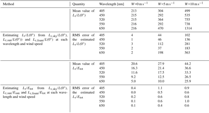
The results of this procedure have been presented in Fig. 8 and Table 7. The RMS values of the errors are≤0.0001 at all wind speeds≤10 m s−1, while the RMS errors relative to the mean values ofLr/Etot are ≤5%, which should be
ac-ceptable deviations. Table 7 shows the spectral results for the method where onlyL(0◦) is used as a reference, and the method whereL(0◦) is supplied by observations ofEtot. We
see that in our case with zenith-reflected radiance and signifi-cant contributions from sun glints at the studied wind speeds, satisfactory results can only be obtained by the latter method. Values of the ratio between the water-leaving radiance and the reflected radiance,Lw/Lr, have been tentatively
Table 7. Comparison of mean values and RMS errors ofLr/L(0◦) andLr/Etotin units of 10−4by different methods for estimating the
reflected radiance.
Method Quantity Wavelength [nm] W=0 m s−1 W=5 m s−1 W=10 m s−1
Mean value of Lr/L(0◦)
405 450 520 550 650 213 215 215 216 216 304 292 364 292 470 499 535 755 738 1314
Estimating Lr/L(0◦) from Lr,sky/L(0◦),
Lr,sun/L(0◦)) and Lr,foam/L(0◦) at each
wavelength and wind speed
RMS error of the estimated Lr/L(0◦)
405 450 520 550 650 4 1 3 2 2 44 46 112 37 198 102 136 281 183 563
Mean value of Lr/Etot
405 450 520 550 650 20.6 16.3 11.6 9.2 5.0 27.9 21.4 17.5 12.5 10.0 44.2 36.6 33.3 26.5 25.9
Estimating Lr/Etot from Lr,sky/L(0◦),
Lr,sun/EsunandLr,foam/Etotat each
wave-length and wind speed
RMS error of the estimated Lr/Etot
405 450 520 550 650 0.4 0.0 0.2 0.1 0.1 1.1 0.5 0.6 0.6 0.4 0.9 0.6 0.8 1.0 0.6
values ofLr/Etot. For the calculation of Lr/Etot an
atmo-spheric data set was chosen whereθs was as close to the cor-responding angle forLw/Etotas possible, and the calculation
was made with the same wind speed as forLw/Etot. The wind
speed at the selected stations varied from 1.5 to 7.5 m s−1and
the solar zenith angle from 37◦to 52◦. The results, presented in Table 6, show that within the spectral range 405–650 nm neither of the contributionsLw orLr to the zenith-directed
radiance can be disregarded relative to the other one in the Oslofjord-Skagerrak area.
This paper has discussed the case where the viewing direc-tion has been directed towards the nadir. If such recordings are made from a ship, the sensor must be mounted on a bar at a long distance from the rail, on the same side as the sun, in order to avoid the shadowing and reflecting effects of the ship. If the ship is at rest, a position in the direction back-wards from the stern minimizes the ship’s influence. If the ship is moving, the wake of the ship must be avoided, be-cause the reflecting properties of the wake are quite different from those of the sea around it. In addition to the nadir ra-diance from the sea, the zenith rara-diance from the sky as well as the downward irradiance must be recorded, and especially the irradiance sensor should be mounted as high as possi-ble, to avoid the influence of the ship building and masts. If the sensor is mounted up in a mast, its position should be as long away from the mast as practically possible, to avoid the shadow of the mast.
However, ship-mounted sensors usually have non-nadir viewing angles in order to avoid both the influence of the ship within the field-of-view and the sun glitter, but unfor-tunately the sensors on moving ferries are apt to experience very varying azimuth angles with regard to the sun. Accord-ingly it will be very useful to have simple methods for esti-mating the different types of reflected radiance: from the sky, sun and foam. In an on-going co-project with the Norwegian Institute for Water Research other angles than the nadir di-rection are studied. It is considered if observations in the ultraviolet and near infrared, where the water-leaving radi-ance in coastal water usually will be very small compared to the surface-reflected radiance, can be utilized for correction purposes. It has been demonstrated in this paper that if the ratiosLr,sky/L(0◦) andLr,sun/Esun are known at one
Acknowledgements. The author is due thanks to the topical editor and the referees for their constructive comments and suggestions. Edited by: P. Cipollini
References
Aas, E.: Calibration of a marine radiance and colour index meter, Rep. No. 87, Dept. Geophys., Univ. Oslo, 1993.
Aas, E. and Høkedal, J.: Reflection of spectral sky irradiance on the surface of the sea and related properties, Remote Sens. Environ., 70, 181–190, 1999.
Aas, E. and Højerslev, N. K.: Analysis of underwater radiance ob-servations: Apparent optical properties and analytic functions describing the angular radiance distribution, J. Geophys. Res., 104, 8015–8024, 1999.
Aas, E., Højerslev, N. K. and Høkedal, J.: Conversion of sub-surface reflectances to above-sub-surface MERIS reflectance, Int. J. Remote Sens., 30, 5767–5791, 2009.
Aas, E., Højerslev, N. K. and Lundgren, B.: Spectral irradiance, radiance and polarization data from the Nordic Cruise in the Mediterranean Sea during June-July 1971, Rep. No. 102, Dept. Geophys., Univ. Oslo, Norway, 1997.
Aas, E. and Korsbø, B.: Self-shading effect by radiance meters on upward radiance observed in coastal waters, Limn. Oceanogr., 42, 968–974, 1997.
Abramowitz, M. and Stegun, I. A.: Handbook of Mathematical Functions, Dover Publ., New York, 1970.
Adams, J. T., Aas, E., Højerslev, N. K., and Lundgren, B.: Compar-ison of radiance and polarization values observed in the Mediter-ranean Sea and simulated in a Monte Carlo model, Appl. Opt., 41, 2724–2733, 2002.
Austin, R. W.: The remote sensing of spectral radiance from below the ocean surface, edited by: Jerlov, N. G. and Steeman Nielsen, E.: Optical Aspects of Oceanography, Academic Press, London, 317–344, 1974.
Cox, C. and Munk, W.: Statistics of the sea surface derived from sun glitter, J. Mar. Res., 13, 198–227, 1954a.
Cox, C. and Munk, W.: The measurements of the roughness of the sea surface from photographs of the sun’s glitter, J. Opt. Soc. Am., 44, 838–850, 1954b.
Deschamps, P.-Y., Fougnie, B., Frouin, R., Lecomte, P., and Ver-waerde, C.: SIMBAD: a field radiometer for satellite ocean-color validation, Appl. Opt., 43, 4055–4069, 2004.
Fougnie, B., Frouin, R., Lecomte, P., and Deschamps, P.-Y.: Re-duction of skylight reflection effects in the above-water measure-ment of diffuse marine reflectance, Appl. Opt., 38, 3844–3856, 1999.
Frouin, R., Schwindling, M., and Deschamps, P.-Y.: Spectral re-flectance of sea foam in the visible and near-infrared: In situ measurements and remote sensing implications, J. Geophys. Res., 101, 14361–14371, 1996.
Gordon, H. R. and Ding, K.: Self-shading of water optical in-struments, Limn. Oceanogr., 37, 491–500, 1992.
Gordon, H. R. and Wang, M.: Surface-roughness considerations for atmospheric correction of ocean color sensors I: The Rayleigh-scattering component, Appl. Opt., 31, 4247–4260, 1992a.
Gordon, H. R. and Wang, M.: Surface-roughness considerations for atmospheric correction of ocean color sensors II: Error in the retrieved water-leaving radiance, Appl. Opt., 31, 4261–4267, 1992b.
Hooker, S. B., Lazin, G., Zibordi, G., and McLean, S.: An eval-uation of above- and in-water methods for determining water-leaving radiances, J. Atmos. Oceanic Techn., 19, 486–515, 2002. Højerslev, N. K. and Aas, E.: Spectral irradiance, radiance and po-larization in blue Western Mediterranean waters, in Ocean Op-tics XIII, Proc., 22-25 October 1996, Halifax, Canada, SPIE Vol. 2963, 138–147, 1997.
Høkedal, J. and Aas, E.: Observations of spectral sky radiance and solar irradiance, Rep. No. 103, Dept. Geophys., Univ. Oslo, Nor-way, 1998.
Kattawar, G. W. and Adams, C. N.: Errors in radiance calculations induced by using scalar rather than Stokes vector theory in a real-istic atmosphere-ocean system, in Ocean Optics X, Proc., 16-18 April 1990, Orlando, Florida, SPIE Vol. 1302, 2–12, 1990. Koepke, P.: Effective reflectance of oceanic whitecaps, Appl. Opt.,
23, 1816–1824, 1984.
Kokhanovsky, A. A.: Spectral reflectance of whitecaps, J. Geophys. Res., 109, C05021, doi:10.1029/2003JC002177, 2004.
Lauscher, F.: Sonnen- und Himmelstrahlung im Meer und in Gew¨assern, edited by Linke, F. and M¨oller, F.: Handbuch der Geophysik, 8, Physik der Atmosph¨are, Gebr¨uder Borntraeger, Berlin, Germany, 723–768, 1955.
Lundgren, B.: On the polarization of the daylight in the sea, Rep. No. 17, Dept. Phys. Oceanogr., Univ. Copenhagen, 1971. Mobley, C. D.: Estimation of the remote-sensing reflectance from
above-surface measurements, Appl. Opt., 38, 7442–7455, 1999. Monohan, E. C.: Oceanic whitecaps, J. Phys. Oceanogr., 1, 139–
144, 1971.
Monohan, E. C. and O’Muircheartaigh, I. G.: Optimal power-law description of oceanic whitecap coverage dependence on wind speed, J. Phys. Oceanogr., 10, 2094–2099, 1980.
Monohan, E. C. and O’Muircheartaigh, I. G.: Improved state-ment of the relationship between surface wind speed and oceanic whitecap coverage as required for the interpretation of satellite data, edited by: Gower, J. F. R.: Oceanography from space, Plenum, New York, 751–755, 1981.
Monohan, E. C. and O’Muircheartaigh, I. G.: Whitecaps and the passive remote sensing of the ocean surface, Int. J. Remote Sens., 7, 627–642, 1986.
Moore, K. D., Voss, K. J. and Gordon, H. R.: Spectral reflectance of whitecaps: Instrumentation, calibration, and performance in coastal waters, J. Atmos. Oceanic Technol., 15, 496–509, 1998. Moore, K. D., Voss, K. J., and Gordon, H. R.: Spectral reflectance
of whitecaps: Their contribution to water-leaving radiance, J. Geophys. Res., 105, 6493–6499, 2000.
Morel, A.: In-water and remote measurements of ocean color, Bound.-Layer Meteor., 18, 177–201, 1980.
skew-ness of surface slopes, Ann. Rev. Mar. Sci., 1, 377–415, 2009. Nicolas, J.-M., Deschamps, P. Y., and Frouin, R.: Spectral
re-flectance of oceanic whitecaps in the visible and near infrared: Aircraft measurements over open ocean, Geophys. Res. Lett., 28, 4445–4448, 2001.
Preisendorfer, R. W. and Mobley, C. D.: Albedos and glitter patterns of a wind- roughened sea surface, J. Phys. Oceanogr., 16, 1293– 1316, 1986.
Ruddick, K. G., De Cauwer, V., and Park, Y.-J.: Seaborne measure-ments of near infrared water-leaving reflectance: The similarity spectrum for turbid waters, Limnol. Oceanogr., 51, 1167–1179, 2006.
Tyler, J. E.: Radiance distribution as a function of depth in an un-derwater environment, Bull. Scripps Inst. Oceanogr., 7, 363–412, Univ. Cal., La Jolla, Cal., 1960.
Walker, R. E.: Marine Light Field Statistics, Wiley, New York, 1994.
Whitlock, C. H., Bartlett, D. S., and Gurganus, E. A.: Sea foam re-flectance and influence on optimal wavelength for remote sensing of ocean aerosols, Geophys. Res. Lett., 9, 719–722, 1982.
Wu, J.: Oceanic whitecaps and sea state, J. Phys. Oceanogr., 9, 1064–1068, 1979.
Zibordi, G. and Ferrari, G. M.: Instrument self-shading in under-water optical measurements: experimental data, Appl. Opt., 34, 2750–2754, 1995.
Zibordi, G., Hooker, S. B., Berthon, J. F., and D’Alimonte, D.: Au-tonomous above- water radiance measurements from an offshore platform: a field assessment experiment, J. Atmos. Ocean. Tech., 19, 808–819, 2002.
Zibordi, G., M´elin, F., Hooker, S. B., D’Alimonte, D., and Hol-ben, B.: An autonomous above-water system for the validation of ocean color radiance data, IEEE Trans. Geosc. Remote Sens., 42, 401–415, 2004.