On the usefulness of
E
region electron temperatures and lower
F
region ion temperatures for the extraction of thermospheric
parameters: a case study
J.-P. St.-Maurice1, C. Cussenot2, W. Kofman2
1 Department of Physics and Astronomy, The University of Western Ontario, London, Ontario N6A 3K7, Canada 2 LIS, URA 342, BP-46, 38402 Saint Martin d'heÁres Cedex, France
Received: 21 October 1998 / Revised: 20 January 1999 / Accepted: 3 February 1999
Abstract Using EISCAT data, we have studied the
behavior of theEregion electron temperature and of the
lowerF region ion temperature during a period that was
particularly active geomagnetically. We have found that
the E region electron temperatures responded quite
predictably to the eective electric ®eld. For this reason,
the E region electron temperature correlated well with
the lower F region ion temperature. However, there
were several instances during the period under study
when the magnitude of the E region electron
tempera-ture response was much larger than expected from the ion temperature observations at higher altitudes. We discovered that these instances were related to very strong neutral winds in the 110±175 km altitude region.
In one instance that was scrutinized in detail using E
region ion drift measurement in conjunction with the temperature observations, we uncovered that, as sus-pected, the wind was moving in a direction closely matching that of the ions, strongly suggesting that ion drag was at work. In this particular instance the wind reached a magnitude of the order of 350 m/s at 115 km and of at least 750 m/s at 160 km altitude. Curiously
enough, there was no indication of strong upper F
region neutral winds at the time; this might have been because the event was uncovered around noon, at a time
when, in the F region, the EB drift was strongly
westward but the pressure gradients strongly northward
in theF region. Our study indicates that both the lower
F region ion temperatures and the E region electron
temperatures can be used to extract useful geophysical parameters such as the neutral density (through a determination of ion-neutral collision frequencies) and Joule heating rates (through the direct connection that we have con®rmed exists between temperatures and the eective electric ®eld).
Key words. Ionosphere (auroral ionosphere; ionosphere atmosphere interactions; plasma temperature and density)
1 Introduction
It has been repeatedly pointed out that the ion temperature below 400 km altitude depends quadratic-ally on the magnitude of the relative drift between ions and neutrals (e.g., Rees and Walker, 1968; St.-Maurice and Hanson, 1982, 1984). However, it may not have been stressed strongly enough that this is equivalent to the ion temperature having a quadratic dependence on
the magnitude of the eective electric ®eld
E0EVnB. Thayer (1998a, b) recently emphasized
that the actual Joule heating rate that determines a large fraction of the rate at which energy is transferred from the magnetosphere to the thermosphere actually de-pends on the magnitude of the eective electric ®eld
through R
rP zj jE02dz where z is the altitude and rP is
the height-dependent Petersen conductivity. The ion temperatures obtained with incoherent scatter radars should therefore in principle, provide an accurate description of the Joule heating rates without even the need for drift measurements. However, as we discuss in more detail below, things are not so simple: on the one hand, the temperature enhancements have to be large enough to avoid large uncertainties associated with neutral temperature models and error bars on the measurements. On the other hand, when the tempera-ture enhancements are large, the ion velocity distribu-tion becomes anisotropic and non-Maxwellian which complicates the analysis sometimes considerably. For these reasons, the ion temperatures may have been overlooked as a useful tool for monitoring the state of the thermosphere. But with considerable progress made on data processing and analysis together with a much
clearer characterization of non-Maxwellian features the time has come to give the ion temperature another shot. A similar situation has evolved with electron
tem-peratures in the E region. As we discuss in more detail
below, it is now clear that for electric ®elds of the order of 40 mV/m or greater the electron temperature rapidly climbs up well above the neutral and ion temperatures. Much emphasis has been given to producing an expres-sion for the heating rates using nonlinear plasma physics, at the expense of exploring the possibilities that the enhancements can provide as a tool to study the thermosphere. Later in this paper we show that one can argue on theoretical grounds that the electrons, like the ions, respond to the eective electric ®eld rather than to the electric ®eld itself. This would imply that the electrons could be used to monitor the Joule heating rates in an altitude range that is particularly important for magnetospheric energy deposition rates. Again, we wish to argue here that knowledge and technology have now both progressed to the point that this is entirely feasible.
One of the features that may have hindered progress in terms of utilizing electron temperatures is that, contrary to what has been obtained with small data subsets over several hours of data acquisition, the electron temperature data often exhibit a large amount of scatter when plotted against the electric ®eld strength. This has been blamed in the past mostly on poor electric
®eld estimates (St.-Maurice et al., 1990; Haldoupis
et al., 1993; Williams et al., 1992). Since many radar experiments do not monitor the electric ®elds on as short a time-scale as the temperatures, this may have led to a lack of study of many a data set. It may be, however,
that much of the scatter inTeversus electric ®eld plots is
actually of a geophysical rather than statistical nature. One is reminded of a similar problem that was faced by St.-Maurice and Hanson (1984) when looking at large data sets of ion temperatures onboard the AE-C satellite: as the electric ®eld was increasing the ion temperatures would exhibit increasingly large standard deviations about a mean that was close to the values expected for zero neutral winds. The source of the scatter was identi®ed with neutral wind values of fairly normal magnitudes aecting the temperature response through simple changes in the angle between winds and ion drifts. Given that there is a strong theoretical case for the electron temperature to also respond to the eective electric ®eld and not the ®eld itself one is left
wondering about that possibility for the E region
electron temperatures as well.
Our most important goal in this paper is therefore to
document the eective electric ®eld dependence of theE
region electron temperature based on EISCAT radar observations of the phenomenon. To this end we will present results from 24 h of data acquired during an extremely geomagnetically disturbed period. In the process of making our case, we will also show that the behavior of the ion temperature is now understood well enough to extract reliable values for the eective electric
®eld throughout the upper E region and the lower F
region. We will in fact show how the ion-neutral collision frequency can be extracted from the ion
temperature and drift behavior in theEregion, implying
that once calibrated, the electron temperatures below 120 km could be used to extract this information more easily and quite reliably during heating events. Finally, we will also present, using the principles we uncovered, one example for which we extracted neutral winds of
exceptional magnitudes in the E region and lower F
region. The data in that case was strongly indicative of a strong ion drag eect, which did not seem, however, to
extend to upperF region heights.
Before presenting our particular data set and our analysis of it we will review brie¯y in sect. 2 the basis for using ion and electron temperatures as proxies for the eective electric ®eld strength. This is followed in sect. 3 by a description of the particular experiment that we used and an overview of the data that were acquired. In sect. 4 we focus on a rather striking feature of our particular data set in which an `upper electron temper-ature branch' (UTEB) clearly emerges from the rest of the data. From a detailed study of the available data
during UTEB events we will show that very strong E
region neutral winds were aecting both the ion and the electron temperature data, but more so the ions above 130 km altitude. Further evidence that this was indeed the case is presented in sect. 5, where we have extended our method to include the observation of ion drift vectors during a particular time interval for which the electric ®eld did not change.
2 The connection between ion and electron temperatures and the eective electric ®eld strength
2.1 Ions
The dominant terms in the ion energy balance below 400 km altitude are the frictional heating term and the heat exchange term with the neutrals. The lower the altitude the truer this becomes. The equation that results from this balance is, to a good approximation, given by (e.g., St.-Maurice and Hanson, 1982)
TiTn
hmni
3Kb
ViÿVn
2 1
where Ti and Tn are the ion and neutral temperatures
respectively, Kb is the Boltzmann constant, Vi and Vn
are the ion and neutral drifts respectively andhmniis a
collision-frequency-weighted average neutral mass.
We can also writeTi in terms of the eective electric
®eldE0EVnB. As we show in the Appendix, Eq.
(1) can then be replaced by
TiTn
hmni
3Kb
E0=B 2
1a2
i
2
where aimi=Xi is the ion collision to cyclotron
frequency ratio. The merit of Eq. (2) is to express
explicitly thatTidepends strictly on the eective electric
Equation (2) implies that, to obtain the magnitude of the eective electric ®eld and its altitude variation, one
``simply'' has to study the variation of Ti with altitude.
Things are not quite that straightforward in practice, however; even with an ideal situation where radar spectra would have excellent signal-to-noise ratio, there are several diculties to wrestle with. For one thing
both Tn and hmni are altitude-dependent, particularly
between 175 and 225 km, where the dominant neutral
switches from N2 to O while Tn undergoes a transition
from radiation-dominated to heat-¯ow-dominated. To make things worse, during active conditions, Joule heating eects lead to increases in the neutral
temper-atures and to increases in the average N2 to O
composition ratio, at all F region heights. This all
conspires to make an accurate description of the altitude
dependence of Ti much more dicult in the altitude
transition region where the dominant neutral switches
from N2 to O.
Another complication, which becomes important when the electric ®eld is large, is that the ionospheric ion temperature becomes anisotropic and the ion velocity distribution becomes non-Maxwellian, with a larger temperature value perpendicular versus along the
magnetic ®eld direction (e.g., Gaimard et al., 1998).
Therefore, if, as will be the case here, one is to use measurements made along the magnetic ®eld to deter-mine the ion temperature, one has to remember that the line-of-sight temperature will actually be smaller than the average ion temperature given by Eqs. (1) or (2). Speci®cally, the parallel temperature can be adequately described by the equation
Tik Tn
hmni
3Kb
E0=B 2
1a2
i
1:5bk 3
Unfortunately, the value ofbkchanges signi®cantly both
with ion and neutral composition. For the N2
dominat-ed atmosphere below 175 km we will be following
McCrea et al. (1993) and use bk 0:52 (as opposed to
2/3 for a spherically symmetric distribution). From the same work, but for the oxygen-dominated atmosphere
above 250 km, bk should be between 0.18 and 0.25
when dealing with Oions. Note that the bk diculties
notwithstanding, the parallel ion temperature still theoretically increases quadratically to ®rst order with the eective electric ®eld strength.
There remains the actual non-Maxwellian shape of the ion velocity distribution to deal with. This aects the radar spectra and is more dicult to model because the spectral shape is a function of both the electron-to-ion temperature ratio and of the ion mass. Both change with altitude but unfortunately in a somewhat unpredictable manner, particularly at high latitudes. Nevertheless, using theoretical and Monte-Carlo calculations, it has been shown that the non-Maxwellian spectra can be inverted particularly if the signal to noise is of good quality and if the angle between the line of sight and the
magnetic ®eld is not too steep (e.g., Winkleret al., 1992;
Hubert and Lathuillere, 1989). It also helps to be in
situation where N2 is the dominant neutral constituent
because in that case the departures from a Maxwellian shape are not as large nor as dicult to model as when the background neutral gas is O.
The above implies that it is easier to use the ion temperature to retrieve the magnitude of the eective electric ®eld at altitudes ranging between 130 km and 175 km. The main reasons for this are (1) above 130 km
ai is small so that the magnitude of the temperature
response is at its largest and (2) the dominant neutral
atmospheric constituent in that case is N2 for sure. The
advantages of being in a region where N2is the dominant
neutral are many: for one thing, a larger mean neutral
mass,hmni, increases the magnitude of the ion
temper-ature response to the electric ®eld (see Eq. 2). For another, it removes the uncertainty in the average neutral mass, which can be highly variable above 180 km in the auroral region and can therefore introduce modulations
in the response ofTito the eective electric ®eld strength.
And ®nally, the ion composition is also dominated by
NO ions when the neutrals are mostly N2 (i.e., below
170 km for sure), which removes some further ambiva-lence with respect to the interpretation of non-Maxwell-ian ion line spectra. This being said, we will not go as far as to attempt to correct for non-Maxwellian distortions although we will consider anisotropic ion temperature eects. Our neglect of other non-Maxwellian distortions should not create a systematic eect, although it will admittedly be introducing some additional scatter in the data (e.g., Lathuillere and Hubert, 1989).
2.2 Electrons
Schlegel and St.-Maurice (1981) and Wickwar et al.
(1981) discovered that, if the electric ®eld strength exceeds about 40 mV/m at high latitudes, the electron temperature around 105±115 km is correlated with the electric ®eld strength (while being generally anti-corre-lated with electron precipitation at those heights). These basic results were con®rmed by many subsequent studies
(see review by St.-Mauriceet al. (1990) for papers prior
to 1990; also see Joneset al., 1991; Williamset al., 1992;
Haldoupiset al., 1993) and are now accepted as a fact of
components along the magnetic ®eld that are large enough to heat the electrons to produce the observed temperatures (e.g., St.-Maurice and Laher, 1985).
Whatever the detailed mechanism, one could look at the problem this way: in a steady-state situation, the power going through large amplitude plasma waves has to go back to particles. Since the power going to the waves is actually dominated by Joule dissipation even in the linear growth stages (St.-Maurice, 1987), one has to conclude that the electron heating rate should be related to the eective electric ®eld at least quadratically once unstable waves are triggered (we show in the Appendix that the heating rate depends on the eective electric ®eld even though the instability extracts its power from the currents). The heating rate may very well go up even faster because (1) the electron-neutral collision frequen-cy, on which the heating rate depends linearly, also changes dramatically with the electron temperature itself and (2) an increasingly large range of unstable modes is excited as the ambient electric ®eld increases (Kissack et al., 1997). In other words, once it is recognized that the plasma waves can reach a large enough amplitude to heat the electrons, the heating rate can only increase rapidly (at least quadratically) with eective electric ®eld strength. One more observation deserves a mention: since the eective electric ®eld is not normally expected to change much with altitude below 115 km and since the heating and cooling rates are otherwise both proportional to the neutral density, the only reason why the electron temperature goes down at all as we go from 115 km down to 100 km is that the power going through the waves must also be going down. This is consistent with the fact that the linear growth rates are known to become smaller as we go down in altitude.
At any rate, as far as a precise quantitative descrip-tion of the electron temperature is concerned our approach in the present paper will be similar to the
one taken by St.-Mauriceet al. (1990), namely, we will
simply rely on the data itself to infer the relation between the electron temperature and the eective electric ®eld strength.
3 Description and overview of the observations
The data were obtained during a 25-h UHF (980 MHz) EISCAT run that started at 10 UT on 9 April 1990. The Tromso radar, where the transmitter is located, recorded spectra along the magnetic ®eld line for the duration of the experiment. A multipulse oering a 3-km resolution with 2.7-km range-stepping was used between 90 km and 250 km altitudes. A long pulse with a 22 km range step and 54 km altitude resolution was also used to cover the altitude range 150±600 km. For this paper we used a 1 min integration time with the analysis of the Tromso data.
The remote stations at Kiruna and Sodankyla were used in a scanning mode that intersected the Tromso geomagnetic ®eld lines at seven particular altitudes: 90 km, 95.5 km, 100.5 km, 108 km, 116.2 km, 124 km and 278 km. The 278 km altitude gate provided a
measurement of the plasma EB drift vector while
the lower altitudes were used to determine the ion drift in regions where the ions were unmagnetized or, at most, only partially magnetized. The altitude scan mode was
such that the EB drift could be sampled at 5-min
intervals.
Below 108 km altitude, at the UHF frequency used for the data analysis presented here, the shape of the ion line spectrum is aected by ion-neutral collisions, which tend to drive a Lorentzian shape, as well as by the ratio
Te=Ti, which tends to drive a double-hump spectrum if
Te>Ti. It is not possible to solve for ion-neutral
collisions and for the ratio Te=Ti simultaneously.
In-stead, one either solves for the collision frequency
assuming TeTi, or one ®xes the collision frequency
and solves for the individual temperatures. In this latter case we use an empirical collision frequency model derived under similar conditions, but in the absence of
strong electric ®eld (Kofmanet al., 1986). We note that
the essential quantitative results that we will present here will depend on the ion and electron temperatures obtained above 108 km anyway, so that any uncertainty introduced by the use of our empirical collision model will only have minimal impact on what we shall present. A second factor could aect the data interpretation, namely, the ion composition. Unless a whole pro®le is being ®tted, which is not the case here, we have to rely on a composition model to determine the ion temperature. This is because the spectrum basically yields the value of
the thermal speed, which is proportional to Ti=mi
p
where mi represents the mean ion mass. In the altitude
range 150±250 km the ion goes from all molecular
NO to basically all atomic O. In order to avoid
complications with composition uncertainties (which are compounded by chemical eects during ion heating events), we have limited our study for the most part to altitudes either greater than 250 km or less than 170 km, deriving the ion temperatures using a standard EISCAT composition model. This means that, for instance, at
168 km, we have assumed that the NO to ne density
ratio was 0.83. During heating events associated with large electric ®elds, the molecular ion concentration should increase, and it is likely that the ratio will increase above 0.83. However, judging from statistical studies (Lathuillere and Pibaret, 1992) as well as a case study (Lathuillere, 1987) it seems very unlikely that at 168 km the ratio will exceed 0.90. For multipulse data, the
related possible underestimation in Ti at 168 km will
therefore be less than 15% for sure, and very likely be less than half that value in fact. However, for long pulse data centered on 168 km, the possible uncertainties will in principle be larger because of pulse smearing eects. This being said, a variation in excess of 15% still seems to be unlikely even in that case. Finally, for multipulse data lower down, also note that for altitudes 150 km and less, the composition model we used is already more than
95% NO below 150 km altitude. This implies that the
analyzed Ti is not aected by ion heating-induced
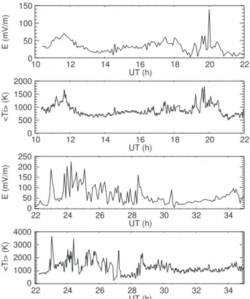
of the EB drift sampled by the remote stations changed with time during the period of observation. For comparison, we also display on the same time-scale the behavior of the parallel ion temperature. The ion temperature was sampled every minute, which makes for the higher density of points. Also, because of the degree of noise associated with the multipulse we took an altitude average of the ion temperature between the 140 and 160 km altitude gates as well as a 3-point running-average in time. In spite of the smoothing brought by this procedure, there is little doubt that
many of the50K oscillations in the resulting plot are
due to noise. Notice also that bad data points were excluded and that this led at times to larger jumps between points. Not surprisingly, there was a tendency for bad data points to be observed when the electric ®eld was highly structured in time and the ion density was simultaneously small, resulting in autocorrelation func-tions that could not be satisfactorily ®tted, probably because of poor signal-to-noise ratios.
Figure 1 illustrates that the electric ®eld exceeded 100 mV/m on several occasions, particularly around
midnight (around the time that theAp index reached its
maximum value of 207 for the event). The measured
EBdrift actually exceeded 3 km/s on a few occasions
and even went beyond 4 km/s in one case. This result is remarkable in that very strong electric ®elds are usually dicult to catch because of their high localization and short lifetime. As a result, it is quite reasonable to expect
that particularly in the time interval 24:00±25:00 UT the ®eld may well have reached or exceeded the 200 mV/m value on more than one occasion.
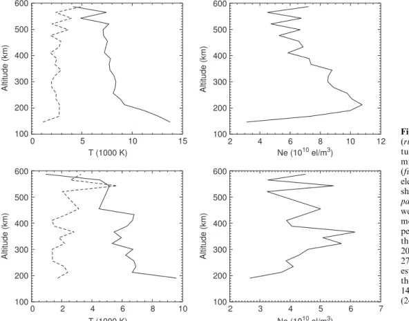
To show that the inference of very strong electric ®elds was indeed strongly supported by other features in the data, we present in Fig. 2 two pro®les of the ion temperature for the long pulse data taken during the time interval over which the electric ®eld was reaching very large values. As Fig. 2 shows, consistent with our expectations of exceptional electric ®elds, the long pulse data reported parallel ion temperatures in excess of 12,000 K below 200 km altitude in the examples shown. (Notice that the signal-to-noise ratio was too small for the multipulse to produce useful estimates during that time). At the times of the posted observations, the electric ®eld estimated from the 278 km altitude ion drift measurement reached 225 mV/m (top panel) and 141 mV/m (bottom panel). Notice how the parallel ion temperature above 200 km was substantially less than lower down. This is mainly due to the mean mass factor
in Eq. (1), which is dominated by N2below 175 km and
by O above 200 km. A similar kind of ion temperature pro®le behavior under very strong electric ®eld condi-tions was in fact reported earlier by Kofman and Lathuillere (1987).
Figure 1 illustrates that the selected experimental mode suered some drawbacks when the electric ®eld became very strong for the case under study. We refer here to the large point by point oscillations in the electric ®eld data on the 5-min time-scale that could be observed particularly around 24:00 UT. These oscillations indi-cate that the strong electric ®elds were highly variable over the 5-min time-scale, and that it was risky at best to try to even interpolate the data to get the electric ®eld variations on shorter time scales during that time period. This means that we had to fall back on the temperature measurements to monitor the magnitude of the electric ®eld on shorter time scales. Thus, the ion temperatures obtained with the long pulse along the geomagnetic ®eld line was not only giving a better temporal resolution, but was also better able to track the electric ®eld strength than the drift measurements, at least during periods of reduced ion densities. This being said, one should note the general correlation between the parallel ion temperatures and the drift-deduced electric ®eld strength in Fig. 1, as expected from Eqs. (1) or (3). Thus, there was general agreement between the two measure-ments, but some of the details diered. In our in-depth analysis, such details could be important, as we shall illustrate in sect. 4.
4 The detailed response ofTi andTeto electric ®eld variations
4.1 Results from scatter plots
For the reasons presented in sect. 2, both the ion temperature around 150±160 km altitude and the
elec-tron temperature in theEregion could be expected to be
good indicators of the electric ®eld strength if, as is often 0
50 100 150
22
22
34
34 20
20
32
32 18
18
30
30 16
16
28
28 14
14
26
26 12
12
24
24 10
10
22
22
UT (h)
UT (h)
UT (h)
UT (h)
E (mV/m)
E (mV/m)
0 1000 2000 3000 4000
<Ti> (K)
<Ti> (K)
0 50 100 150 200 250 0 500 1000 1500 2000
assumed, the role played by the neutral wind was not
too important at E region heights. For this reason we
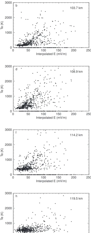
®rst produced scatter plots of the multipulse-derived Te
versus the electric ®eld strength at various E region
altitudes (Fig. 3a). To estimate the electric ®eld, we used
a simple linear interpolation technique when theTedata
was not obtained simultaneously with an electric ®eld measurement. One can see a general trend from Fig. 3a
for Te to increase with electric ®eld strength. There is a
central `cloud' of data points, but the scatter around that cloud can be substantial. Given the discussion in the preceeding section on the unreliability of interpo-lated electric ®elds around the times of strongest electric ®elds we can easily suspect that the electric ®eld determination itself was error prone when large, which would perhaps explain some of the scatter.
On the other hand, we already argued that the electron temperature should depend on the eective electric ®eld and not on the electric ®eld itself. For this
reason, we compared the electronEregion temperatures
to the ion temperature around 160 km. The latter was
chosen because at that height the Ti response to the
eective electric ®eld is the largest [the neutral mass in
Eq. (2) being the largest, that is, made mostly of N2
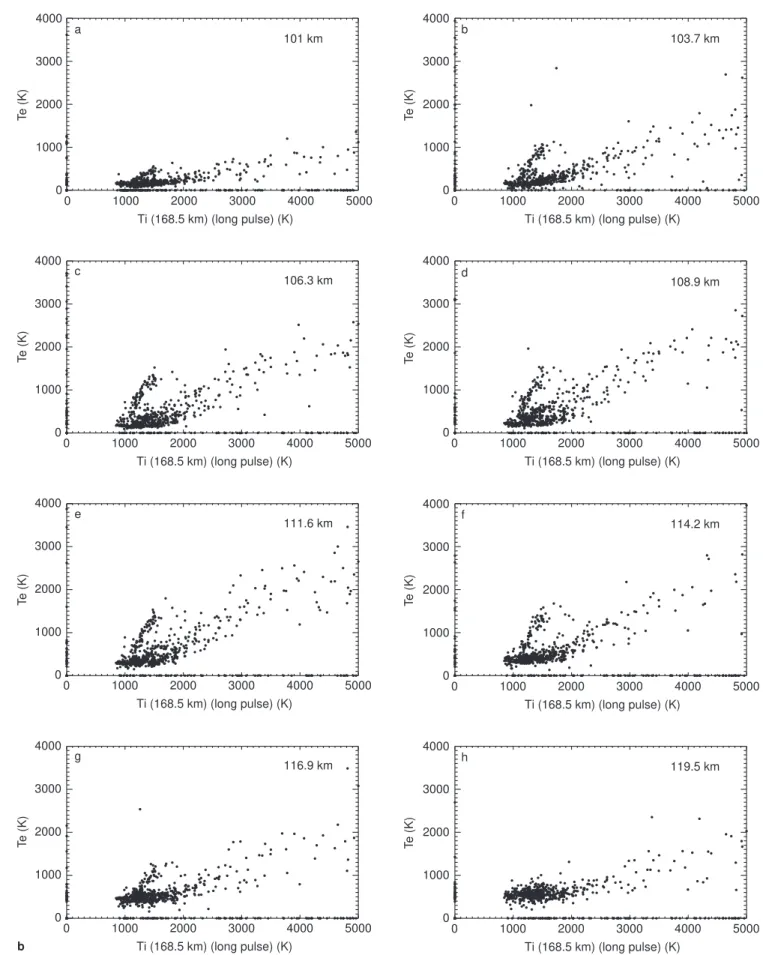
while ai!0]. We ®rst produced scatter plots of the
multipulse E region electron temperatures versus Ti
obtained using the multipulse ion data, averaging the latter over 10 km centered at 160 km. Unfortunately, the result was actually rather noisy. To see if we could
clean up the scatter in theTevsTiplots, we then kept the
E-region electron multipulse data (rather good signal to
noise ratio compared to multipulse Ti data higher up),
but tried the long pulse Ti data at the 168-km gate
instead of the multipulse data. We obtained the results
displayed in Fig. 3b. While the multipulse Ti data gave
similar trends, the scatter found with the long pulse data was indeed much smaller, most likely owing to its much better signal to noise ratio. As a comparison between Figs. 3a and 3b shows, the data points were also
scattered a lot less by using the long pulse Ti data at
168 km than when we used the interpolated electric ®eld. Partly because of the removal of any interpolation
technique and probably also in part because theTi data
depends, like theTe data, on the eective electric ®eld,
and not on the electric ®eld itself, the long pulse low
altitudeTidata appeared to be the best at predicting the
E region electron temperature by showing the least
scattering and by getting rid of virtually all lowTe-high
electric ®eld cases. However, Fig. 3b clearly shows that this was done at the expense of introducing an `anom-alous branch' in the electron temperature behavior. A discussion of the plausible physics behind such a branch is the topic of the next subsection.
Before moving to an in-depth discussion of Fig. 3b, the reader should also be aware that Fig. 3 was produced by using the second half of the night only, that is, the time interval 22:00±35:00 UT. The ®rst half of the night actually gave similar trends, in fact with an even greater percentage of `anomalous' data points, but with a greater amount of scattering. We believe from the analysis that follows that this scattering was actually of geophysical origin. We therefore decided to stick with 100
100 100
100 200
200 200
200 300
300 300
300 400
400 400
400 500
500 500
500 600
600 600
600
15 10
5 0
Altitude (km)
Altitude (km) Altitude (km)
Altitude (km)
T (1000 K)
T (1000 K)
10 8 6 4 2 0
12 10 8 6 4 2
Ne (1010el/m )3
Ne (1010el/m )3
7 6 5 4 3 2
Fig. 2. Example of density (right-hand-side) and tempera-ture pro®les (left-hand-side) with much larger ion temperatures (full lines) than average. The electron temperatures are also shown on theleft-hand-side panels(dashed lines). The times were taken in the middle of the most disturbed interval for the period under study, taken when theAp index reached a value of
a
c
e
g h
f d b
0
0
0
0 0
0 0 0 1000
1000
1000
1000 1000
1000 1000 1000 2000
2000
2000
2000 2000
2000 2000 2000 3000
3000
3000
3000 3000
3000 3000 3000
250
250
250
250 250
250 250 250 200
200
200
200 200
200 200 200 150
150
150
150 150
150 150 150 100
100
100
100 100
100 100 100 50
50
50
50 50
50 50 50 0
0
0
0 0
0 0 0 Interpolated E (mV/m)
Interpolated E (mV/m)
Interpolated E (mV/m)
Interpolated E (mV/m) Interpolated E (mV/m)
Interpolated E (mV/m) Interpolated E (mV/m) Interpolated E (mV/m)
T
e (K)
T
e (K)
T
e (K)
T
e (K)
T
e (K)
T
e (K)
T
e (K)
T
e (K)
101 km
106.3 km
111.6 km
116.9 km 119.5 km
114.2 km 108.9 km 103.7 km
a
a
c
e
g h
f d b
T
e (K)
T
e (K)
T
e (K)
T
e (K)
T
e (K)
T
e (K)
T
e (K)
T
e (K)
101 km
106.3 km
111.6 km
116.9 km 119.5 km
114.2 km 108.9 km 103.7 km
0 0
0
0
0 0
0 0
1000 1000
1000
1000
1000 1000
1000 1000
2000 2000
2000
2000
2000 2000
2000 2000
3000 3000
3000
3000
3000 3000
3000 3000
4000 4000
4000
4000
4000 4000
4000 4000
5000 5000
5000
5000
5000 5000
5000 5000
4000 4000
4000
4000
4000 4000
4000 4000
3000 3000
3000
3000
3000 3000
3000 3000
2000 2000
2000
2000
2000 2000
2000 2000
1000 1000
1000
1000
1000 1000
1000 1000
0 0
0
0
0 0
0 0
Ti (168.5 km) (long pulse) (K) Ti (168.5 km) (long pulse) (K)
Ti (168.5 km) (long pulse) (K)
Ti (168.5 km) (long pulse) (K)
Ti (168.5 km) (long pulse) (K) Ti (168.5 km) (long pulse) (K)
Ti (168.5 km) (long pulse) (K) Ti (168.5 km) (long pulse) (K)
b
the second half of the night in what follows because of the more unambiguous message that it provided, thanks to its smaller amount of scatter.
4.2 De®ning and isolating UTEB events
As was just mentioned, a striking feature of the scatter
plots shown in Fig. 3b is the appearance of an `upperTe
branch' (UTEB) which is clearly noticeable between 101 km and 117 km altitude. The UTEBs form an `anomaly' not just because they don't behave like the majority of the data, but also because they show electron temperatures that are well above the values that have previously been reported in the literature (as
deduced here by takingTikand Eq. (3) to ®nd the electric
®eld strength).
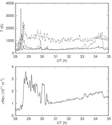
The UTEB data did not come from isolated single point measurements. Rather, as might be expected, the data was regrouped around certain UT periods. Fig-ure 4 illustrates this clearly. In Fig. 4, we produced a
time sequence of the averageTebetween 106 and 116 km
(dashed line), the average Ti between 106 and 116 km
altitudes (full line) and the averageTi between 140 and
160 km (dash-dot line). The most obvious UTEB event for the displayed time interval started around 33:00 UT and peaked around 34:30 UT. The event was quite
clearly taking place while the averageTi around 150 km
only suered a modest increase. In fact, for Te to have
reached more than 1000 K as shown at the peak of the
event,Ti at 150 km should have been well in excess of
2000 K, as illustrated by the `normal' features observed before 29:00 UT (also see the scatter plot in Fig. 3b to con®rm this point).
Also shown in Fig. 4 is the average electron density between 106 and 116 km, showing that there was a nice correlation between the 34:00 UT UTEB and the electron density in the same region. This kind of connection should not be viewed as a cause of UTEB, however, but rather as its consequence. The phenome-non has in fact previously been discussed and is due to the reduced recombination rates that one is to expect in the presence of electron production and of electron
heating (St.-Mauriceet al., 1990; Schlegel, 1982). This is
a particularly clearcut example of the phenomenon, since the source of electrons was known rather precisely for the time interval under consideration: detailed model calculations show that photoionization was by far the dominant source of electrons at the time (P.L. Blelly, private communication). This is also easy to see from
the steady climb in the background E region density
starting at about 31:00 UT.
4.3 Neutral winds as the likely origin of UTEBs
Given that the theory of electron heating by plasma waves is not yet fully understood, one could think that the UTEBs might be linked to periods during which the plasma wave generation could have been dierent, and with it the nonlinear properties of the waves and the associated electron heating (for example, gradients could have somehow become important during the UTEBs in such a way as to change the wave amplitude). However, one could also explain the UTEB generation with the production of strong enough neutral winds in the plasma, thus making the eective electric ®eld altitude-dependent. Based on the detailed observations surrounding UTEB events, we show in the present section that the latter explanation is very likely to be the correct one. This in turn suggests that the electron temperature may well be a robust indicator of the eective electric ®eld strength.
4.3.1 Mean electric ®eld values
The ®rst indication that neutral winds at 150 km are likely the reason for the UTEBs comes from the few electric ®eld measurements that were obtained during UTEBs. To determine these ®elds we proceeded as
follows: we ®rst produced eight 60 K wide Ti bins
between 1005 K and 1545 K from the long pulse data (our particular choice of bins was such as to have roughly the same number of samples in each bin, which
was typically 8). Next, for eachTi bin we looked at the
average interpolated electric ®eld strength that was observed during a UTEB (we picked the 106.3 km altitude in Fig. 3b, but many other altitudes would have 0
1000 2000 3000 4000
35
35 34
34 33
33 32
32 31
31 30
30 29
29 28
28
UT (h)
UT (h) 0
1 2 3 4
T (K)
<Ne> (10
m
)
11
-3
Fig. 4. Top panel: time series of Tik (averaged between 106 and
116 km,full line),Te(averages between 106 and 116 km,dashed line) andTik (averaged between 140 and 160 km,dash-dot line). Bottom
given very similar results) and we compared that mean electric ®eld strength to the mean value read when there
was no UTEB for the sameTi interval.
The results of our mean electric ®eld investigation were rather clear: they showed without exception that,
for a givenTibin, the electric ®elds were much stronger
during UTEB events than during normal electron temperature observations. This is illustrated in Fig. 5 where the star symbols give the average electric ®eld
strength observed in each of theTibins during normalTe
increases, while crosses show the average electric ®eld strength observed during UTEB events (note that we
were able to use more Ti bins with the normal data, so
that we also plotted results for all bins containing ®ve samples or more in that case). As a reference we also produced in Fig. 5 a theoretical calculation of the parallel ion temperature that one should expect as a function of electric ®eld strength, based on Eq. (3) for
bk0:52, assuming neutral winds could be neglected.
For Tik less than about 1500 K, the normal data set is
very close to the value expected in the absence of a
neutral wind, while for the UTEB data, Tik is always
much smaller than the expected value. Figure 5 in fact indicates that the electric ®elds were about 20±25 mV/m greater during UTEBs than during normal events. The conclusion that the UTEB ®elds were substantially higher also agrees qualitatively with the fact that a closer look at a time series plots of the kind shown in Fig. 4 does show small but perceptible simultaneous increases
in Ti near 110 km during UTEBs, but not for normal
events. This feature is just as expected from residual frictional heating eects in the presence of larger UTEB electric ®elds.
In passing observe that even the ``normal'' data subset in Fig. 5 shows that the ion temperature falls below the theoretical value once the electric ®eld exceeds 50 mV/m. One reason for this behavior could be the composition changes discussed near the beginning of sect. 3: up to a 7% increase in molecular abundance
would translate into a 7% decrease inTiwhen analyzing
the data with our ®xed composition model. The end
result, if we applied a 7% increase in Tik, would be a
noticeably better agreement with the theoretical line in fact. However, there is a second possibility, in view of the fact that a similar result had been obtained by St.-Maurice and Hanson (1984) using perpendicular ion
temperatures in theF region above 250 km altitude. The
authors attributed this behavior to ion drag, but then just like now, the evidence was only indirect and deduced solely from ion temperature and drift observa-tions. Further insights on this subject can be found in
Davies et al. (1997) who showed that the ion
tempera-ture is, on average, systematically smaller for westward ion ¯ows than for eastward ion ¯ows. In the case of Fig. 5, the ion ¯ow was indeed mostly westward. The reason for the observed asymmetry is rooted in ion drag
eects and the mechanism is discussed in (Davieset al.,
1997) and (Fuller-Rowell and Rees, 1984). See also a short discussion in the ®nal section of the present paper.
4.3.2 Further inferences from full ion temperature pro®les
While Fig. 5 already clearly indicates that Te around
115 km was reacting to stronger electric ®elds during
UTEB events (while Ti above 150 km was not), the
temperature pro®les themselves could be used to deduce similar results without the help of an electric ®eld measurement. To this goal, and also to make doubly sure that UTEBs were not caused by unusual compo-sition eects aecting the analysis of the long pulse data, we therefore went back to the multipulse data, used the
Tibins of Fig. 5 and plotted average pro®les ofTeandTi
for these bins both for UTEB and for normal events. Figure 6 shows a typical result from this particular approach.
In Fig. 6 the ion temperature from the long pulse was chosen to be in the bin 1365±1425 K at 168 km.
Figure 6b shows how the averageTewas changing with
altitude for the lower and upper branches, clearly
stressing that the only dierence between the two Te
data sets had to do with electron heating in theEregion.
By the same token, in Fig. 6a, we see that the ion temperature between 110 and 140 km was also enhanced over the standard set during UTEB events. But, above
140 km,Tiactually decreased for UTEB events, so as to
rejoin the standard set and merge with it from 150 km until about 200 km altitude. In the example of Fig. 6 as well as with all other bins studied, note also that above
200 km,Ti once again became larger in the UTEB data
set than in the normal data set.
The simplest way to explain the unexpected altitude UTEB ion temperature behavior would be to have large 0
1000 2000 3000
100 80
60 40
20
E (mV/m)
Ti (168 km) (K)
NORMAL DATA UTEB DATA
neutral winds along EB in the UTEB subset for the 150±200 km altitude region. This explanation would be in qualitative agreement with the electric ®eld discussion
of sect. 4.3.1 (Fig. 5) in thatTiat 150 km was detectably
smaller than indicated by the electric ®eld needed to explain the ion temperatures at lower altitudes, namely, in the 110±120 km region.
For a more quantitative evaluation of the neutral wind hypothesis as it pertains to the ion data, we have also produced theoretical ®ts of the ion temperatures. Those ®ts are shown as the pair of dotted lines in Fig. 6a. The ®ts were obtained as follows: ®rst, we used
a single value for the eective electric ®eld E0 at all
heights. This means that while we allowed for a neutral wind, we did not let that wind change as a function of height when using Eq. (3) for the various altitudes. We also assumed an exospheric neutral temperature of 1000 K, in addition to using an 80% density multipli-cation factor in the neutral density model (we used MSIS89, but any standard neutral model would do for the purpose at hand). For the ion parameters, we assumed that the ion population was dominated by
NO. In our ``®t'' of the observations we then had to use
a magnitude for the E0B drift of 775 m/s for the
`normal' data subset and 1200 m/s for the UTEB set. We use the word ``®t'' between quotes because the
model Ti calculations were optimized so as to ®rst and
foremost ®t theTikramp that starts around 105±110 km
altitude. This is where we used the fact that the ions were
NO, so as to introduce the proper value of the critically
important min=Xi ratio in the model equation. This is
also what forced us to adjust the model neutral density by the posted 80% factor. As can be seen from Fig. 6a, we could then get an excellent agreement between the lower model temperature curve and the ``normal'' ion temperature data not just in the ion temperature ramp between 110 and 130 km, but in fact throughout the entire altitude range. This strongly suggests that under normal conditions, even though some neutral wind must have been blowing, the strength of that neutral wind or its variations of with height were not important as far as the ion energy budget was concerned.
For the UTEB ion temperature ®t (the dotted line with the larger values in Fig. 6a), things were dierent even though we used the same neutral parameters as with the ``normal'' data subset. While the theoretical calculation did a good job with the temperature ramp, it could of course not accommodate the fact that near 150 km the ion temperature had to go back to the values posted in the normal data set. As we already stressed, the only simple explanation for this decrease was a marked change in the neutral wind by the time we reached 150 km altitude. To be more precise, since the UTEB ion data matched a 775 m/s ®t for the magnitude
of theE0Bdrift at 150 km, we had, at the minimum,
to have an increase in the neutral wind component along
the electric ®eld direction of 1200ÿ775425 m/s
between 120 km and 150 km altitudes, since a
1200 m/s E0B drift was required to ®t the lower
altitudeTidata. (It is easy to show that if the magnitude
of the EB drift is much greater than that of the
neutral wind, the dierence between jEB=B2j and
jE0B=B2j isjVnjcoshto leading order. In the context
of this approximation, we then refer to the component of the neutral wind along the ion drift direction as the agent responsible for a large discrepancy between
jEBjandjE0Bj).
As a further check on our method of analysis, notice that the argument presented above could also have been
used in reverse, namely, a 1200 m/sE0B drift would
normally mean that the eective electric ®eld would have had to be about 60 mV/m and that in this case we should have had a parallel ion temperature at 150 km
altitude of about 2000 K. This Tik value was indeed
observed at 150 km on our particular night during normal heating events when the 115-km electron tem-perature was reaching 1000 K (that is, when the eective electric ®eld strength in the electron heating region was indeed 60 mV/m).
In summary, our analysis indicates that around the height at which the electrons were heated during UTEB events (115 km), the eective electric ®eld for the case shown in Fig. 6 was greater by about 20±25 mV/m (i.e.
the E0B drift was greater by 400±500 m/s) during
b a
100
100 150
150 200
200 250
250
2000
2000 2500 1500
1500 1000
1000 500
500 0
0
T (K)
T (K)
Alt (km)
Alt (km)
UTEB events compared to normal events. During the
UTEB events, it was consequently not the E region
electron temperature that was anomalously high, but rather the ion temperature above 130 km that was anomalously low, owing to the presence of strong neutral wind shears above 130 km altitude.
4.3.3 Dierences between electric ®eld observations and pro®le results and implications
While the pro®le method clearly implies that the electric ®elds were stronger during UTEB events, the eective electric ®eld that we obtained at the electron heating altitudes (around 115 km) were not necessarily the same as the observed ®elds and were probably smaller: after
all, if large neutral winds were moving along theEB
direction at 150 km, one would suspect that weaker but still possibly large neutral winds should also have been
moving along EB at 115 km. As we now show, this
inference was also supported by the data, as seen when we compared the mean electric ®eld values with the values inferred from the pro®le ®tting method.
Our ®rst clue that the UTEB ®eld was greater than deduced from the pro®le ®ts comes from a comparison of Fig. 5 with the results inferred from Fig. 6. As seen in
Fig. 5, for the particular Ti bin analyzed in Fig. 6, the
average measured electric ®eld strength was actually very close to 70 mV/m during UTEB events (while the normal events reported about 45 mV/m). This means that for the UTEB analyzed in Fig. 6 the actual electric ®eld was 10 mV/m greater than the 60 mV/m value
(1200 m/sE0Bdrift) inferred from the pro®le method,
implying that the neutral wind component along the direction of the ion drift was already of the order of 200 m/s near 115 km altitude, while the sum of that component with the component inferred from the
parallel ion temperature was now reaching
200425625 m/s at 150 km altitude. Since both of
these values are surprisingly large for such low altitudes, we decided to compare them against other UTEB results in case of an anomaly with the particular data subset presented in Fig. 6, which comes from just one of seven separate ion temperature bins that we were able to
study. We therefore studied the otherTibins in order to
get a more balanced view. The results of this study are presented in Table 1.
In Table 1 the ®rst column lists the centers of theTi
bins that were extracted from the long pulse data at
168 km. The next two columns display the electric ®elds that were determined using the normal data set and the last two columns the electric ®elds that were determined using the UTEB data set. For each data set, we used two determinations of the electric ®eld. The ®rst determina-tion shown is directly from the ion drift measurement and is truly a measure of the electric ®eld. The second determination is from the pro®le method discussed along with Fig. 6. This second ®eld is really a determination of the eective electric ®eld in the ion temperature ramp region, that is, in the 110±120 km altitude range mostly. The second and fourth columns of Table 1 actually correspond to the ®elds displayed in Fig. 5. The ®rst point to make is that the eective ®eld derived by the pro®le method are very similar to the observed ®eld for the `normal' data set. This dierence, which indicates systematically smaller pro®le ®elds, is small in the normal data set, being of the order of 3 mV/m on average and never exceeding 8 mV/m. We conclude that the eective ®eld was only a few mV/m less than the actual ®elds, which is equivalent to a neutral wind of the order of 100 m/s or less and is a value to be normally
expected around 110±120 km altitude in the E region
(e.g., Killeenet al., 1992; Kunitake and Schlegel, 1991).
The situation is dierent for the UTEB subset. Table 1 shows in that case that the dierence between observed and pro®le-derived ®eld is about 11 mV/m on average, reaching at most 13 mV/m. This says that the eective electric ®eld was about 11 mV/m less than the actual ®eld, that is, that there was a neutral wind component of the order of 220 m/s along the ion drift direction around 115 km altitude during UTEB events. This agrees with our discussion of the Fig. 6 results and therefore shows that the results were not a ¯uke but, rather, agreed well with the rest of the data.
As a further check of the Table 1 results, we also examined the particularly clear UTEB case displayed at the large UT end of Fig. 4. We found in fact the discrepancies between observed and pro®le-derived ®elds to be even more pronounced than in Table 1. For the event in question, the UTEB was long-lasting and the electrodynamics far less structured than usual for our speci®c data set. We could easily determine that during this particular UTEB the electric ®eld reached 90 mV/m at the peak of the event, even though the 150-km parallel ion temperature indicated the ®eld should have been no greater than 55 mV/m while the electron temperature corresponded to what should have been expected for an 80±85 mV/m ®eld. Thus, the electron heating near 115 km altitude indicated a neutral wind component
along EB of the order of 200 m/s at the peak of the
event, while the ion temperature at 150 km indicated a 35 mV/m eect, that is, a 700 m/s neutral wind
compo-nent alongEB. These numbers are again in excellent
agreement with the discussion of the previous paragraphs.
4.4 Conclusions
We are led to conclude that the major reason for the
spectacular alignment of the Te z<120 km data with
Table 1. Electric ®elds derived for theTibins of Fig. 5
<Ti>
K
Normal set usingVi
mV/m
Using ®t mV/m
UTEB set usingVi
mV/m
Using ®t mV/m
1095 28 34 52 41
1155 36 31 54 41
1215 38 30 58 48
1275 40 34 65 55
1335 37 36 65 58
1395 43 39 70 60
the Ti 168 km data in Fig. 3b, particularly when
compared to Fig. 3a, is that both temperatures respond extremely well to the eective electric ®eld and not so much to the electric ®eld itself. Even the UTEB anomaly actually supports this notion. From our study we have found that UTEBs occur when a neutral wind with a
strongEBalignment simultaneously picks up in both
altitude regimes, but with a markedly stronger wind at 168 km altitude. This is consistent with the notion of ion drag in a region where viscosity is not yet a dominant term: the neutral wind is then stronger as we go up in altitude because of the smaller neutral mass as we go up. Several numerical studies agree with this notion (e.g., Richmond and Matsushita, 1975; Fuller-Rowell, 1984,
1985; Walterscheid et al., 1985; Mikkelsen et al., 1981;
Chang and St.-Maurice, 1991). As for the ``normal'' data subset, indications are that the neutral wind in that case does not play a major role, being of a smaller, more normal magnitude, and with probably little systematic alignment with the ions as well. Scatter in this part of the data set (Fig. 3b) is nevertheless present and probably re¯ects in part the presence of remnant neutral wind eects at both altitudes (but probably more so higher up where winds should usually be stronger).
The major consequence from this conclusion is that the electron temperatures, once calibrated, can be used to ®nd the eective electric ®eld whenever that ®eld exceeds 40 mV/m (that is, once the heating eects become measurable). Given that the neutral wind is sometimes not the same below 120 km than above that
height, this means thatTecan provide a very useful tool
for the study of eective electric ®elds. Still, one might feel more con®dent about these results if they could be checked through some independent means ®rst. There was indeed one such means to check the results, and it relied on the multi-altitude drift observations. We now present the results from that part of our investigation, and show that the temperature work could indeed be validated by a careful study of the drift data.
5 Comparison with Eregion measurements of Vi
We have shown in the previous section that, from the point of view of the temperature observations, the case for a very strongly sheared neutral wind ¯owing along
the EB drift direction during UTEB observations is
quite strong. But the multi-altitude ion drift observa-tions discussed in sect. 2 should in principle be able to support this inference. While the multi-altitude range of heights was lower than the region of interest for strong ion heating it had at least the potential to tell us what the neutral wind was doing in the regions where electron heating was taking place.
The determination of neutral winds from multiple altitude measurements along a single magnetic ®eld line is based on a simple manipulation of the ion momentum balance, which reads
Vn Viÿ
1 ai
ViB
B
E
B
4
where aimin=Xi. The electric ®eld is determined from
the measurement of the ion drift vector component
perpendicular to B at 278 km, which yields the EB
drift. The neutral wind determination at any given
height then clearly depends on the value of ai and
therefore on the neutral atmosphere because of the proportionality to the ion-neutral collision frequency
term. Notice that small uncertainties in ai can create
large uncertainties in the inferred neutral wind whenai
becomes too small. This is the reason for limiting the technique to altitudes 125 km and smaller.
The trouble with using altitude-dependent ion drifts to retrieve neutral winds is that we could only trust measurements that were repeatable. Ion drift variations between consecutive measurement cycles could only indicate that the electric ®eld (or even the neutral wind) was changing while the measurements were made. This would render Eq. (4) useless since the crucial electric ®eld information then becomes unreliable. Unfortunate-ly, as the period under study was extremely active, the electric ®elds only rarely stayed constant enough over the required 5-min period. In fact, we found only one UTEB instance where the constancy condition was satis®ed without question. However, it did happen at a very interesting time, namely, during the peak of the UTEB highlighted in Fig. 4, between 34.17 and 34.34 UT.
For the particular time interval 34.17 to 34.34 UT we
proceeded as follows to retrieve both the ai parameter
and the neutral wind vector for the four E region
altitudes that were available. First we took an average of the parallel ion temperature (and of the electron temperature) during the time interval over which the measurements had been repeatable. Then we used Eq.
(4) to get VnÿVi in terms of ai, and then used the
observed parallel ion temperature to infer what value of
ai was needed to explain said Ti observations, using
Eq. (3).
At the lower altitudes where Ti was relatively small,
some special problems arose through a combination of
statistical noise and through the fact thatTnhad to come
from a model (we used MSIS for a 1000 K exospheric temperature). In particular, at 108.9 km we were at ®rst
faced with a nominal Ti which was smaller than the
model Tn value. We used altitude smoothing, which
increased somewhat theTi value and reduced the model
Tnin such a way that the resulting value ofaiprovided a
smooth interpolation between its two neighbours. The result of our calculations is shown in the ®rst four rows of Table 2. Note that as a check on the sensitivity of the results to our assumption we also ran the isotropic case
bk 2=3. The results were a bit dierent at higher
altitudes because of the increasing sensitivity of the
neutral wind on ai when ai becomes small. In the
124.8-km case the inferred neutral wind increased by about 30%.
method for the largerTibins. However, the electric ®eld
itself, at the time for which Table 2 was constructed was just above 80 mV/m, that is, 10 mV/m greater than inferred from the averages discussed in Table 1. This explains why the component of the neutral wind perpendicular to the electric ®eld direction (posted in the next to last column) is closer to 350 m/s than to the 200 m/s that we had estimated by looking at the temperatures alone. As the last column in Table 2 shows, a similar reasoning on temperatures alone for the case posted in Table 2 would have given us an estimate
close to 380 m/s in fact (using ourVncosh
approxima-tion to calculate the dierence between jEB=B2j and
jE0B=B2j). More importantly, Table 2 con®rms that
the neutral wind was also moving in a direction roughly similar to the ion drift, which is why the ion temperature
was smaller than expected even at 125 km. This is illustrated more clearly in Fig. 7, where we are showing the ion drift and inferred neutral drift vectors for the four altitudes that were available. Note that the ion drift at 278 km indicated that the electric ®eld was pointing roughly in the north to north-west direction at the time. Figure 7 and Table 2 thus show that the higher altitude neutral wind was acquiring a strong westward component. Its magnitude was also increasing very rapidly with altitude, that is, from approximately 150 m/s below 110 km to approximately 380 m/s at 120 km and more than 800 m/s by 160 km altitude.
We conclude this section by commenting on the rest of Table 2. We have added to the table a column giving
the value of E0=B. For altitudes below 125 km, that
value was determined by solving simultaneously for the
Table 2. Measured and inferred ionospheric parameters between 34.17 and 34.34 UT, for an 80 mV/m ®eld
Altitude EastVi NorthVi Tik Tn ai EastVn NorthVn E0=B Vncoshmeas Vncoshapprox
km m/s m/s K K m/s m/s m/s m/s m/s
101 )70 )54 205 200 25 )97 )110 1563 144 40
108.9 )113 337 280 210 5 )172 65 1419 116 184
116.9 )617 950 934 345 1.12 )333 186 1224 337 379
124.8 )1055 967 1513 460 0.485 )364 105 1227 339 376
160 1300 775 772 831
278 )1473 632 1532 1100 1495 108
-200 -200
-200 -200
0 0
0 0
200 200
200 200
400 400
400 400
600 600
600 600
800 800
800 800
1000 1000
1000 1000
0 0
0 0
-200 -200
-200 -200
-400 -400
-400 -400
-600 -600
-600 -600
-800 -800
-800 -800
-1000 -1000
-1000 -1000
a b
d c
101 km 108 km
124 km 116 km
Nor
th component (m/s)
Nor
th component (m/s)
Nor
th component (m/s)
Nor
th component (m/s)
East component (m/s) East component (m/s)
East component (m/s) East component (m/s)
momentum and energy balance, using the available observations, as we just described. Higher up, the value
ofaiis so small that the ion temperature alone could be
used to get E0. We have therefore added the 160 and
278 km altitudes to the table, using the parallel ion
temperatures to infer the value ofE0=B. Note that owing
to uncertainties in the value of bk and the exospheric
temperature at 278 km, our determination at that height can be uncertain by as much as 150 m/s. Nevertheless,
Table 2 clearly shows that, by contrast with the E to
lower F region observations, the magnitude of the
eective electric ®eld in the F region was remarkably
close to the magnitude of the electric ®eld itself. This means that for whatever reason, at least for the UTEBs in the 34 to 35 UT interval, ion drag was able to aect
the neutral wind only in the lower F region and E
region.
6 Discussion and conclusion
We have seen that with a detailed study of the ion and electron temperature between 100 and 200 km altitude, we can obtain some very useful information about the neutral wind in the same altitude range when the electric ®eld is strong enough. We found a particularly clear illustration of this for an event that lasted about one hour, and took place around 11 UT on 10 April, 1990. During that event the electric ®eld went up to 90 mV/m
while theEregion electron temperatures and the lowerF
region ion temperatures reacted very dierently to the presence of this applied dc electric ®eld. We found that this was attributable to a 350±400 m/s neutral wind around 120 km that rose to about 850 m/s at 160 km altitude and seemed to start to decrease again above 175 km altitude (judging from the dierences between
the behavior of UTEB versus normal Ti subsets in
several plots of the kind displayed in Fig. 6). The strong neutral winds were shown to be ¯owing in a direction
matching theEBdirection by 30 or less.
For the 11 UT (or 35 UT) event that we studied in more detail, we note that the neutral wind direction that we inferred at 160-km altitude would have been close to
90 from what should have been expected for that time
of the day if the winds had been driven by pressure
gradients. On the one hand, theEBdrift was strongly
westward at the time, while the observations were taken just prior to a moderate northward rotation in the ¯ow. This indicates that the plasma was strongly embedded in the evening cell of the convection pattern at the time of the observations (the radar left the morning cell at around 8 MLT). We therefore interpret our result as meaning that in the lower ionosphere the neutrals had been strongly aected by the convection pattern for a prolonged period of time and that they were, as a result,
being dragged by the EB drift of the ions in spite of
tidal forces or pressure gradients. On the other hand the pressure gradient forces appeared to have become
dominant in the F region, since the eective electric
®eld became comparable to the electric ®eld, indicating that ion drag had little eect on the neutral ¯ow.
The behavior that we uncovered here in the lower thermosphere is strongly reminescent of neutral ¯ow signatures derived from ion temperature observations onboard the AE-C satellite at a much later time in the evening convection cell (St.-Maurice and Hanson, 1982). These observations showed that very strong neutral ¯ows could be found on the sunward part of the evening convection cell, in contrast with the morning sector where the neutrals only showed a weak tendency for following the ions when the ion ¯ow turned sunward. This tendancy for strong return ¯ows in the evening cell was also uncovered by modellers and was indeed shown
to apply to theEregion as well (Fuller-Rowell and Rees,
1984); it is attributed to the fact that the Coriolis force can compensate the centripetal acceleration term for a westward ¯ow of a few hundred m/s, leaving the ion drag free to balance tangential acceleration terms. This balance is not possible for an eastward ¯ow, which therefore has trouble being set up. This line of reasoning also explains nicely the ion temperature asymmetries with respect to ¯ow direction that were reported by
Davieset al. (1997).
As far as the magnitude of the neutral winds that
were inferred for the lowerF region from our work, we
note that the vertical shear that was observed, as well as the magnitude of the winds, were consistent with the notion of a sustained ion drag on the neutrals (e.g., Figs. 9 and 10 in Chang and St-Maurice 1991). We would even suggest that it is in fact entirely plausible that the following assumption could be justi®ed during disturbed conditions, that is: whenever there would be evidence for
a strong neutral wind in the lower F region, it should
move primarily in theEBdirection particularly in the
evening convection cell.
With regard to a comparison with other observa-tions, we should also note that important altitude variations in the neutral winds right around 115 km have also been detected with TMA trails (e.g. Larsen et al., 1995). This structuring has been attributed to enhanced Hall drag at those altitudes (Larsen and Walterscheid, 1995). Our derived wind magnitudes are also in the same range as those deduced by Thayer (1998) for another exceptional Joule heating event.
From a `tools' point of view we have been led to the
conclusion that during heating events the E region
electron temperature is as good an eective electric ®eld strength indicator as the ion temperature. During disturbed conditions with lots of dynamical changes, our study indicates that the combined electron and ion temperature studies can be used to get the magnitude of the eective electric ®eld strength over the range of altitudes where Joule heating is taking place. In addition the temperature measurements (in fact, particularly the
electron temperature measurements sinceTecan be large
even at 101 km altitude) can and should be used to
complement the E region ion drift observations for a
period to another, the electron cooling rates (and therefore the electron temperature response) may well be changing because atomic oxygen can be quite variable at high latitudes particularly in the regions of interest for electron wave heating (e.g. Christensen et al., 1997). A calibration of the electron temperature behavior as a function of electric ®eld during non-UTEB events should therefore be done repeatedly to see if this indeed has an impact on the electron temperature response.
Secondly, the origin and evolution of the plasma waves should in principle be aected at least a little by ambient geophysical parameters such as density gradi-ents and plasma temperatures; in fact rocket observa-tions often see a marked evolution in the wave spectrum through the unstable region, with higher frequency waves at the top of the layer and much lower frequency
waves at the bottom (e.g. Pfa et al., 1992), as if two
distinct plasma regimes were present. If so, it would be surprising to ®nd that the wave heating rates would not change at least a little in the process. In fact, it is interesting to note that the shape of the electron
temperature pro®le in the E region can also exhibit
two peaks on each side of 110 km altitude. This may re¯ect the presence of the two plasma regimes observed by rockets, or it may simply be that such structures could be caused by neutral wind structures. More studies will be required in order to assess if one of these two possibilities is actually correct.
Acknowledgement. This work has been supported through a grant from the Canadian NSERC. We thank B. Pibaret for her help with the data processing. EISCAT is an international association supported by the research councils of Finland (SA), France (CNRS), the Federal Republic of Germany (MPG), Norway (NAVF), Sweden (NFR) and the United Kingdom (SERC).
Topical Editor D. Alcayde thanks J. P. Thayer and I. McCrea for their help in evaluating this paper.
Appendix
Eective electric ®eld dependence of the ion and electron heating rates
It may be intuitively obvious that both the ion and electron heating rates in the weakly-ionized ionosphere
should depend on the eective electric ®eld E0 and not
on the electric ®eld itself since both species are then colliding with the neutral gas. This means that the frame of reference for both species should be the neutral frame
of reference. In that frame, the observed ®eld is E0
instead ofE.
For the sake of clarity we show explicitly in this appendix how the eective electric ®eld, not the electric ®eld itself, is responsible for the heating of both species.
Ions
The mathematical demonstration that the eective electric ®eld is responsible for the ion heating starts by writing the leading order momentum balance for the ions, namely,
eE
m ViXim ViÿVn A1
This equation is identical to
e EVnB
m ViÿVn Xim ViÿVn A2
Using the variable VinViÿVn and the de®nition of
E0, (A2) becomes
eE0
m VinXimVin A3
The solution to this equation is
Vin
ai
a2
i 1
E0
B
1 a2
i 1
E0B
B2 A4
This means that
Vin2
E0=B 2
a2
i 1
A5
Substituting this result directly into Eq. (1) of the text immediately gives Eq. (2) of the text.
Electron heating by plasma waves
The relative drift between electrons and neutrals is given by a similar expression for electrons as for ions. In the
region of interest, however,ae<<1 and we simply have
Ven
E0B
B2 A6
If we can assume that the free energy of the plasma waves that heat the electrons below 120 km altitude comes from the relative drift between ions and electrons (certainly the case for Farley-Buneman waves), the power going through the waves should be directly related to the currents, that is to the relative electron-ion drift. However, we can write
ViÿVeVinÿVen
ai
a2
i 1
E0
B ÿ
a2i
a2
i 1
E0B
B2 A7
From this it is easy to show that the magnitude of the relative ion-electron drift, and therefore the power going through the unstable waves, is related to the magnitude of the relative ion-neutral drift through the relation
jViÿVej aiVin A8
Thus, for a current-driven instability, the power that
goes to the waves depends directly onE0and not onE.
Since the waves are responsible for the heating of the electrons it follows that the electron heating rate must
also directly depend onE0 rather than onE.
References