www.the-cryosphere.net/10/2799/2016/ doi:10.5194/tc-10-2799-2016
© Author(s) 2016. CC Attribution 3.0 License.
Surface energy balance sensitivity to meteorological variability
on Haig Glacier, Canadian Rocky Mountains
Samaneh Ebrahimi and Shawn J. Marshall
Department of Geography, University of Calgary, 2500 University Drive Northwest, Calgary, Alberta, T2N 1N4, Canada
Correspondence to:Samaneh Ebrahimi ([email protected])
Received: 12 January 2016 – Published in The Cryosphere Discuss.: 29 January 2016 Revised: 15 October 2016 – Accepted: 18 October 2016 – Published: 18 November 2016
Abstract.Energy exchanges between the atmosphere and the glacier surface control the net energy available for snow and ice melt. This paper explores the response of a midlatitude glacier in the Canadian Rocky Mountains to daily and inter-annual variations in the meteorological parameters that gov-ern the surface energy balance. We use an energy balance model to run sensitivity tests to perturbations in tempeture, specific humidity, wind speed, incoming shortwave ra-diation, glacier surface albedo, and winter snowpack depth. Variables are perturbed (i) in isolation, (ii) including inter-nal feedbacks, and (iii) with co-evolution of meteorological perturbations, derived from the North American regional cli-mate reanalysis (NARR) over the period 1979–2014. Sum-mer melt at this site has the strongest sensitivity to interan-nual variations in temperature, albedo, and specific humid-ity, while fluctuations in cloud cover, wind speed, and winter snowpack depth have less influence. Feedbacks to tempera-ture forcing, in particular summer albedo evolution, double the melt sensitivity to a temperature change. When mete-orological perturbations covary through the NARR forcing, summer temperature anomalies remain important in driving interannual summer energy balance and melt variability, but they are reduced in importance relative to an isolated tem-perature forcing. Covariation of other variables (e.g., clear skies, giving reduced incoming longwave radiation) may be partially compensating for the increase in temperature. The methods introduced in this paper provide a framework that can be extended to compare the sensitivity of glaciers in dif-ferent climate regimes, e.g., polar, maritime, or tropical en-vironments, and to assess the importance of different meteo-rological parameters in different regions.
1 Introduction
Glaciers and ice fields are thinning and retreating in all of the world’s mountain regions in response to global climate change (e.g., Marzeion et al., 2014). This is reshaping alpine environments, affecting regional water resources, and con-tributing to global sea-level rise (e.g., Radi´c and Hock, 2011). A glacier’s climate sensitivity can be expressed in terms of the energy or mass balance response to a change in meteoro-logical conditions (Oerlemans and Fortuin, 1992; Oerlemans et al., 1998). For instance, Oerlemans et al. (1998) defined the static glacier sensitivity to temperature,ST,ias
ST = ∂Bm
∂T ≈
Bm(+1K)−Bm(−1K)
2 , (1)
whereδBm(T )denotes the mean specific mass balance
cor-responding to the temperature perturbationδT. Mass balance sensitivity to precipitation perturbations,SP=∂Bm/∂P, can be calculated in the same way.
Braithwaite and Raper (2002) extended the static sensitiv-ity approach to regional scales, with the idea that glaciers within a given climate regime should have similar mass bal-ance sensitivities to variations in temperature and precipita-tion. This framework has been used in numerous studies to describe glacier sensitivity to climate change (e.g., Dyurg-erov, 2001; Klok and Oerlemans, 2004; Arendt et al., 2009; Anderson et al., 2010; Engelhardt et al., 2015).
and precipitation have also received the most attention be-cause regional- to gloscale models of glacier mass bal-ance commonly employ temperature-index methods to pa-rameterize glacier melt (e.g., Marzeion et al., 2014; Clarke et al., 2015), with only these variables as inputs.
While temperature-index models have demonstrated rea-sonable skill in estimating seasonal melt (Ohmura, 2001; Hock, 2005), they are nonetheless missing much of the physics that govern melt. Also, they may be overly sensitive to changes in temperature, without effectively capturing the impact of shifts in other variables such as wind, humidity, or cloud cover. Internal processes and feedbacks, such as sur-face albedo evolution, may also be absent, since degree-day melt factors are usually taken to be static. Such feedbacks are critical to glacier melt (e.g., Brock et al., 2000; Klok and Oerlemans, 2004; Cuffey and Paterson, 2010).
It is uncertain whether variability in glaciometeorological variables other than temperature and precipitation is impor-tant to glacier energy and mass balance. While most large-scale glacier change projections are rooted in temperature sensitivity (as built into temperature-index models), it is gen-erally recognized that the complete surface energy balance is important to glacier melt. For instance, net radiation has been identified as the main source of melt energy for continental glaciers, accounting for∼70–80 % of the total melt energy (e.g., Greuell and Smeets, 2001; Oerlemans and Klok, 2002; Klok et al., 2005; Giesen et al., 2008), with shortwave radi-ation providing the principal energy source. Incoming short-wave radiation is not directly dependent on temperature. As another example, latent heat fluxes are a significant source of energy in maritime and tropical environments (Wagnon et al., 1999, 2003; Favier et al., 2004; Anderson et al., 2010), and their strength is a function of humidity and wind con-ditions, which are not strongly correlated with temperature fluctuations. This calls for a broader exploration of glacier sensitivity to climate variability and change, beyond just the influence of temperature.
Several studies that estimate glacier sensitivity to temper-ature change use complete models of energy balance (e.g., Klok and Oerlemans, 2004; Klok et al., 2005; Anslow et al., 2008; Anderson et al., 2010). The influence of other meteoro-logical variables has been explored in a few studies. Gerbaux et al. (2005) examine the role of different variables (e.g., tem-perature, moisture, wind) in energy balance processes and climate sensitivity in the French Alps. Giesen et al. (2008) note the importance of cloud cover in modulating interan-nual variability in summer melt on Midtdalsbreen, Norway. Sicart et al. (2008) examine three glaciers in different lati-tudes/climate regimes. Variations in net shortwave radiation, sensible heat flux, and temperature each contribute to dif-ferences in glacier sensitivity to climate variability between these locations.
We build on these studies through a systematic examina-tion of glacier energy balance and melt sensitivity. We report the mean melt season conditions on Haig Glacier in the
Cana-dian Rocky Mountains for the period 2002–2012. These ref-erence data are used as a baseline for theoretical and numeri-cally modelled sensitivity. The same perturbation approach is then used to reconstruct variations in surface energy balance and melt for the period 1979–2014, based on North American regional climate reanalyses (NARR) (Mesinger et al., 2006). Our main question is whether variables other than temper-ature and precipitation need to be considered to provide a realistic estimate of glacier sensitivity to climate change for midlatitude mountain glaciers. Our analysis in this study is limited to just one site, with a focus on the summer melt sea-son (vs. annual mass balance). We examine the summer en-ergy balance and evaluate the impact of different variables in isolation and with more realistic covariance of meteorologi-cal conditions.
2 Surface energy balance and melt model
The energy budget at the glacier surface is defined by the fluxes of energy between the atmosphere, the snow/ice sur-face, and the underlying snow or ice. The surface energy bal-ance can be written
QN=Q↓S(1−α)+QL↓−Q↑L+QH+QE+QC, (2) whereQNis the net energy flux at the surface andQ↓S,Q
↓ L, Q↑L,QH,QE, andQC represent incoming shortwave radi-ation, incoming and outgoing longwave radiradi-ation, sensible and latent heat flux, and subsurface conductive energy flux, respectively. The energy fluxes have the units W m−2. The surface albedo is denotedαand fluxes are defined to be pos-itive when they are sources of energy to the glacier surface. We neglect the penetration of shortwave radiation and advec-tion of energy by precipitaadvec-tion and meltwater fluxes.
The net energyQNcan be positive or negative. When it is
negative, as it is for much of the winter and during the night, the snow or ice will cool or liquid water will refreeze. Pos-itive net energy will drive surface warming or, on a melting glacier surface withQN>0, the net energy flux is dedicated
to generating surface melt. For melt ratem˙, this follows ˙
m= QN ρwLf
, (3)
whereρw is the density of water andLf is the latent heat of fusion. Melt rates in Eq. (3) have units of metres water equivalent per second (m w.e. s−1).
of latitude, time of year, and time of day (e.g., Oke, 1987). Potential direct (clear-sky) incoming solar radiation on a hor-izontal surface can be estimated from
Q↓ϕ=Q0cos(Z)ϕP /P0cos(Z)
0 (4)
for top-of-atmosphere insolationQ0, clear-sky atmospheric
transmissivity ϕ0, air pressure P, and sea-level air
pres-sure P0 (Oke, 1987). Equation (4) allows potential direct
shortwave radiation to be calculated as a function of the day, year, latitude, and elevation.
Longwave radiation can be estimated from the Stefan– Boltzmann equation
QL=εσ T4, (5)
whereεis the thermal emissivity,σ is the Stefan–Boltzmann constant, and T is the absolute temperature of the emitting surface. Snow and ice emit as near-perfect blackbodies at infrared wavelengths, with surface emissivityεs=0.98–1.0.
The longwave fluxes are then
Q↑L=εsσ Ts4 (6)
and
Q↓L=εaσ Ta4 (7)
for surface temperatureTs, near-surface air temperatureTa, and atmospheric emissivityεa. Terrain emissions (i.e., from the surrounding topography) can also contribute to the in-coming longwave radiation, particularly at sites that are ad-jacent to valley walls.
A spectrally and vertically integrated radiative transfer calculation is needed to predict the incoming longwave ra-diation from the atmosphere, as this depends on lower-tropospheric water vapour, cloud, and temperature profiles. Because the requisite atmospheric data are rarely available in glacial environments, Q↓L is commonly parameterized at a site as a function of local (2 m) temperature and humid-ity. Where available, cloud cover or a proxy for cloud con-ditions, such as the atmospheric clearness index, are often used to strengthen this parameterization. Hock (2005) and Lhomme et al. (2007) provide reviews of some of the pa-rameterizations of atmospheric emissivity that have been em-ployed in glaciology. We found good results for regression-based parameterization at two study sites in the Canadian Rocky Mountains (Ebrahimi and Marshall, 2015):
Q↓L=(a+bev+ch) σ Ta4 (8)
and
Q↓L=(a+bev+cτ ) σ Ta4. (9)
Herea,b, andcare regression parameters (different in Eqs. 8 and 9),evis vapour pressure,his relative humidity, andτ is
the clearness index, calculated from the ratio of measured to potential direct incoming shortwave radiation.
Solar radiation and cloud data are less commonly available than relative humidity, so Eq. (8) is a slightly less accurate but more portable version of this parameterization (Ebrahimi and Marshall, 2015). Multiple regressions ofεa containing both
relative humidity and clearness index were rejected, as these are highly (negatively) correlated. All-sky longwave parame-terizations using either of these variables are reasonable, with root mean square errors in mean daily incoming longwave ra-diation of about 10 W m−2.
Relative humidity can also be used as a proxy for clear-ness index if shortwave radiation data are not available. Sum-mer (JJA) observations at Haig Glacier follow the following relation:
τ=1.3−0.01h, (10)
for mean daily values ofτ andh (R2=0.5). We draw on this below when we need to estimate perturbations in sky clearness index that are consistent with changes in atmo-spheric humidity. In accord with the observational basis of Eq. (10), the clearness index is constrained to be within 0.3 and 1 (h∈[30, 100 %]); if daily mean humidity drops below this, we setτ=1.
Turbulent fluxes of sensible and latent energy in the glacier boundary layer are parameterized from a bulk aerodynamic method (e.g., Andreas, 2002):
QH=ρacpk2v
"
Ta(z)−Ts
ln(z/z0)ln z/z0H
#
, (11)
and
QE=ρaLvk2v
"
qa(z)−qs
ln(z/z0)ln z/z0E
#
. (12)
Hereρa is the air density,cpis the specific heat capacity of
air,Lvis the latent heat of evaporation,k=0.4 is von
Kar-man’s constant, v is wind speed, and q refers to the spe-cific humidity. Measurements of temperature and humidity are assumed to be at two levels, heightz(e.g., 2 m) and at the surface–air interface, s. For a melting glacier surface,
Ts=0◦C, andqs can be taken from the saturation-specific humidity over ice at temperatureTs. We estimateTsfrom an inversion of Eq. (6), using measurements of outgoing long-wave radiation. In sensitivity tests, where we depart from the observational constraints,Ts is internally modelled within a
subsurface snow model (see below), taken from the temper-ature of the upper snow layer.
introduced in Eqs. (11) and (12) to modify the turbulent flux parameterizations for the stable glacier boundary layer (e.g., Hock and Holmgren, 2005; Giesen et al., 2008). We do not apply stability corrections, as we are able to attain closure in modelled and measured summer melt at this site without this. Others have argued that stability corrections may lead to an underestimation of the turbulent fluxes on mountain glaciers (e.g., Hock and Holmgren, 2005). This may be related to the low-level wind speed maximum that is typical of the glacier boundary layer, which introduces strong turbulence and is not consistent with the logarithmic profile of wind speed that is implicit in Eqs. (11) and (12). It may also be that the ef-fects of atmospheric stability are absorbed in the roughness values – roughness values that are adopted to attain closure in the surface energy balance and melt calculations may be too low, implicitly accounting for the stable boundary layer.
Subsurface temperatures are modelled through a one-dimensional multilayer model of heat conduction and melt-water percolation and refreezing in the upper 10 m of the glacier, the approximate depth of penetration of the annual temperature wave (Cuffey and Paterson, 2010). This depth includes the time-varying seasonal snow layer and the under-lying firn or ice. The temperature solution follows
ρscs ∂T
∂t = ∂ ∂z
−kt ∂T
∂z
+ϕt, (13)
whereρs,cs, andktare the density, heat capacity, and thermal
conductivity of the subsurface snow, firn, or ice andϕt(z)is a
local source term that accounts for latent heat of refreezing:
ϕt=ρwLfr/1z.˙ (14)
The refreezing rater˙has units m s−1,ϕt has units W m−3,
and1zis the thickness of the layer in which the meltwater refreezes.
Refreezing is calculated from a hydrological model that is coupled with the subsurface thermal model. We track the volumetric liquid water fraction, θw, in the snow/firn pore
space; if conductive energy loss occurs in a subsurface layer where liquid water is present, this energy is diverted to latent enthalpy of freezing, rather than cooling the snow. Temper-atures cannot drop below 0◦C untilθw=0. Liquid water is converted to ice in the subsurface layer.
We model meltwater drainage by assuming that water per-colates uniformly, with hydraulic conductivity kh and
ne-glecting horizontal transport (i.e., assuming only gravity-driven vertical drainage). Local water layer thickness can be expressedhw=θw1z. The local water balance is then
∂hw ∂t = −kh
∂hw
∂z − ˙r, (15)
where the final term accounts for water that is removed through internal refreezing. In principle, this is a source/sink term that could also include internal melting (e.g., from
shortwave radiation penetration or percolation of warm rain-water), but we do not consider these processes. We assume an irreducible water content of 3 % for the melting snowpack (Colbeck, 1974), and the maximum volumetric water content is equal to the porosity,θ, although drainage in the seasonal snowpack is efficient andθwis always much less thanθ.
Numerical energy balance and subsurface temperature model
For the energy balance sensitivity experiments in this study, we use a combination of directly observed and modelled glaciometeorological variables. Where we report the directly observed surface energy balance, for the 2002–2012 refer-ence state, we drive the energy balance model with observed 30 min data, including measured albedo and longwave radi-ation fluxes. Turbulent heat fluxes and subsurface heat con-duction are modelled from Eqs. (11) to (15).
Where we do sensitivity tests or run the model with other meteorological input, such as from climate models, we need to allow for internal feedbacks such as freely determined albedo evolution and changes in incoming radiation that will attend changes in atmospheric conditions (e.g., cloud cover, humidity). The energy balance and melt model that we em-ploy is based on daily mean meteorological inputs, in order to make our approach compatible with output from climate models or reanalyses, as well as parameterizations that oper-ate on a daily timescale (Eqs. 8–10). A parameterized diur-nal cycle is introduced for temperature and shortwave radia-tion (see below) in order to capture the effects of overnight refreezing and the fraction of the day that experiences melt (whenQNandTs>0). The model uses a variable time step
from 10 min to 1 h to allow for stability of the subsurface temperature prognosis.
The subsurface temperature model has 33 layers, with 10 cm layers until 0.6 m depth, 20 cm layers from 0.6 to 2 m, and 40 cm layers from 2 to 10 m. The upper boundary forc-ing comes from the conductive heat flux at the snow/ice-air interface,QC= −kt∂T /∂z, modelled from a three-point
forward finite-difference approximation of ∂T /∂z. We use a two-step solution, for the temperature (Eq. 13), then the meltwater drainage (Eq. 15). The temperature solution is implicit for the temperature diffusion, with latent heat re-lease from refreezing (the source term in Eq. 13) calculated from the previous time step within the hydrological model. Hydraulic conductivity in Eq. (15) is assigned the value
kh=10−4m s−1, near the low end of estimates reported by
Campbell et al. (2006). Meltwater is assumed to drain in-stantaneously when it reaches the snow–ice interface.
The 10 m subsurface model consists of the seasonal snow-pack of thicknessds(t ), overlying either firn or ice. The grid
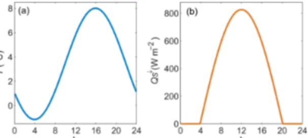
Figure 1.Idealized diurnal cycles of(a)temperature and(b) incom-ing shortwave radiation used in the energy balance model. These two examples are for a sample day, 1 July 2010, parameterized from daily minimum and maximum temperature in(a)and day of year plus mean daily incident shortwave radiation in(b).
content,
ρs=ρi(1−θ )+ρwθw+ρiθi, (16)
for porosity θ, liquid water fractionθw, and ice fractionθi.
Densities ρs, ρi, and ρw refer to snow, ice and water,
re-spectively. We prescribe a decrease in porosity with depth following θ (z)=0.6–0.05z, parameterized to represent the measured summer snow densities at the site (ρs=350–
550 kg m−3) and give reasonable estimates of firn density, up toρs=820 kg m−3at 10 m depth.
Snow accumulates, melts, or undergoes densification on a daily time step, with snow thicknessdvarying continuously (vs. discretely) within the fixed-grid framework. At depthd
below the surface, the grid cell has a weighted combination of thermal properties and densities to reflect the mixture of snow and either firn or ice in that layer. We do not have a model for snow accumulation through the winter months. We treat this simply and linearly accumulate snow from the start of winter until the start of the following melt season, with the accumulation rate set to give a match to the observed May snowpack thickness for each year. These data are available through annual winter mass balance surveys on the glacier, including a snow pit that provides depth and density mea-surements at the automatic weather station (AWS) site.
The steps in the energy balance and melt model are as fol-lows:
1. Daily mean values are input for temperature, incoming shortwave and longwave radiation, air pressure, specific humidity, wind speed, as well as minimum and maxi-mum temperature.
2. A diurnal temperature cycle is parameterized as a cosine wave with a lagτt=4 h to give the maximum tempera-ture at 16:00, as per local observations, with an ampli-tudeAt=(Tmax−Tmin)/2 (Fig. 1a). For timet(hour of
the day) and periodPt=24 h,
T (t )= −Atcos
2π (t−τt) Pt
. (17)
3. A diurnal cycle for incoming shortwave radiation is parameterized as a half-cosine wave with a period
Psw(d)=2hs(d), wheredis the day of year andhsis the
number of hours of sunlight on dayd(Fig. 1b). Defining lagτswand amplitudeAsw,
Q↓s(t )=max
−Aswcos
2π (t−τsw) Psw
,0
. (18) Sunlight hours are calculated as a function of latitude,
θ, and day of year, based on the equation for the sunset hourhss(e.g., Liou, 2002):
cos(hss)= −tan(δ)tan(θ ), (19)
whereδis the solar declination angle (solar latitude as a function of day of year). Sunlight hourshs=2hss. The
lag also varies with the day of year and is calculated by setting peak shortwave radiation to occur at noon: 2π(12−τsw)/Psw=π. This givesτsw=12−hshours.
AmplitudeAswis calculated by integrating the area
un-der the cosine curve and equating this to the average daily incoming shortwave radiation, Q↓Sd. This gives
Asw=12π Q↓Sd/hsW m−2. This treatment implicitly in-cludes cloud effects that reduce incoming shortwave ra-diation on a given day (viaQ↓Sd), but distributed evenly through the day. This neglects any systematic tendency for afternoon vs. morning clouds. For simplicity, we also neglect the effect of zenith angle on atmospheric transmittance (i.e., lower transmittance for larger atmo-spheric path lengths in the morning and late afternoon), although this could be built into a more refined model. 4. We assume that wind, incoming longwave radiation, air
pressure, and specific humidity are constant through the day, held to the mean daily value. For sensitivity tests,
Q↓L is calculated following Eq. (8) and the daily mean value ofQ↓S is perturbed from Eq. (10) anddQ↓S=dτ. 5. Relative humidity has a diurnal cycle following
temper-ature, assuming constant daily humidity but adjustingh
for consistency with the effect of temperature on satura-tion vapour pressure.
6. Albedo is also modelled on a daily basis for the sensi-tivity studies. When the seasonal snowpack is melted away, albedo is set to the observed bare-ice value at the site,αi=0.25. For fresh or dry snow, a fixed value
α0=0.86 is used. The snowpack thickness is initial-ized on 1 May of each year, set to the observed value measured during the annual winter mass balance survey. During the melt season, which is assumed to start after this date, seasonal snow albedo decreases as a function of cumulative positive degree days (P
PDD) following Hirose and Marshall (2013):
αs(d)=α0−kα
X
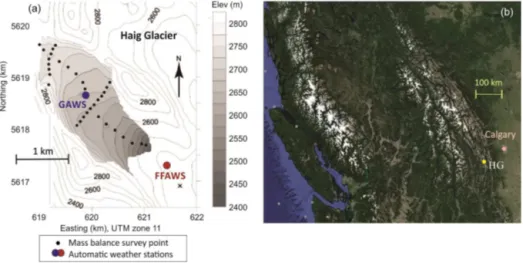
Figure 2. (a)The topography and automatic weather stations on Haig Glacier (GAWS) and the glacier forefield (FFAWS). The smaller black dots are mass balance survey points.(b)The location of Haig Glacier is labelled HG on the Google Earth map of southwestern Canada.
A minimum value of 0.4 is set for old snow. We pa-rameterize the effects of summer snowfall on albedo and mass balance through a stochastic model of sum-mer precipitation events (Marshall, 2014). Precipitation events are set to occur randomly, with 25 events occur-ring from May through September as the default set-ting. Precipitation totals vary randomly, between 1 and 10 mm w.e., with snow at temperatures below 0◦C, rain-fall above 2◦C, and rain/snow partitioning increasing linearly over the range 0–2◦C. Following a summer snow event, surface albedo is reset toα0, and its albedo
begins to decay following Eq. (20). This treatment al-lows a natural transition to end-of-summer conditions, when fresh snowfall in September or October does not melt away.
7. Subsurface temperatures and the conductive heat flux,
QC, are modelled with 10 min to 1 h time steps (cho-sen for stability of the temperature solution). The up-dated surface temperatureTsis used for the calculation of outgoing longwave radiation (Eq. 6), sensible heat flux (Eq. 11), and latent heat flux (viaqs in Eq. 12) for
the next time step.
8. The hydrology model calculates meltwater drainage and refreezing. Annual meltwater runoff is then the sum of all meltwater that drains, while summer mass balance is equal to the meltwater runoff minus the total summer snowfall, nominally for the period 1 May to 30 Septem-ber at this site. This allows for some meltwater retention as either liquid water or refrozen ice within the snow or firn. We neglect water storage in the englacial and sub-glacial hydrology systems.
3 Field site and observational data
Reference meteorological conditions, surface energy balance fluxes, and snow conditions are based on in situ measure-ments at Haig Glacier in the Canadian Rocky Mountains for the period 2002–2012 (Marshall, 2014). Winter mass balance measurements are carried out each May. These observations provide an 11-year record of observed snow depth and sum-mer melt from an AWS located near the median elevation of the glacier, 2660 m (Fig. 2). This is the upper ablation area of the glacier, which generally undergoes a transition from seasonal snow to exposed glacier ice in August.
Table 1 summarizes the mean observed meteorological and conditions at Haig Glacier over the 11-year reference period. Data coverage is incomplete, particularly in the win-ter months, as we transitioned to summer only measurements (May–September) after 2009. For the 11 years, data coverage is as follows for most sensors (e.g., temperature, shortwave radiation): JJA – 90 % (909 of 1012 days); MJJAS – 86 % (1441 of 1683 days); annual – 63 % (2519 of 4018 days). There are more missing longwave radiation data, as the sen-sor was not installed until July 2003. The corresponding numbers are JJA – 76 %; MJJAS – 70 %; annual – 46 %.
Missing data are gap-filled from a weather station that has operated continuously in the glacier forefield since 2001, at an elevation of 2325 m. The forefield AWS has more com-plete data coverage than the glacier AWS, above 90 % for all variables. Observational data are used to adjust for the altitudinal and environmental differences between the sites, through either a monthly offset (e.g.,TG=TFF−1T) or a
scaling factorβ(e.g.,vG=βvvFF). Here, subscriptsGandFF
con-Table 1. Mean monthly weather conditions±1 SD (standard deviation) at Haig Glacier, Canadian Rocky Mountains, May to Septem-ber 2002–2012. Data are from automatic weather station measurements at an elevation of 2660 m, in the upper ablation zone of the glacier.
Month T (◦C) h(%) ev(hPa) qv(g kg−1) P (hPa) v(m s−1)
May −1.4±1.1 73±4 4.0±0.4 3.4±0.4 743.0±2.4 2.8±0.2
June 2.6±0.9 73±6 5.5±0.5 4.6±0.4 748.1±1.4 2.6±0.2
July 6.9±1.4 62±5 6.4±0.4 5.3±0.3 751.2±1.6 2.8±0.3
August 5.9±1.1 64±7 6.1±0.4 5.1±0.4 750.8±1.4 2.5±0.2
September 2.1±1.8 71±10 5.0±0.4 4.2±0.3 748.4±1.8 3.0±0.4
JJA 5.1±0.8 67±4 5.7±0.4 4.8±0.3 750.0±1.1 2.6±0.2
MJJAS 3.2±0.7 69±4 5.3±0.3 4.3±0.3 748.3±1.4 2.7±0.2
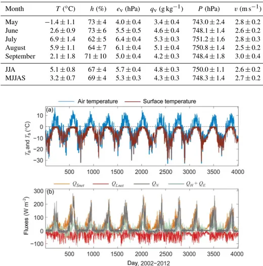
Figure 3.The 11-year record of(a)air temperature, modelled surface temperature, and(b)surface energy fluxes at the Haig Glacier AWS site. Daily mean values are plotted from 1 January 2002 to 31 December 2012.
sider only the point energy balance at the glacier AWS site. If both stations are missing data, gap-filling is done through assignment of mean daily observational data.
To give a sense of the complete data record, Fig. 3 shows examples of the full record, for air temperature, modelled surface temperature, and the energy fluxes. Average June to August (JJA) air and surface temperature are 5.1 and −0.6◦C, respectively, and 98 % of JJA days reach surface temperatures of 0◦C (melting conditions) in the 11-year record. The surface energy fluxes in Fig. 3b illustrate the dominance of net radiation in governing net energy at this site (Table 2).
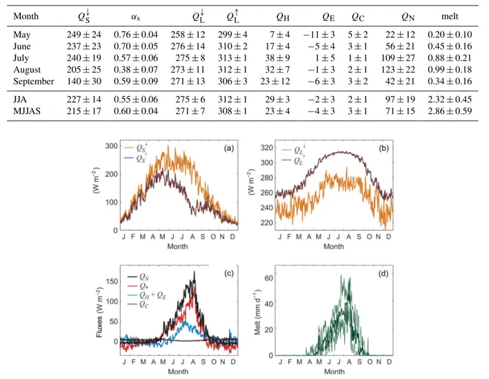
Mean daily values for the 11-year record are plotted in Fig. 4. As is typical for midlatitude glaciers, net radiation is the main energy flux that drives glacier melt at this site (Fig. 4c). Net radiation is negative in the winter, when short-wave inputs are low, albedo is high, and longshort-wave cooling gives a radiation deficit. Net radiation is positive in the sum-mer and increases through the melt season. This is driven
by increases in net shortwave radiation as snow albedo de-clines at the site and then melts away to expose the under-lying glacier ice (Fig. 4a). Measurements at the AWS site indicate a seasonal snow albedo decrease from about 0.8 to about 0.4 each summer, which may be due to a combina-tion of increased snow-water content, grain metamorphosis in the temperate snowpack, and increasing concentration of impurities through the melt season (e.g., Cuffey and Pater-son, 2010).
Table 2.Mean monthly surface energy balance terms±1 SD at Haig Glacier, Canadian Rocky Mountains, May to September 2002–2012. Radiation fluxes and albedo values are from automatic weather station measurements and the turbulent fluxes and subsurface heat conduction are modelled from the AWS data. Fluxes are in W m−2and melt totals are in m w.e.
Month Q↓S αs Q↓L Q↑L QH QE QC QN melt
May 249±24 0.76±0.04 258±12 299±4 7±4 −11±3 5±2 22±12 0.20±0.10
June 237±23 0.70±0.05 276±14 310±2 17±4 −5±4 3±1 56±21 0.45±0.16
July 240±19 0.57±0.06 275±8 313±1 38±9 1±5 1±1 109±27 0.88±0.21
August 205±25 0.38±0.07 273±11 312±1 32±7 −1±3 2±1 123±22 0.99±0.18
September 140±30 0.59±0.09 271±13 306±3 23±12 −6±3 3±2 42±21 0.34±0.16
JJA 227±14 0.55±0.06 275±6 312±1 29±3 −2±3 2±1 97±19 2.32±0.45
MJJAS 215±17 0.60±0.04 271±7 308±1 23±4 −4±3 3±1 71±15 2.86±0.59
Figure 4.The average annual cycle of(a–c)surface energy fluxes and(d)daily melt at the Haig Glacier AWS. Daily mean values are plotted for the period 2002–2012. For melt rates, the heavy line is the median value and the thin lines indicate the interquartile range.
The energy balance and snowpack models have been de-veloped and tested elsewhere (Marshall, 2014; Ebrahimi and Marshall, 2015), so we do not present the model validation in detail here. Comparisons are favourable between AWS observations (e.g., in situ albedo, SR50-inferred melt), the model driven with 30 min AWS data, and the “daily” version of the model used here, which includes parameterizations of albedo, incoming longwave radiation, and the diurnal tem-perature and shortwave radiation cycles (Sect. 2). The sim-plified daily model loses some reality, but its overall perfor-mance is excellent.
As an example, glacier AWS data from summer 2015 are used as an independent test of the model, with its de-fault parameterizations. Observed melt at the AWS site was 3.1±0.1 m w.e. in summer 2015, while the melt model forced by 30 min AWS data gives 3.04 m w.e. and the param-eterized, daily version of the model gives 2.98 m w.e. Tak-ing the 30 min AWS-driven results as the reference, the root
mean square error in the daily melt predictions for the param-eterized model is 3 % (0.7 mm w.e., relative to a daily mean value of 22.7 mm w.e.). Departures from the observations are primarily associated with the albedo, which is overestimated in summer 2015. Overall the parameterized daily model has good skill and is an appropriate tool for the sensitivity anal-yses presented here.
on summer melt at the Haig Glacier AWS site. Perturbations are introduced with respect to the mean JJA meteorological conditions from 2002 to 2012.
Theoretical sensitivities are calculated in this section by differentiating the net energy balance with respect to each meteorological variable. This is akin to generating a Jacobian matrix forQN, based on partial derivatives of the dependent
variables in the surface energy balance. One cannot gauge the most important meteorological influence on surface energy and mass balance from the sensitivities to a unit change in each variable. For instance, a change in specific humidity of 1 g kg−1equals 3.3 SD (standard deviations), with respect to the interannual (JJA) variability (Table 1). In contrast, sum-mer temperature has a standard deviation of 0.8◦C, so a 1◦C temperature change is a smaller perturbation. To allow a di-rect comparison of the theoretical sensitivities and to give a simple representation of their natural, interannual variability, we perturb each variable by 1 SD, based on the values re-ported in Tables 1 and 2.
We consider the core summer months, JJA, to calculate the theoretical sensitivity because the glacier surface is at melt-ing point for most of this time (Fig. 3a), which is a necessary condition to relate net energy to melt. More than 80 % of the annual melt also occurs in this season (Table 2 and Fig. 4d), so meteorological forcing over this period has the highest im-pact on glacier melt.
4.1 Sensitivity to temperature
Air temperature appears directly in the expressions forQ↓L
andQH. Temperature change may also influence the surface
energy balance through influences on other variables, such as atmospheric moisture (QE). For a melting glacier surface,
where surface and subsurface temperatures are at 0◦C, air temperature changes do not directly influenceQ↑LorQC. To estimate the magnitude of temperature sensitivity, we differ-entiate each energy balance flux with respect to temperature. For incoming longwave radiation, Eq. (7), the resulting temperature sensitivity is
∂Q↓L
∂T =4σ εaT 3 a +σ Ta4
∂εa
∂T. (21)
This general form applies to a range of formulations forεa, such as those of Brutsaert (1975), Lhomme et al. (2007), or Sedlar and Hock (2009). Adopting the parameterization in Eq. (8), which performs well at Haig Glacier, results in
∂Q↓L
∂T =4σ εaT 3 a +σ Ta4
b∂ev ∂T +c
∂h ∂T
. (22)
The last two terms reflect potential feedbacks of temperature change on humidity. While we are only considering pertur-bations to temperature in this section, vapour pressure and relative humidity cannot both remain constant under a tem-perature change. We first assume that relative humidity h
remains constant, under which conditions we assume that cloud cover and sky clearness will be unchanged. For con-stanth,ev scales with temperature following the Clausius–
Clapeyon relation for saturation vapour pressure:
∂ev ∂T = h 100 ∂es ∂T = h 100 L
ves RvTa2
= Lvev RvTa2
, (23)
where Rv=461.5 J kg−1◦C−1i s the gas-law constant for water vapour.
For the mean JJA meteorological conditions at Haig Glacier, Eqs. (22) and (23) give∂Q↓L/∂T=4.7 W m−2◦C−1. Temperature increases affectQ↓Lthrough both the direct ef-fect of higher emission temperatures and the indirect efef-fect of higher atmospheric emissivity, with these two terms in Eq. (21) contributing 4.0 and 0.7 W m−2◦C−1, respectively.
The temperature sensitivity of sensible and latent heat fluxes follow
∂QH ∂T =
ρacpk2v
ln(z/z0)ln z/z0H
(24)
and
∂QE
∂T =
ρaLpk2v
ln(z/z0)ln z/z0E
∂q v ∂T , (25) where ∂qv ∂T ≈ Rd P Rv
∂e
v ∂T
(26)
for the dry gas-law constant Rd=289 J kg−1◦C−1 and air
pressureP, under the assumption that air pressure and den-sity are constant for small changes in temperature. Table 3 gives the turbulent flux sensitivities for mean JJA conditions at Haig Glacier. Perturbations to bothQHandQEare
pos-itive with an increase in temperature and the assumption of constanth. In combination with the increase inQ↓L, net en-ergy over the summer months is augmented by 12 W m−2 for a 1◦C increase in temperature. Interannual variations in summer temperature (1σ) equal 0.8◦C, giving a net energy perturbationδQNσ= +10 W m−2(Table 3).
Fluctuations in energy balance can be related to melt rates through their combined influence on QN, with
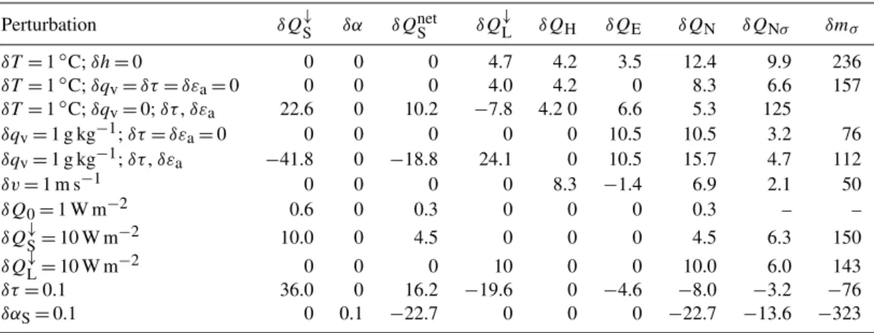
Table 3. Surface energy balance sensitivity to meteorological perturbations over a melting glacier surface, from direct feedbacks only. Calculations are for mean JJA conditions at Haig Glacier. All energy flux perturbations are expressed in W m−2.δQNσ is the net energy
perturbation for a 1σincrease in the variable. The melt perturbation,δmσ, has units of mm w.e. and is calculated assuming thatδQNσ holds
for JJA (92 days).
Perturbation δQ↓S δα δQnetS δQL↓ δQH δQE δQN δQNσ δmσ
δT=1◦C;δh=0 0 0 0 4.7 4.2 3.5 12.4 9.9 236
δT=1◦C;δqv=δτ=δεa=0 0 0 0 4.0 4.2 0 8.3 6.6 157
δT=1◦C;δqv=0;δτ,δεa 22.6 0 10.2 −7.8 4.2 0 6.6 5.3 125
δqv=1 g kg−1;δτ=δεa=0 0 0 0 0 0 10.5 10.5 3.2 76
δqv=1 g kg−1;δτ,δεa −41.8 0 −18.8 24.1 0 10.5 15.7 4.7 112
δv=1 m s−1 0 0 0 0 8.3 −1.4 6.9 2.1 50
δQ0=1 W m−2 0.6 0 0.3 0 0 0 0.3 – –
δQ↓S=10 W m−2 10.0 0 4.5 0 0 0 4.5 6.3 150
δQ↓L=10 W m−2 0 0 0 10 0 0 10.0 6.0 143
δτ=0.1 36.0 0 16.2 −19.6 0 −4.6 −8.0 −3.2 −76
δαS=0.1 0 0.1 −22.7 0 0 0 −22.7 −13.6 −323
melt provide an intuitive way to understand and compare sen-sitivities. We consider more realistic relations between net energy and melt in the modelled sensitivities of Sect. 5.
This initial scenario assumes that the warmer atmosphere contains more moisture, which is not necessarily the case. For instance, high summer temperatures in this region are commonly associated with ridging and subsidence, i.e., hot, dry conditions. If we assume thatqvis invariant with
temper-ature (case 2 in Table 3), there is no feedback on the latent heat flux and the increase in net energy is less than with con-stanth:δQNσ=6.6 W m−2andδmσ=157 mm w.e.
However, there are additional feedbacks associated with relative humidity. If qv is invariant, relative humidity must change to be consistent with the temperature perturbation. As an example, an increase of 1◦C with no change inqv corre-sponds to a decrease of 6 % in mean summerhat our site, to 61 %. This lowers the atmospheric emissivity in Eq. (8), re-duces the incoming longwave radiation, and impacts∂εa/∂T
in Eq. (22). To be internally consistent, reduced humidity anomalies should also be associated with changes in cloud cover. For the 1◦C temperature increase, the 6 % decrease in relative humidity corresponds to an increase in clearness index of 0.06 (Eq. 10) from 0.63 to 0.69.
The effects of these radiation feedbacks are given in Ta-ble 3. Reduced relative humidity decreasesQ↓Land increases
Q↓S. The resulting increase in shortwave radiation partially offsets the decline in Q↓L, but there is an overall reduction in net radiation. For our parameterizations of the incom-ing radiation fluxes as a function of humidity, the effect of drier air on longwave radiation is stronger than the short-wave radiation feedback. This reduces the overall sensitiv-ity to temperature change relative to the first two cases, with
δQNσ=5.3 W m−2andδmσ=125 mm w.e. Note that these temperature scenarios are all idealized, neglecting albedo
feedbacks and other indirect effects of a temperature change. These feedbacks are assessed in Sect. 5.
4.2 Sensitivity to humidity and wind
Similar derivatives and energy balance sensitivities can be derived with respect to the other meteorological variables to explore the sensitivity of summer melt to different weather conditions. The sensitivity of sensible and latent heat fluxes to wind perturbations follow
∂QH ∂v =
ρacpk2(Ta−Ts)
ln(z/z0)ln z/z0H
(27)
and
∂QE
∂v =
ρaLpk2(qv−qs)
ln(z/z0)ln z/z0E
, (28)
while the sensitivity to humidity is
∂QE
∂qv =
ρaLpk2v
ln(z/z0)ln z/z0E
. (29)
Incoming longwave radiation is also affected by perturba-tions in humidity, following
∂Q↓L
∂qv =σ T 4 a
∂εa
∂qv=σ T 4 a
b∂ev ∂qv+c
∂h
∂qv
. (30)
Changes in humidity directly impact the latent heat flux and may also influence incoming longwave radiation and cloud cover (hence, incoming shortwave radiation). We consider the effects of a humidity perturbation with and without radiative feedbacks in Table 3. For δqv=1 g kg−1
and fixed temperature, mean summer relative humidity in-creases by 12, to 79 %, and QE and QN increase by
10.5 W m−2. Interannual variations in qv equal 0.3 g kg−1,
givingδQNσ=3.2 W m−2, corresponding to a 76 mm (3 %) increase in summer melt.
Where radiation feedbacks are included, the increases in specific and relative humidity have a strong influence on the atmospheric emissivity in Eq. (8), giving an increase inQ↓L
of 24 W m−2. This is partially offset by cloud feedbacks as-sociated with the increased humidity. Following Eq. (10),
δh=12 % equates to a decrease in atmospheric transmissiv-ity of 0.11, which strongly attenuates incoming shortwave ra-diation. This reduces the net radiation by 19 W m−2, but the radiation feedbacks remain positive. The net impact of a 1σ
humidity perturbation δqv=0.3 g kg−1 is then 4.7 W m−2,
corresponding to a 112 mm (5 %) increase in summer melt. Wind perturbations have straightforward linear effects on QH and QE, giving a net sensitivity ∂QN/∂v= +7 W m−2(m s−1)−1. Sensible heat flux
in-creases and evaporative cooling dein-creases slightly. Winds have a low interannual variability at this site, 0.2 m s−1, so the associated net energy anomaly is δQNσ=2 W m−2, equivalent to 50 mm w.e. in summer melt.
4.3 Sensitivity to the radiation fluxes
Net shortwave radiation is affected by variations in top-of-atmosphere insolation, the clearness index (i.e., cloud condi-tions), and surface albedo. Our functional relationship for net shortwave radiation isQSnet=Q
↓
S(1−αS)=QSϕτ (1−αS), for potential direct insolation QSϕ and clearness index τ. From Eq. (4), sensitivity to top-of-atmosphere insolationQ0
follows
∂QSnet
∂Q0
=τ (1−αS)cos(Z)ϕP /P0cos(Z)
0 . (31)
An anomaly of 1 W m−2 in the top-of-atmosphere insola-tion,Q0, givesδQ↓S=0.6 W m−2, and the net radiation
im-pact is further reduced to 0.3 W m−2by the surface albedo. The net impact of top-of-atmosphere solar variability, such as sunspot cycles, is therefore small.
In contrast, incoming radiation fluxes and energy balance are strongly sensitive to atmospheric transmissivity, which in turn is largely governed by cloud cover. Direct, independent variations in incoming shortwave and longwave radiation are reported in Table 3 for fluctuations of 10 W m−2and for 1σ
variations in each. Sensitivity is moderate, of order 6 % of the net energy.
It is more appropriate to consider covariations of these radiation fluxes that can be expected in association with
changes in cloud cover. We can estimate through the sky clearness index,τ, as parameterized via Eqs. (9) and (10), which relate the atmospheric emissivity and relative humid-ity to clearness index. As an example, reduced cloud cover may be associated with a 1σ increase inτ of 0.1, from 0.63 to 0.73. This translates to an increase in net shortwave en-ergy of 16 W m−2 (Table 3), but the change in cloud cover also impacts incoming longwave radiation. Clearer skies in the example of Table 3 give lowerh, lowerev, and lowerQ↓L.
Latent heat flux also declines. The overall result is a reduc-tion in net energy for an increase inτ. A 1σincrease (+0.04) gives a 3 % reduction in net energy.
4.4 Sensitivity to albedo
The sensitivity to albedo changes is comparatively high. An change in albedo of 0.1 creates an energy balance perturba-tion of more than 100 W m−2at local noon in mid-summer. The magnitude of this effect varies with latitude, time of year, and atmospheric transmissivity. Integrated over the daily so-lar path and over the summer, an albedo increase of 0.1 re-duces net solar radiation by−23 W m−2. Measurements at the site indicate an interannual albedo variability of 0.06, equivalent to 14 % of the net energy orδmσ= −323 mm w.e. 4.5 Summary
Overall, the results indicate a strong sensitivity of the sum-mer energy balance and melt to temperature and albedo, with weaker influences from cloud conditions, humidity, and wind speed.
These theoretical sensitivities are idealized, however, and neglect many important feedbacks and glaciometeorologi-cal interactions that occur in glacier environments. The next two sections examine the energy balance sensitivity at Haig Glacier within an energy-balance melt model. This allows an estimate of feedbacks associated with the evolution of albedo, interannual variability in weather conditions, and meteorologically consistent covariance of weather variables.
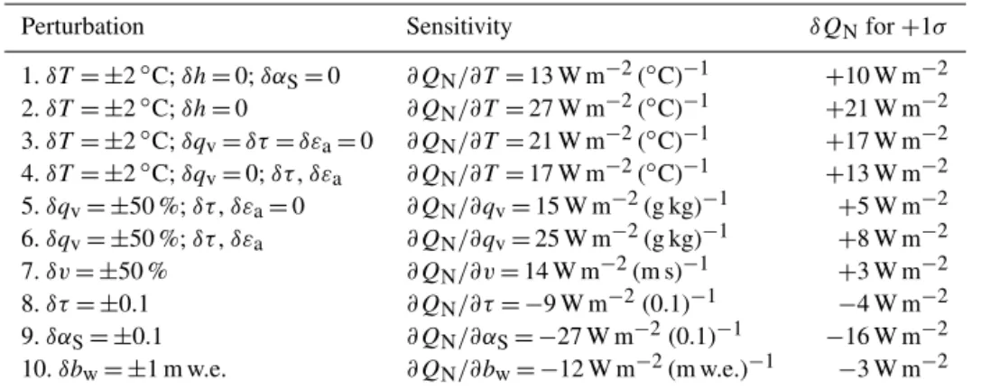
Table 4.Net energy balance sensitivity to meteorological perturbations in the surface energy balance model, based on regressions to the sensitivity curves (cf. Fig. 6). Also shown is the change in net energy associated with a 1σincrease in each parameter, averaged over JJA.
Perturbation Sensitivity δQNfor+1σ
1.δT= ±2◦C;δh=0;δαS=0 ∂QN/∂T=13 W m−2(◦C)−1 +10 W m−2
2.δT= ±2◦C;δh=0 ∂QN/∂T=27 W m−2(◦C)−1 +21 W m−2
3.δT= ±2◦C;δqv=δτ=δεa=0 ∂QN/∂T=21 W m−2(◦C)−1 +17 W m−2
4.δT= ±2◦C;δqv=0;δτ,δεa ∂QN/∂T=17 W m−2(◦C)−1 +13 W m−2
5.δqv= ±50 %;δτ,δεa=0 ∂QN/∂qv=15 W m−2(g kg)−1 +5 W m−2
6.δqv= ±50 %;δτ,δεa ∂QN/∂qv=25 W m−2(g kg)−1 +8 W m−2
7.δv= ±50 % ∂QN/∂v=14 W m−2(m s)−1 +3 W m−2
8.δτ= ±0.1 ∂QN/∂τ= −9 W m−2(0.1)−1 −4 W m−2
9.δαS= ±0.1 ∂QN/∂αS= −27 W m−2(0.1)−1 −16 W m−2
10.δbw= ±1 m w.e. ∂QN/∂bw= −12 W m−2(m w.e.)−1 −3 W m−2
Perturbations to the observed weather are used to repeat the sensitivity analyses of Sect. 4, but with a realistic evo-lution of each summer melt season rather than the mean summer conditions. Meteorological variables are perturbed as follows: ±2◦C for temperature,±50 % for specific hu-midity and wind,±0.1 for the sky clearness index (a proxy for cloud cover), and±0.1 for albedo. Increments are set to give 41 realizations in each case, spanning the range of the perturbation. For example, temperature increments of 0.1◦C are applied for the range −2 to 2◦C. Each perturbation is prescribed for all days in the original data, and the energy balance program is run for the period 2002–2012. In each experiment, all other meteorological variables are held con-stant except for those that are direct impacted by a perturba-tion (e.g., relative humidity changes with temperature).
Table 4 lists the response of mean summer (JJA) net energy, QN, to the different meteorological perturbations.
Changes in the energy fluxes can be examined in response to the perturbations, e.g.,1QNas a function of temperature
anomalies,δT. We plot these values to give sensitivity curves (e.g., Figs. 5 and 6), and the slope of each curve is a mea-sure of the sensitivity, e.g., dQN/dT. Values in Table 4 are
calculated through linear regression. The relationship area is generally nonlinear, so we compute the regressions for the region of the sensitivity curve within ±1 SD (±1σ) of the reference value for each variable. This samples a more linear range and allows a better comparison with the derivatives in Table 3. Standard deviations refer to the interannual variabil-ity, as reported in Table 1. Table 4 also lists the change in net energy associated with a 1σ increase in each variable.
There are multiple scenarios for temperature, shown in the first four cases in Table 4. These cases represent different assumptions about the way in which atmospheric moisture and radiation fluxes respond to a temperature perturbation. The first two cases follow the assumption that relative hu-midity does not change. Hence, a temperature change δT
is attended by a change in specific humidity,δqv, to
main-tain constanth. This impacts latent heat flux and atmospheric
Figure 5.Sensitivity of modelled summer (JJA) melt to temper-ature perturbations for different assumptions, as per Table 4. The reference (mean 2002–2012) JJA melt is 2.32 m w.e.
emissivity. Cases 1 and 2 show the net energy sensitivity to this scenario without and with albedo feedbacks. The next two cases include albedo feedbacks but assume no change in specific humidity,δqv=0; hence relative humidity must
respond. Cases 3 and 4 are without and with atmospheric ra-diation feedbacks to the changed relative humidity.
Summer melt sensitivity for the four different tempera-ture perturbation scenarios is plotted in Fig. 5. Case 1 lacks albedo feedbacks and corresponds to a net energy sensitiv-ity of 13 W m−2◦C−1, which is comparable to the theoreti-cal temperature sensitivities in Table 3. This is due to direct temperature/humidity impacts on incoming radiation fluxes, sensible heat flux, and latent heat flux. Cases 2–4 include albedo feedbacks. This can be considered to be more realis-tic, and the albedo feedbacks have a roughly 2-fold ampli-fication effect on the temperature perturbation. Under con-stanth, dQN/dT=27 W m−2◦C−1 (cf. Fig. 6a),
represent-ing a 28 % increase in summer melt for a 1◦C warming. This decreases by 6–10 W m−2◦C−1in cases 3 and 4, whereqv
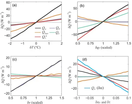
at-Figure 6.Sensitivity of the surface energy fluxes at Haig Glacier to changes in(a)temperature (case 2),(b)specific humidity (case 6),
(c)wind speed (case 7), and(d)atmospheric transmittance (case 8) and albedo (blue line, case 9). All lines are anomalies relative to the baseline data from the period 2002–2012, and they indicate the mean sensitivity of the different energy fluxes over this period. Please note the differenty(δQ)scales.
mospheric radiation feedbacks, reduces energy further as de-creased cloud cover (via higher τ) reduces incoming long-wave radiation more strongly than it increases shortlong-wave fluxes in the model. Here, too, the numerical model gives a similar result to the theoretical prediction.
Figure 6a plots the response of the different surface en-ergy fluxes for the reference model, case 2. Net shortwave radiation dominates the temperature response, overQH,QE, andQ↓L. Figure 6b–d provide similar details for perturbations in humidity, wind, clearness index, and albedo (cases 5–9 in Table 4). Sensitivity to humidity changes is relatively strong, through the combined impacts of latent and longwave fluxes (Fig. 6b). Case 6 is shown in this figure, including feedbacks on the atmospheric radiation. Incoming longwave radiation is strongly augmented by the increases in absolute and rela-tive humidity and accounts for about 70 % of the net energy sensitivity to specific humidity. It is partially offset by cloud feedbacks, however, which reduce incoming shortwave radi-ation.
For increases in both temperature and humidity, the mean summer latent heat flux switches sign from negative (Table 2) to positive; that is, latent heat flux becomes a source rather than sink of energy under warmer and wetter conditions. In contrast, latent heat flux remains negative, but small, under increases in wind speed (Fig. 6c). Energy balance sensitivity to wind perturbations is primarily associated with the sensi-ble heat flux.
Net energy perturbations due to albedo and clearness in-dex in Fig. 6d are independent of each other, but they are
plotted together for convenience. Albedo sensitivity over the range±0.1 is relatively high, with a decrease in net energy of 27 W m−2(28 %) for an increase in albedo of 0.1. Changes in sky clearness index (atmospheric transmissivity) have a lower impact due to the compensating influences on incom-ing shortwave and longwave radiation. Reduced cloud cover (higherτ) gives an overall reduction in net energy at our site, as longwave radiation effects are dominant.
Sensitivity to winter snow accumulation
Changes in the winter mass balance also influence the sum-mer melt season. Interannual variability in the amount of snow is implicit in the simulations, as the spring (1 May) snowpack depth is initialized with the measured winter mass balance for each year,bw (Marshall, 2014). However, these experiments do not control for the influence of snow depth on summer melt extent.
To examine this, we force the energy balance model over a range of winter mass balance conditions,
bw∈[0.36, 2.36] m w.e. This is ±1 m w.e. relative to
which become more frequent as temperatures cool in September.
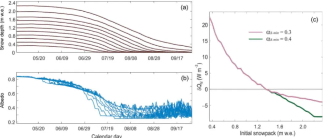
The net energy balance perturbations that accompany these scenarios are shown for two choices of the minimum snow albedo (Fig. 7c). Observations of late-summer snow at the site are in the range 0.3–0.4, the two values presented here. The plot is asymmetric: net energy is more sensitive to reduced winter snow depths, which result in an earlier transi-tion to exposed glacier ice. A 20 % (1σ) reduction inbwgives
a net energy increase of about 4 W m−2(4 %), and the sen-sitivity increases nonlinearly with increasingly lower snow depths. The influence from a deep winter snowpack is com-paratively muted: 1–2 W m−2 reductions inQN for a 20 % increase in the winter snow thickness. Perturbations inQN
asymptote once seasonal snow is deep enough to survive through the summer.
The influence of the winter snowpack at this site is similar in magnitude to the net energy impacts of interannual varia-tions in wind speed but less important to the summer melt than observed variations in temperature, albedo, or cloud cover. This result is partly due to the relatively low contrast between late-summer snow albedo and bare-ice albedo at this site. If late-summer snow has a higher albedo, a deep win-ter snowpack is more effective at reducing the net energy and summer melt. The shape of the sensitivity curve would change for locations with higher-albedo snow as well as for sites in the lower ablation zone, where ice is exposed early in the melt season. A heavy winter snowpack would have a comparatively stronger role in this case. The result in Fig. 7 is therefore more site specific than for the other meteorological perturbations.
6 NARR-based surface energy balance reconstructions, 1979–2014
To examine energy balance sensitivity over a longer time pe-riod and with joint variation in meteorological variables, we run the energy balance model forced by NARR atmospheric reconstructions from 1979 to 2014 (Mesinger et al., 2006). This provides a more complete picture of interannual vari-ability, while comparison of NARR predictions with mea-surements over the period 2002–2012 also allows us to as-sess the skill with which fluctuations in surface energy bal-ance and summer melt can be captured in an atmospheric model that does not explicitly resolve the alpine and glacier conditions.
We use a perturbation approach as in Sect. 5, taking NARR daily meteorological fields as anomalies relative to the mean NARR conditions for the period 2002–2012. Anomalies in near-surface temperature, specific humidity, wind speed, pressure, incoming shortwave radiation, and incoming long-wave radiation are used to drive the model for the 36-year period 1979–2014. Perturbations are introduced as anoma-lies relative to the mean observed conditions. NARR input
fields allow us to introduce multiple perturbations at once, with magnitudes that are physically meaningful and meteo-rologically consistent covariance of variables.
NARR has an effective spatial resolution of 32 km, and we extract mean daily data from the grid cell over Haig Glacier. This grid cell has an elevation of 2214 m, about 450 m lower than the AWS site. By using daily weather anomalies, we avoid most biases associated with the different altitude of the NARR grid cell. However, variations in some fields such as specific humidity, pressure, and temperature can be larger at lower elevations and over non-glacierized land surface types. Since we use meteorological fluctuations as perturbations, this is potentially problematic. Inspection of the summer variance in the different meteorological inputs over the refer-ence period 2002–2012 indicates that this does not appear to be an issue. Standard deviations of each variable, calculated from mean JJA values, are as follows: temperature, 0.8◦C; specific humidity, 0.2 g kg−1; wind speed, 0.3 m s−1; incom-ing shortwave radiation, 6 W m−2; and incoming longwave radiation, 3 W m−2. Temperature, humidity, and wind values are equivalent to the observed range of variability from 2002 to 2012 (Table 1), but the radiation fluxes are less variable. The effects of a lower elevation in the NARR grid cell appear to be less than those associated with systematic biases in the reanalysis, e.g., not enough variability in cloud conditions.
The energy balance model requires an estimate of win-ter snow accumulation. We base this on cumulative NARR precipitation for the period September to May of each year, normalized to the observed value of 1.36 m w.e. at the Haig Glacier AWS site. This permits interannual variability in the winter snowpack thickness to be included in the simulations by scaling the mean observed value up or down based on the NARR winter precipitation totals. We use this as an initial condition for the melt model (i.e., for 1 May snow depth).
We examine the sensitivity of net summer energy balance and melt to interannual variations in each weather variable in the NARR forcing. Table 5 reports the NARR-based surface energy fluxes and melt for JJA and MJJAS, averaged over the period 1979–2014. Mean values are all within 2 W m−2 of the reference surface energy fluxes (Table 2), derived from the in situ data, but there are some significant differences in the standard deviation, which is a measure of the interan-nual variability. As noted above, incoming shortwave radia-tion has about half of the variability in the 36-year NARR record as observed in the 11-year measurement period, and variance in incoming longwave radiation is also less than ob-served. This implies more uniform summer cloud conditions in the reanalysis compared to the observational period.
end-of-Figure 7.Sensitivity to the winter mass balance, examined by varying 1 May snow depth from 0.36 to 2.36 m w.e., relative to the reference value of 1.36 m w.e. at the glacier AWS. (a)Snow depth and(b)albedo through the summer melt season, 1 May–30 September, for the different initial snow depths.(c)Net summer (JJA) energy balance change as a function of the winter mass balance for two different settings of the minimum snow albedo.
Table 5.Summer surface energy balance fluxes on Haig Glacier as forced by the North American Regional Reanalysis (NARR) daily weather fields, 1979–2014. NARR inputs are taken as perturbations to the mean observed values. Melt is in m w.e., and all fluxes have unit W m−2.
Period Q↓S αs Q↓L Q
↑
L QH QE QC QN Melt
JJA 227±7 0.53±0.05 275±4 311±1 27±4 −3±3 2±1 95±14 2.28±0.42
MJJAS 215±6 0.55±0.04 271±4 308±2 22±3 −5±3 3±1 73±10 2.68±0.50
summer to the winter accumulation season. This transition occurs sometime in September or October each year in our study period. September is mixed on the glacier, with fresh snowfall alternating with periods of melting. This raises the average albedo on the glacier, but our albedo parameteriza-tion does not fully capture this.
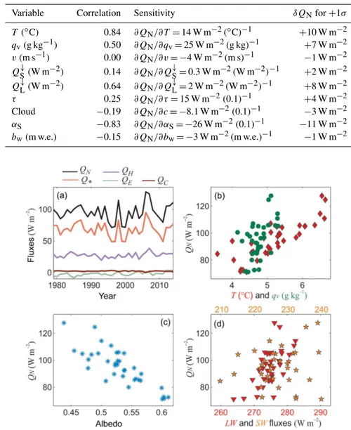
Figure 8a plots time series of the NARR-forced surface en-ergy balance terms, and Fig. 8b–d show the relations between net energy and selected meteorological variables. These pro-vide a visual indication of the strength of each variable as a predictor of summer melt. Regressions through these data points give estimates of net energy sensitivity, e.g.,∂QN/∂T,
as seen in actual realizations of the summer weather condi-tions. These gradients can be thought of as the melt sensitiv-ity to interannual variabilsensitiv-ity or trends in each weather vari-able.
The resulting sensitivities are given in Table 6, as well as linear correlation coefficients betweenQNand all
glaciome-teorological variables that are used in the energy balance model. These simulations are forced with NARR radiation flux anomalies, so we do not parameterize the incoming long-wave or shortlong-wave radiation in these tests. The clearness in-dex,τ, is not used, but it can be calculated from the NARR relative humidity estimate, via Eq. (10), or more directly through the fraction of incoming shortwave radiation relative to the clear-sky potential radiation. We test both approaches and find similar results. Values for∂QN/∂τ reported in
Ta-ble 6 are averaged from the two approaches. We also report
the direct relation between NARR total cloud cover and net energy; cloud cover is available in the reanalysis, but we do not have in situ data to compare with.
Temperature and albedo have the strongest influences on summer energy balance and melt. Fluctuations in specific humidity and incoming longwave radiation also correlate strongly with interannual variability in the summer energy budget. Wind speed, cloud conditions, and incoming short-wave radiation do not strongly contribute to the year-to-year variations in summer melt over the NARR period. There is a weak, positive relationship between the clearness index and net radiation in the NARR-forced results, indicating that in-creased shortwave radiation associated with reduced cloud cover has a stronger role than the associated reduction in longwave radiation.
Table 6.Correlation and sensitivity of different weather variables to the mean summer (JJA) net energy flux,QN, for the NARR simulations,
1979–2014. “Cloud” is the NARR total cloud fraction.
Variable Correlation Sensitivity δQNfor+1σ
T (◦C) 0.84 ∂QN/∂T=14 W m−2(◦C)−1 +10 W m−2
qv(g kg−1) 0.50 ∂QN/∂qv=25 W m−2(g kg)−1 +7 W m−2
v(m s−1) 0.00 ∂QN/∂v= −4 W m−2(m s)−1 −1 W m−2
Q↓S(W m−2) 0.14 ∂QN/∂Q↓S=0.3 W m−2(W m−2)−1 +2 W m−2 Q↓L(W m−2) 0.64 ∂QN/∂Q↓L=2 W m−2(W m−2)−1 +8 W m−2
τ 0.25 ∂QN/∂τ=15 W m−2(0.1)−1 +4 W m−2
Cloud −0.19 ∂QN/∂c= −8.1 W m−2(0.1)−1 −3 W m−2
αS −0.83 ∂QN/∂αS= −26 W m−2(0.1)−1 −11 W m−2
bw(m w.e.) −0.15 ∂QN/∂bw= −3 W m−2(m w.e.)−1 −1 W m−2
Figure 8. (a Mean summer (JJA) NARR-forced surface energy fluxes at Haig Glacier, 1979–2014. Mean summer net energy as a function of (b)temperature and specific humidity,(c)albedo, and(d)incoming shortwave and longwave radiation. Table 6 gives the associated correlations.
results (Tables 3 and 4), which are based on the in situ data. The largest exception is the relation between clearness index (cloud cover) and net energy, which is opposite in sign.
7 Discussion
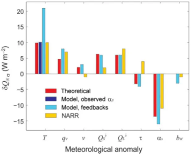
We have taken three different approaches to estimate sum-mer (JJA) energy balance and melt sensitivity at Haig Glacier: (i) theoretical, perturbing one variable at a time; (ii) a numerical model, restricting model experiments to sin-gle perturbations but allowing for internal feedbacks to be modelled; and (iii) through perturbations from a regional climate reanalysis, allowing multiple variables to change at
once. Here we briefly summarize and interpret the integrated results from these different methods.
7.1 Haig Glacier energy balance sensitivities and feedbacks
Figure 9.Net energy sensitivity to a 1σ perturbation in different meteorological variables: comparison of theoretical, in situ numeri-cal model, and NARR-based estimates.
Temperature changes are generally thought of as the main driver of glacier advance and retreat, through combined influences on the surface energy budget, snow accumula-tion, and summer melt season. Sensitivities to tempera-ture are commonly expressed as the change in summer or net mass balance per unit warming. Sample mass balance sensitivities reported in the literature are −0.6 m w.e.◦C−1 on Morteratschgletscher, Switzerland (Klok and Oerlemans, 2004), and Illecillewaet Glacier, British Columbia (Hirose and Marshall, 2013), −0.68±0.05 m w.e.◦C−1 for a suite of glaciers in Switzerland (Huss and Fischer, 2016), and −0.86 m w.e.◦C−1 on South Cascade Glacier, Washington (Anslow et al., 2008). Values as high as −2.0 m w.e.◦C−1 are reported for Brewster Glacier, New Zealand (Anderson et al., 2010).
These values are for the annual mass balance, but they are dominated by the summer melt response to warming. They represent a melt sensitivity of about 30 %◦C−1for the exam-ples in the Alps and western North America. When we intro-duce temperature perturbations in the absence of albedo feed-backs, we find a relatively muted energy balance response, about 13 %◦C−1. The increase in net energy is distributed about equally across the sensible heat flux, incoming long-wave radiation, and latent heat flux, and we have similar re-sults for both the theoretical and numerically modelled tem-perature perturbations. Albedo feedbacks increase the net en-ergy sensitivity to 28 %◦C−1 or −0.66 m w.e.◦C−1, in ac-cord with previous studies. The exact number depends on assumptions about humidity; if specific humidity increases with temperature (e.g., by holding relative humidity con-stant), temperature sensitivity is higher.
The albedo feedback results from two main ways that tem-perature influences the seasonal albedo evolution. A more in-tense melt season gives rise to a lower snow albedo and an earlier transition from seasonal snow cover to glacial ice. We do not explicitly model impurities or snow albedo processes
(e.g., grain metamorphosis, effects of snow-water content on the albedo), but we parameterize the seasonal albedo evolu-tion as a funcevolu-tion of cumulative PDD (Eq. 20), which makes the model directly sensitive to temperature perturbations.
Temperature changes have several additional, indirect im-pacts, including (i) a longer melt season, (ii) a greater fraction of time with surface temperatures at the melting point dur-ing the year, i.e., with reduced overnight cooldur-ing and refreez-ing, and (iii) an increase in the frequency of summer rain vs. snow events. Summer snow events have an important impact on surface albedo, with fresh snow strongly attenuating melt. Each of these processes contributes to the strong impact of temperature anomalies on glacier melt. Combined with the albedo feedbacks, these processes and help to explain why glaciers are strongly sensitive to temperature change.
Direct changes to albedo have an influence on summer en-ergy balance and melt extent that is comparable to the tem-perature influence,∼17 % for a change in albedo equal to the interannual albedo fluctuations, 0.06. Mean summer albedo differences arise as a feedback to other meteorological forc-ings that drive the summer snow melt, but interannual albedo variations also occur more directly, as a consequence of sum-mer snowfall events, as a function of winter accumulation totals, or due to impurity loading (e.g., black carbon deposi-tion). The latter has been observed in association with forest fires in British Columbia. Strong fire seasons occurred twice during our period of study, in 2003 and 2015, and each left a measurably darker glacier surface. For instance, the average albedo recorded at the AWS site in August 2003 was 0.13.
We found a relatively weak influence of winter mass bal-ance on the summer melt extent. A low snowpack depth has a greater impact, through an earlier transition to low-albedo bare ice. A deep winter snowpack has the opposite influence, supporting a higher average summer albedo, but the influ-ence is weaker because the AWS site is in the upper ablation area, where the seasonal snowpack persists until late sum-mer in most years. The effects of greater winter accumulation plateau once there is enough snow to survive the summer; beyond this point, additional snow has no effect on the sum-mer albedo or melt extent. Sensitivity to winter mass balance would likely be stronger at lower altitudes on the glacier and for the overall glacier mass balance.
Humidity changes can also be considered a feedback to temperature, but this is not certain; specific humidity varies as a function of local- to synoptic-scale moisture sources and weather patterns, and these are not necessarily cou-pled to temperature conditions. For instance, warm condi-tions at Haig Glacier often accompany anticyclonic ridging in the summer months, during which time southerly flows and upper-level subsidence promote dry, clear-sky condi-tions (lowqv andh). At other times, westerly flows bring