Processes governing the mass balance of Chhota Shigri Glacier (Western Himalaya, India) assessed by point-scale surface energy balance measurements

(1)

TCD

8, 2867–2922, 2014

Processes governing the mass balance of Chhota Shigri Glacier

(Western Himalaya, India)

M. F. Azam et al.

Title Page

Abstract Introduction

Conclusions References

Tables Figures

◭ ◮

Back Close

Full Screen / Esc

Printer-friendly Version

Interactive Discussion

Discussion

P

a

per

|

Discus

sion

P

a

per

|

Discussion

P

a

per

|

Discussion

P

a

per

|

The Cryosphere Discuss., 8, 2867–2922, 2014 www.the-cryosphere-discuss.net/8/2867/2014/ doi:10.5194/tcd-8-2867-2014

This discussion paper is/has been under review for the journal The Cryosphere (TC). Please refer to the corresponding final paper in TC if available.

Processes governing the mass balance of

Chhota Shigri Glacier (Western Himalaya,

India) assessed by point-scale surface

energy balance measurements

M. F. Azam1,2, P. Wagnon1,3, C. Vincent4, AL. Ramanathan2, A. Mandal2, and J. G. Pottakkal2

1

IRD/UJF – Grenoble I/CNRS/G-INP, LGGE UMR 5183, LTHE UMR 5564, 38402 Grenoble Cedex, France

2

School of Environmental Sciences, Jawaharlal Nehru University, New Delhi 110067, India

3

ICIMOD, GP.O. Box 3226, Kathmandu, Nepal

4

UJF – Grenoble I/CNRS, LGGE UMR 5183, 38041 Grenoble Cedex, France

Received: 26 April 2014 – Accepted: 20 May 2014 – Published: 5 June 2014 Correspondence to: M. F. Azam (farooqaman@yahoo.co.in,

farooq.azam@lgge.obs.ujf-grenoble.fr)

(2)

TCD

8, 2867–2922, 2014

M. F. Azam et al.

Title Page

Tables Figures

◭ ◮

Back Close

Full Screen / Esc

Discussion

P

a

per

|

Discus

sion

P

a

per

|

Discussion

P

a

per

|

Discussion

P

a

per

|

Abstract

Recent studies revealed that Himalayan glaciers have been shrinking at an accelerated rate since the beginning of the 21st century. However the climatic causes for this shrink-age remain unclear given that surface energy balance studies are almost nonexistent in this region. In this study, a point-scale surface energy balance analysis was performed

5

using in-situ meteorological data from the ablation zone of Chhota Shigri Glacier over two separate periods (August 2012 to February 2013 and July to October 2013) in or-der to unor-derstand the response of mass balance to climate change. Energy balance numerical modeling provides quantification of the surface energy fluxes and identifica-tion of the factors aff_{ecting glacier mass balance. The computed ablation was validated}

10

by stake observations. During summer-monsoon period, net radiation was the primary component of the surface energy balance with 82 % of the total heat flux which was complimented with turbulent sensible and latent heat fluxes with a share of 13 % and 5 %, respectively. A striking feature of energy balance is the positive turbulent latent heat flux, thus condensation or re-sublimation of moist air at the glacier surface takes

15

place, during summer-monsoon period which is characterized by relatively high air temperature, high relative humidity and almost permanent melting surface. The impact of Indian summer monsoon on Chhota Shigri Glacier mass balance has also been assessed. This analysis demonstrates that the intensity of snowfall events during the summer-monsoon season plays a key role on surface albedo, in turn on melting, and

20

thus is among the most important drivers controlling the annual mass balance of the glacier. Summer-monsoon air temperature, controlling the precipitation phase (rain vs. snow and thus albedo), counts, indirectly, also among the most important drivers for the glacier mass balance.

(3)

TCD

8, 2867–2922, 2014

M. F. Azam et al.

Title Page

Tables Figures

◭ ◮

Back Close

Full Screen / Esc

Discussion

P

a

per

|

Discus

sion

P

a

per

|

Discussion

P

a

per

|

Discussion

P

a

per

|

1 Introduction

Himalayan glaciers, located on Earth’s highest mountain range, provide the sources to numerous rivers that supply water to millions of people in Asia (e.g., Kaser et al., 2010; Immerzeel et al., 2013). Some recent studies have found negative mass balances over Himalayan glaciers (e.g., Azam et al., 2012; Bolch et al., 2012; Kääb et al., 2012;

5

Gardelle et al., 2013), with the fact that the Himalayan glaciers (22 800 km2) have been shrinking at an accelerated rate since the beginning of 21st century (Bolch et al., 2012; Azam et al., 2014). Glacial retreat and significant mass loss may not only cause natural hazards such as landslides and glacier lake outburst floods but also endanger water resources in long term (Thayyen and Gergan, 2010; Immerzeel et al., 2013).

10

Unfortunately, data on recent glacier changes are sparse and even sparser as we go back in time (Cogley, 2011; Bolch et al., 2012) and, thus, the rate at which these glaciers are changing remains poorly constrained (Vincent et al., 2013). The erro-neous statement in the Intergovernmental Panel on Climate Change (IPCC) Fourth As-sessment Report (IPCC, 2007) about the future of Himalayan glacier has highlighted

15

our poor understanding of the behavior of the region’s glaciers to climate. However, the IPCC Fifth Assessment Report (IPCC, 2013) stated “Several studies of recent glacier velocity change (Azam et al., 2012; Heid and Kääb, 2012) and of the worldwide present-day sizes of accumulation areas (Bahr et al., 2009) indicate that the world’s glaciers are out of balance with the present climate and thus committed to losing

con-20

siderable mass in the future, even without further changes in climate”. A reliable pre-diction of the responses of Himalayan glaciers towards future climatic change and their potential impacts on the regional population requires the present understanding of the physical relationship between these glaciers and climate. This relationship can be ad-dressed in details by studying glacier surface energy balance (hereafter SEB).

25

(4)

ex-TCD

8, 2867–2922, 2014

M. F. Azam et al.

Title Page

Tables Figures

◭ ◮

Back Close

Full Screen / Esc

Discussion

P

a

per

|

Discus

sion

P

a

per

|

Discussion

P

a

per

|

Discussion

P

a

per

|

tensively in the Alps (e.g., Klok and Oerlemans, 2002; Oerlemans and Klok, 2002), in Antarctica (e.g., Favier et al., 2011; Kuipers Munneke et al., 2012), in Greenland (e.g., Van den Broeke et al., 2011), in the tropics (e.g., Wagnon et al., 1999, 2001, 2003; Favier et al., 2004; Sicart et al., 2005, 2011; Nicholson et al., 2013), but not yet in High Asia Mountains. However, on these mountains, a few studies have been carried out

5

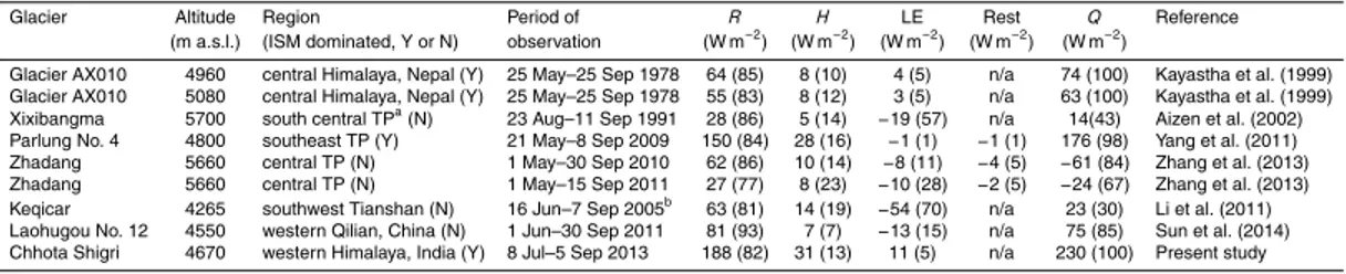
mainly in Tian Shan (Li et al., 2011), in Qilian mountains (Sun et al., 2014), in Tibetan Plateau (Yang et al., 2011; Mölg et al., 2012; Zhang et al., 2013) and in the Nepalese Hi-malaya (Kayastha et al., 1999; Lejeune et al., 2013). Unfortunately glacier SEB studies from Indian Himalaya (covering Western, some Central and Eastern parts of Himalaya) are not available. Therefore, there is an urgent need to conduct detailed SEB studies

10

in diff_{erent regions of Himalaya. In fact, SEB studies are of crucial importance because}

glaciers across the Himalayan range have diff_{erent mass balance behaviors (Gardelle}

et al., 2013), depending on their diff_{erent climatic setup. For example, glaciers in Nepal}

receive almost all their annual precipitation from the Indian summer monsoon (ISM), thus these are summer-accumulation type glaciers (Ageta and Higuchi, 1984; Wagnon

15

et al., 2013). Besides, Chhota Shigri and other glaciers in Western Himalaya receive precipitation both from the ISM in summer and from mid-latitude westerlies (MLW) in winter (Shekhar et al., 2010).

Chhota Shigri Glacier is one of the best studied glaciers in Indian Himalaya. Between 2002 and 2013, annual field measurements revealed that the glacier lost mass at a rate

20

of−0.59±0.40 m w.e. a−1(Ramanathan, 2011; Azam et al., 2014). The volume change of Chhota Shigri Glacier has also been measured between 1988 and 2010 using in-situ geodetic measurements by Vincent et al. (2013), revealing a moderate mass loss over this 2 decade-period (−3.8±2.0 m w.e. corresponding to−0.17±0.09 m w.e. a−1). Com-bining the latter result with field measurements and digital elevation models diff

erenc-25

ing from satellite images, they deduced a slightly positive or near-zero mass balance between 1988 and 1999 (+_1.0_±_{2.7 m w.e. corresponding to}+_0.09_±_{0.24 m w.e. a}−1

). Further, Azam et al. (2014) reconstructed the annual mass balances of Chhota Shi-gri Glacier between 1969 and 2012 using a degree-day approach and an accumulation

(5)

TCD

8, 2867–2922, 2014

M. F. Azam et al.

Title Page

Tables Figures

◭ ◮

Back Close

Full Screen / Esc

Discussion

P

a

per

|

Discus

sion

P

a

per

|

Discussion

P

a

per

|

Discussion

P

a

per

|

model fed by long-term meteorological data recorded at Bhuntar meteorological station (∼50 km south of the glacier, 1092 m a.s.l.) and discussed the mass balance pattern at decadal level. They also compared the decadal mass balances with meteorological variables and suggested that winter precipitation and summer temperature are almost equally important drivers controlling the mass balance pattern of this glacier. A period

5

of steady state between 1986 and 2000 and an accelerated mass wastage after 2000 were also defined.

Present studies on the climate sensitivity of Western/Indian Himalayan glaciers ei-ther come from empirical analysis at decadal level (Azam et al., 2014) or based on ba-sic comparison between meteorological variables and glacier mass balance (Koul and

10

Ganjoo, 2010), emphasizing the lack of physical understanding of the glacier–climate relationship in this region. Therefore, a detailed analysis of the SEB yet remains under-way for Western/Indian Himalayan glaciers. Use of Automatic weather station (AWS) provides the noble opportunity to obtain long and continuous records of meteorological data and to study the seasonal and inter-annual variations in SEB at point locations

15

(e.g., Oerlemans, 2000; Reijmer and Oerlemans, 2002; Mölg and Hardy, 2004). The present study is focused on the SEB analysis of Chhota Shigri Glacier, using in-situ AWS measurements. It involves two main objectives: (1) the glacier’s microclimate is analyzed, (2) an analysis of the SEB components is given and the change character-istic of each component is analyzed to give insights into the processes controlling the

20

mass balance at point scale as well as glacier scale.

2 Data and climatic settings

2.1 Study site and AWSs description

Chhota Shigri Glacier (32.28◦N, 77.58◦E) is a valley-type, non-surging glacier located in the Chandra-Bhaga river basin of Lahaul and Spiti valley, Pir Panjal range, Western

25

(6)

TCD

8, 2867–2922, 2014

M. F. Azam et al.

Title Page

Tables Figures

◭ ◮

Back Close

Full Screen / Esc

Discussion

P

a

per

|

Discus

sion

P

a

per

|

Discussion

P

a

per

|

Discussion

P

a

per

|

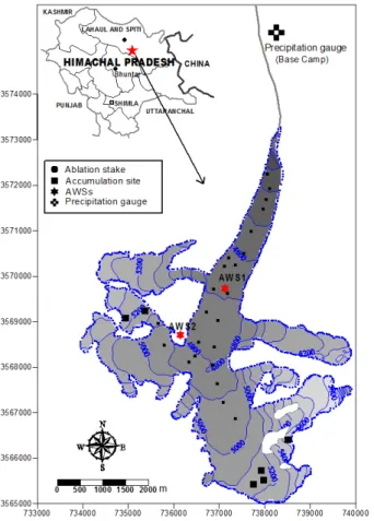
Chandra River, one of the tributaries of Indus river system. Chhota Shigri Glacier extends from 6263 to 4050 m a.s.l. with a total length of 9 km and area of 15.7 km2 (Wagnon et al., 2007). The main orientation is north in its ablation area but its tribu-taries and accumulation area have a variety of orientations (Fig. 1). The lower ablation area (<4500 m a.s.l.) is covered by debris representing approximately 3.4 % of the

to-5

tal surface area (Vincent et al., 2013). The debris layer is highly heterogeneous, from some millimeter silts to big boulders exceeding sometimes several meters. Its snout is well defined, lying in a narrow valley and giving birth to a single pro-glacial stream. The equilibrium line altitude (ELA) for a zero net balance is close to 4900 m a.s.l. (Wagnon et al., 2007). This glacier is located in the monsoon–arid transition zone and

influ-10

enced by two diff_{erent atmospheric circulation systems: the ISM during summer (July–}

September) and the Northern Hemisphere MLW during winter (January–April) (e.g., Bookhagen and Burbank, 2010).

Two meteorological stations (AWS1 and AWS2) have been operated on Chhota Shi-gri Glacier (Fig. 1). AWS1 was operated between 12 August 2012 and 4 October 2013,

15

in the middle of ablation zone (4670 m a.s.l.) on an almost horizontal and homogeneous surface while AWS2 is located off_{-glacier on a western lateral moraine (4863 m a.s.l.)}

and functioning continuously since 18 August 2009. At AWS1 and AWS2, meteoro-logical variables are recorded as half-hourly means with a 30 s time step, except for wind direction (half-hourly instantaneous values), and stored in a Campbell CR1000

20

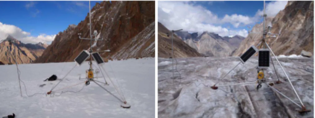
data logger. AWS1 is equipped with a tripod standing freely on the glacier with wooden plates at its legs and sinks with the melting surface. AWS2 provides pluri-annual me-teorological data (from 2009 to 2013) allowing characterization of the seasons as well as analysis of the local climatic conditions on Chhota Shigri Glacier. Both AWS1 and AWS2 were checked and maintained every month during the summers (accessibility

25

in winter was not possible). At the glacier base camp (3850 m a.s.l.), an all-weather precipitation gauge with a hanging weighing transducer (Geonor T-200B) has been op-erating continuously since 7 July 2012 (Fig. 1). Geonor sensor is suitable for both solid

(7)

TCD

8, 2867–2922, 2014

M. F. Azam et al.

Title Page

Tables Figures

◭ ◮

Back Close

Full Screen / Esc

Discussion

P

a

per

|

Discus

sion

P

a

per

|

Discussion

P

a

per

|

Discussion

P

a

per

|

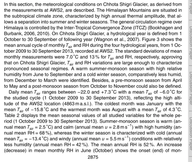
and liquid precipitation measurements. Table 1 gives the list of meteorological variables used in this study, with their specifications.

2.2 Meteorological data

Only AWS1 data were used for SEB calculations. During winter, the lower sensors (Tair,

RH,u) were buried under heavy snowfalls on 18 January 2013, and AWS1 stopped

op-5

erating completely on 11 February 2013 till 7 July 2013 when the glacier was again ac-cessible and AWS1 could be repaired. To ensure good data quality, the period between 4 and 11 February 2013 was eliminated as this period was supposed to be influenced by near surface snow. Thus, complete data set of 263 days in two separate periods (13 August 2012 to 3 February 2013 and 8 July to 3 October 2013) are available for

10

analysis, except SR50A, for which data are also missing from 8 September to 9 Oc-tober 2012. The records from AWS2 have very few data gaps (0.003 %, 0.29 %, and 0.07 % data gaps over the 4-year period forTair,uand WD, respectively). These gaps

were filled by linear interpolation using the neighboring data. Only one long gap exists for LWI data between 18 August 2009 and 22 May 2010.

15

In snow- and ice-melt models, cloud cover is investigated by computing “cloud fac-tors”, defined as the ratio of measured and modeled clear-sky solar radiation (Greuell et al., 1997; Klok and Oerlemans, 2002; Mölg et al., 2009). In the present study cloud factor is calculated by comparing SWI with solar radiation at the top of atmosphere (STOA) according to the Eq.: cloud factor =_1.3–1.4_×_(SWI_/_{STOA) that represents}

20

a quantitative cloud cover estimate. The values 1.3 (off_{set) and 1.4 (scale factor) were}

derived from a simple linear optimization process (Favier et al., 2004). The cloud fac-tor is calculated between 11:00 to 15:00 local time (LT) to avoid the shading eff_{ect of}

steep valley walls during morning and evening time. The theoretical value of STOA is calculated for a horizontal plane following the Iqbal, (1983) and considering the solar

25

(8)

TCD

8, 2867–2922, 2014

M. F. Azam et al.

Title Page

Tables Figures

◭ ◮

Back Close

Full Screen / Esc

Discussion

P

a

per

|

Discus

sion

P

a

per

|

Discussion

P

a

per

|

Discussion

P

a

per

|

2.3 Accumulation and ablation data

The SR50A sensor records the accumulation of snow (height decrease of the sensor) or the melting of ice and melting or packing of snow (height increase) at 4670 m a.s.l. close to AWS1 (Fig. 2). This sensor does not involve an internal temperature sensor to compensate the variations in speed of sound as a function ofTair. Therefore,

tem-5

perature corrections for the speed of sound were applied to the sensor output using

Tair recorded at the higher level. Measured distance may reduce during the evening

which could be misunderstood as a snowfall event (Maussion et al., 2011). In order to minimize this eff_{ect and to reduce the noise, a 3 h moving mean is applied to smooth}

the SR50A data. On Chhota Shigri Glacier, during summer-monsoon season, sporadic

10

snowfall events and follow-up melting may occur within hours. Therefore, the sensor height variations from the 3 h smoothed SR50A data should be calculated over a time interval long enough to detect the true height changes during the snowfalls and short enough to detect a snowfall before melting begins. Given that SR50A measurements have uncertainty of±1 cm, an agreement was achieved with a 6 h time step between

15

smoothed SR50 data to get surface changes by more than 1 cm.

Point mass balance was measured from ablation stake no. VI which is located at the same elevation and around 20 m south to AWS1. Frequent measurements, with inter-vals of some days to a couple of weeks, were made at stake no. VI during summer expeditions. In summer 2012, 3 stake measurements, with intervals of 10 to 15 days,

20

have been performed from 8 August to 21 September 2012 and in summer 2013, 6 measurements, with intervals of 7 to 30 days, have been carried out from 8 July to 3 October 2013. By subtracting the snow accumulation assessed from SR50A measure-ments at AWS1 (assuming a density of 0.2 for accumulated snow), the ablation was derived corresponding to every period between two stake measurements.

25

(9)

TCD

8, 2867–2922, 2014

M. F. Azam et al.

Title Page

Tables Figures

◭ ◮

Back Close

Full Screen / Esc

Discussion

P

a

per

|

Discus

sion

P

a

per

|

Discussion

P

a

per

|

Discussion

P

a

per

|

2.4 Climatic settings

2.4.1 Characterization of seasons

In this section, the meteorological conditions on Chhota Shigri Glacier, as derived from the measurements at AWS2, are described. The Himalayan Mountains are situated in the subtropical climate zone, characterized by high annual thermal amplitude, that

al-5

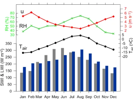
lows a separation into summer and winter seasons. The general circulation regime over Himalaya is controlled by the Inter-Tropical Convergence Zone (ITCZ) (Bookhagen and Burbank, 2006, 2010). On Chhota Shigri Glacier, a hydrological year is defined from 1 October to 30 September of following year (Wagnon et al., 2007). Figure 3 shows the mean annual cycle of monthlyTairand RH during the four hydrological years, from 1

Oc-10

tober 2009 to 30 September 2013, recorded at AWS2. The standard deviations of mean monthly measurements were 7.0◦_{C and 13 % for}_T

air and RH, respectively, approving

that on Chhota Shigri Glacier,Tair and RH variations are large enough to characterize

pronounced seasonal regimes. A warm summer-monsoon season with high relative humidity from June to September and a cold winter season, comparatively less humid,

15

from December to March were identified. Besides, a pre-monsoon season from April to May and a post-monsoon season from October to November could also be defined. Daily mean Tair ranges between −22.0 and +7.3◦C with a mean Tair of−6.0◦C for

the studied cycle (1 October 2009 to 30 September 2013), reflecting the high alti-tude of the AWS2 location (4863 m a.s.l.). The coldest month was January with the

20

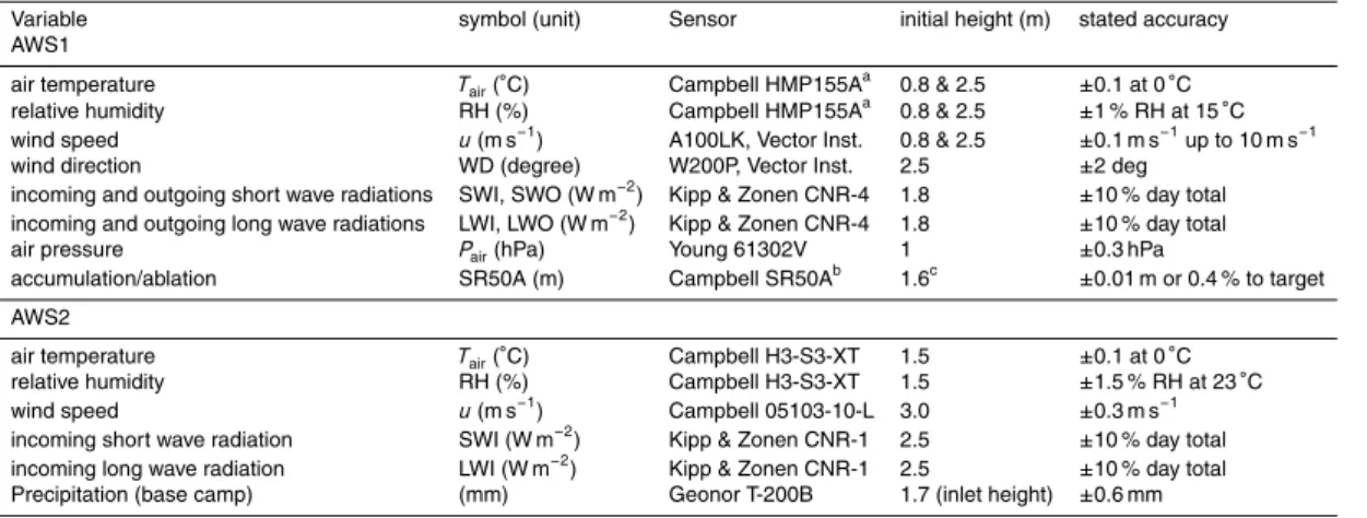
meanTair of−15.8◦C and the warmest month was August with a mean Tair of 4.3◦C.

Table 2 displays the mean seasonal values of all studied variables for the whole pe-riod (1 October 2009 to 30 September 2013). Summer-monsoon season is warm (an-nual meanT_air=_2.5◦_{C) and calm (annual mean}_u=_{2.8 m s}−1_{) with high humidity}

(an-nual mean RH=_{68 %), whereas the winter season is characterized with cold (annual}

25

meanTair=−13.4◦C) and windy (annual meanu=5.5 m s− 1

) conditions with relatively less humidity (annual mean RH=_{42 %). The mean annual RH is 52 %. An increase}

(10)

mon-TCD

8, 2867–2922, 2014

M. F. Azam et al.

Title Page

Tables Figures

◭ ◮

Back Close

Full Screen / Esc

Discussion

P

a

per

|

Discus

sion

P

a

per

|

Discussion

P

a

per

|

Discussion

P

a

per

|

soon on Chhota Shigri Glacier. The highest mean monthly RH of summer-monsoon was observed in August (74 %) while in winter maximum was observed in February (51 %) (Fig. 3), confirming that Chhota Shigri Glacier is receiving moisture alternately from ISM during summer-monsoon and MLW during winter season. Pre-monsoon and post-monsoon seasons showed intermediate conditions for air temperature, moisture

5

and wind speed (Table 2). Although during summer-monsoon season the solar angle is at its annual maximum, SWI is the highest during the pre-monsoon season with a mean value of 299 W m−2. Indeed, in summer-monsoon SWI is reduced by 33 W m−2 (summer-monsoonal mean=_{266 W m}−2_{) because of high cloud cover revealed by high}

moisture conditions (RH=_{68 % with STD}=_{1 %, Table 2). The low values of SWI,}

dur-10

ing summer-monsoon season, are compensated by high values of LWI (Fig. 3 and Ta-ble 2) mostly emitted from warm summer-monsoonal clouds. Post-monsoon and winter seasons are rather similar, receiving low and almost same SWI (176 and 161 W m−2, respectively) and LWI (187 and 192 W m−2

, respectively). The low SWI and LWI values over these seasons are mainly related to the decreasing solar angle (for SWI), and low

15

values ofTair, RH and cloudiness (for LWI), respectively.

2.4.2 Influence of ISM and MLW

The whole Himalayan range is characterized by, from west to east, the decreasing influence of the MLW and the increasing influence of the ISM (Bookhagen and Burbank, 2010), leading to distinct precipitation regimes on glaciers depending on their location.

20

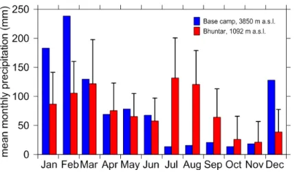
Figure 4 shows the monthly precipitations for a complete hydrological year be-tween 1 October 2012 and 30 September 2013 at Chhota Shigri Glacier base camp (3850 m a.s.l.) (Fig. 1). Surprisingly, the months with minimum precipitation were July to November (mean value of 16 mm) and those with maximum precipitation were Jan-uary and FebrJan-uary (183 and 238 mm, respectively). For the ease of understanding,

25

Wulf et al. (2010) divided the distribution of precipitation over the same region in two periods i.e. from May to October with precipitation predominantly coming from ISM and from November to April with precipitation coming from MLW. ISM contributed only 21 %

(11)

TCD

8, 2867–2922, 2014

M. F. Azam et al.

Title Page

Tables Figures

◭ ◮

Back Close

Full Screen / Esc

Discussion

P

a

per

|

Discus

sion

P

a

per

|

Discussion

P

a

per

|

Discussion

P

a

per

|

while MLW added 79 % precipitation to the annual precipitation (976 mm) at Chhota Shigri base camp for 2012/2013 hydrological year. In Fig. 5, a comparison of 2012/2013 monthly precipitation at base camp is also done with long-term (1969–2013) mean monthly precipitations at Bhuntar meteorological station, Beas basin (Fig. 1). Although this station is only about 50 km from Chhota Shigri Glacier, the precipitation regime is

5

noticeably diff_{erent because ISM and MLW equally contribute to the average annual}

precipitation (916 mm yr−1). The diff_{erent precipitation regimes in this region can be}

explained by the location of the orographic barrier which ranges between 4000 and 6600 m in elevation (Wulf et al., 2010). ISM, coming from Bay of Bengal in the south-east, is forced by the orographic barrier to ascend that enhances the condensation

10

and cloud formation (Bookhagen et al., 2005) thus, provides high precipitations in the windward side of the orographic barrier at Bhuntar meteorological station (51 % of the annual precipitation) and low precipitations in its leeward side at Chhota Shigri Glacier (21 % of annual precipitation). In contrast to the ISM, MLW moisture derived from the Mediterranean, Black, and Caspian seas is transported at higher tropospheric levels

15

(Weiers, 1995). Therefore, the winter westerlies predominantly undergo orographic capture at higher elevations in the orogenic interior providing high precipitations at Chhota Shigri Glacier (79 % of annual precipitation) compared to Bhuntar meteorologi-cal station in windward side (49 % of annual precipitation). Thus, Chhota Shigri Glacier seems to be a winter-accumulation type glacier receiving most of its annual

precipita-20

tion during winter season. This precipitation comparison between glacier base camp and Bhuntar meteorological station is only restricted to 2012/2013 hydrological year, when precipitation records at glacier base camp are available. Long-term precipita-tion data at glacier site are still required to better understand the relaprecipita-tionship between both precipitation regimes occurring on the southern and northern slopes of Pir Panjal

25

(12)

TCD

8, 2867–2922, 2014

M. F. Azam et al.

Title Page

Tables Figures

◭ ◮

Back Close

Full Screen / Esc

Discussion

P

a

per

|

Discus

sion

P

a

per

|

Discussion

P

a

per

|

Discussion

P

a

per

|

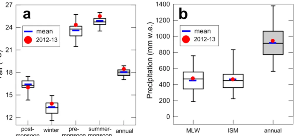
2.4.3 Representativeness of 2012/2013 hydrological year

Given that long-term meteorological data at the glacier are unavailable, the represen-tativeness of the meteorological conditions prevailing during the 2012/2013 hydrolog-ical year is assessed using Tair and precipitation data from the nearest

meteorolog-ical station at Bhuntar. Figure 5a shows the comparison of 2012/2013 Tair with the

5

long-term mean between 1969 and 2013 at seasonal as well as annual scale.Tair in

2012/2013 was systematically higher in all seasons (0.5◦_{C, 0.5}◦_{C and 0.6}◦_{C in winter,} pre-monsoon and summer-monsoon seasons, respectively) except for post-monsoon season when it was lower (0.4◦C) than mean seasonal Tair over 1969–2013 period.

At annual scale, 2012/2013 hydrological year was 0.4◦_{C warmer with}_T

air close to the

10

75th percentile of annual meanTair between 1969 and 2013 period. Figure 5b

com-pares the precipitation observed during the 2012/2013 hydrological year to the mean over the 1969–2013 period. In 2012/2013 hydrological year, both ISM (May to Octo-ber) and MLW (November to April) circulations brought almost equal amount (49 and 51 %, respectively) of precipitation at Bhuntar meteorological station. This year the ISM

15

precipitation was equal to mean ISM precipitation over 1969/2013 whereas MLW pre-cipitation was 5 % higher than mean MLW prepre-cipitation over 1969/2013 hydrological years (Fig. 5b); therefore, the annual precipitation for 2012/2013 was found slightly higher (943 mm w.e.) than mean annual precipitation (919 mm w.e.) over 1969/2013 hydrological years. In conclusion, 2012/2013 hydrological year was relatively warmer

20

with slightly higher precipitation compared to annual means over 1969–2013 period but can be considered as an average year.

(13)

TCD

8, 2867–2922, 2014

M. F. Azam et al.

Title Page

Tables Figures

◭ ◮

Back Close

Full Screen / Esc

Discussion

P

a

per

|

Discus

sion

P

a

per

|

Discussion

P

a

per

|

Discussion

P

a

per

|

3 Methodology: SEB calculations 3.1 SEB equation

The meteorological data from AWS1 were used to derive the SEB at point-scale. A unit volume of glacier is defined from the surface to a depth where no significant heat fluxes are found. On this volume, for a unit of time, and assuming a lack of horizontal energy

5

transfers, the SEB Eq. can be expressed as (e.g., Oke, 1987, p. 90):

SWI−SWO+LWI−LWO+H+LE+G+P =Q (1)

where SWI, SWO, LWI and LWO are the incident short-wave, outgoing short-wave, incoming long-wave and outgoing long-wave radiations, respectively.H and LE are the

10

sensible and latent turbulent heat fluxes, respectively.G is the conductive heat flux in the snow/ice andP is the heat supplied by precipitation.Qis the net heat flux available at glacier surface. All the fluxes (W m−2) towards the surface are taken as positive and vice-versa. The heat supplied by precipitation on glaciers is insignificant compared to the other fluxes (Oerlemans, 2001) therefore neglected here. The conductive heat

15

transfer within the snowpack or the ice is also ignored as it tends to be small when compared to radiative or turbulent fluxes (Marks and Dozier, 1992). Consequently the SEB is described by the sum of radiation fluxes and turbulent heat fluxes.

The model calculates the SEB at point scale according to Eq. (1) at a half-hourly time-step. When surface temperature (Tsurf) reaches the melting point, the

20

amount of melt M (m w.e.) is calculated from Q divided by the latent heat of fusion (3.34×105J kg−1) and the density of water (1000 kg m−3).Tsurfwas derived from LWO

using the Stefan–Boltzmann equation assuming that the emissivity of the ice/snow is unity (LWO=_σT_s4_with_σ=_5.67_×₁₀−8_{W m}−2_K−4_{) and that it cannot exceed 273.15 K.}

Here it is considered that the surface is in melting conditions whenTsurfreaches 0◦C.

(14)

TCD

8, 2867–2922, 2014

M. F. Azam et al.

Title Page

Tables Figures

◭ ◮

Back Close

Full Screen / Esc

Discussion

P

a

per

|

Discus

sion

P

a

per

|

Discussion

P

a

per

|

Discussion

P

a

per

|

3.2 Radiative fluxes

Radiation fluxes are directly measured in the field (Table 1) however several correc-tions were applied to this data before using in SEB model. Night values of SWI and SWO were set to zero. SWI is found much more sensitive to measurement uncertain-ties compared to SWO (Van den Broeke et al., 2004). At high elevation sites, such as

5

Himalaya, measured SWO can be higher than SWI (2.6 % of total data here) during the morning and evening time when the solar angle is low because of poor cosine re-sponse of the upward-looking radiation (SWI) sensor (Nicholson et al., 2013). Besides, as AWS1 was installed on the middle of the ablation area, the unstable glacier surface during ablation season conceivably give rise to a phase shift by mast tilt (Giesen et al.,

10

2009). However in these conditions, SWO sensor is slightly aff_{ected because it is}

re-ceiving isotropic radiation mostly. SWI is calculated from SWO (raw) and accumulated albedo (αacc) to elude the impact of the phase shift because of tilting during the daily

cycle of SWI and poor cosine response of the SWI sensor during the low solar angles.

αacc values were computed (Eq. 2) as the ratio of accumulated SWO (raw) and SWI

15

(raw) over a time-window of 24 h centered on the moment of observation using the method described in Van den Broeke et al. (2004). The obvious shortcoming of the accumulated albedo method is the elimination of the clear-sky daily cycle inαacc(Van

den Broeke et al., 2004).

αacc=

P

24SWO

P

24SWI

(2)

20

A correction has also been applied to long-wave radiations as the air particles between the glacier surface and CNR-4 sensor radiates and influences the LWI (underestima-tion of LWI at the surface) and LWO (overestima(underestima-tion). This generally occurs whenTair

is higher than 0◦C during summer-monsoon season (July to September). Figure 3a

25

reveals a linear relation between LWO andT_air above 0◦C. Measured LWO was often found substantially greater than 315.6 W m−2, which is the maximum possible value for

(15)

TCD

8, 2867–2922, 2014

M. F. Azam et al.

Title Page

Tables Figures

◭ ◮

Back Close

Full Screen / Esc

Discussion

P

a

per

|

Discus

sion

P

a

per

|

Discussion

P

a

per

|

Discussion

P

a

per

|

a melting glacier surface. Therefore, a correction can be done using LWO. We adopted the method described by Giesen et al. (2014) and fitted a linear function to the me-dian values of the additional LWO (greater than 315.6 W m−2) for all 0.5◦CTairintervals

above 0◦C, assuming that the correction is zero at 0◦C. This correction was added to LWI and subtracted from LWO (Fig. 6b) whenTair was higher than 0◦C. Corrections

5

have half-hourly values up to 22 W m−2 for Tair of 11◦C. Over all half-hourly periods

withTair above 0◦C, the average correction was 6.3 W m− 2

.

3.3 Turbulent fluxes

3.3.1 Turbulent flux calculations

Althoughu, Tair and RH were measured at two levels (0.8 and 2.5 m) at AWS1, the

10

bulk method is used to calculate the turbulent heat fluxes. Denby and Greuell (2000) showed that the bulk method gives reasonable results in the entire layer below the wind speed maximum even in katabatic wind conditions whereas the profile method severely underestimates these fluxes. In turn, the bulk method has already been applied in various studies where katabatic winds dominate (e.g. Klok et al., 2005; Geisen et al.,

15

2014). The major characteristic of katabatic flow is the wind speed maximum which is dependent on glacier size, slope, temperature, surface roughness and other forcing mechanisms (Denby and Greuell, 2000). At AWS1 site, uat the upper level (initially at 2.5 m) is always higher (99.6 % of all half-hourly data) than that at the lower level (initially at 0.8 m) suggesting that the wind speed maximum is almost systematically

20

above 2.5 m and justifies the choice of the bulk method.

The bulk method calculates the turbulent fluxes including stability correction. This method is usually used for practical purposes because it allows the estimation of the turbulent heat fluxes from one level of measurement (Arck and Scherer, 2002). In this approach, a constant gradient is assumed between the level of measurement and the

25

(16)

TCD

8, 2867–2922, 2014

M. F. Azam et al.

Title Page

Tables Figures

◭ ◮

Back Close

Full Screen / Esc

Discussion

P

a

per

|

Discus

sion

P

a

per

|

Discussion

P

a

per

|

Discussion

P

a

per

|

eff_{ects of buoyancy to mechanical forces (e.g., Brutsaert, 1982; Moore, 1983; Oke,}

1987):

Rib=

g(Tair−Tsurf)

(z−z0 T)

Tair

u z−z0 m

2

=g(Tair−Tsurf)(z−z0 m)

2

Tairu2(z−z0 T)

(3)

wherezis the level of measurements.Tairanduare used from the upper level that

pro-5

vides a longer period for investigation. The sensors height was extracted from SR50A records except a data gap between 8 September to 9 October 2012. Over this period sensors height were assumed to be constant and set as 2.5 m being AWS1 in free standing position. g is the acceleration of gravity (g=_{9.81 m s}−2_), _T

surf is the surface

temperature (in K).z0 mand z0 T are the surface roughness parameters (in m) for

mo-10

mentum and temperature, respectively. Assuming that local gradients of mean horizon-talu, meanTairand mean specific humidityqare equal to the finite differences between

the measurement level and the surface, it is possible to give analytical expressions for the turbulent fluxes (e.g., Oke, 1987):

H=_ρCPk

2

u(Tair−Tsurf)

ln_zz 0 m ln

z z0 T

(ΦmΦh)

−1 ₍₄₎

15

LE=_ρLSk

2

u(q−qsurf)

ln_zz 0 m ln

z z_{0 q}

(ΦmΦv)

−1

(5)

whereρ is the air density (in kg m−3) at 4670 m a.s.l. at AWS1 and calculated using ideal gas equation (ρ=Patm

R_aT, whereRabeing the specific gas constant for dry air andPair

is given by the measurements and around 565 hPa).CP is the specific heat capacity for

20

air at constant pressure (Cp=Cpd(1+0.84q) withCpd=1005 J kg− 1

K−1

(17)

TCD

8, 2867–2922, 2014

M. F. Azam et al.

Title Page

Tables Figures

◭ ◮

Back Close

Full Screen / Esc

Discussion

P

a

per

|

Discus

sion

P

a

per

|

Discussion

P

a

per

|

Discussion

P

a

per

|

heat capacity for dry air at constant pressure),k is the von Karman constant (k=_0.4)

and Ls is the latent heat of sublimation of snow or ice (Ls=2.834×10 6

J kg−1). Fur-thermore,q is the mean specific humidity (in g kg−1) of the air at the heightz andqsurf

is the mean specific humidity at surface.z0 Tandz0 qare the surface roughness

param-eters for temperature and humidity, respectively. To compute turbulent fluxes Eqs. (4)

5

and (5), it is assumed that the temperature is equal to Tsurf atz0 T and that the air is

saturated with respect to Tsurf atz0 q. The last assumption helps to calculate surface

specific humidityqsurf. The non-dimensional stability functions for momentum (Φm), for

heat (Φ_h_{) and moisture (}Φ_v_{) can be expressed in terms of Ri}_b_{(e.g., Favier et al., 2011):}

For Ri_bpositive (stable): (Φ_mΦ_h₎−1₌

(Φ_mΦ_v₎−1₌

(1−5Rib) 2

(6)

10

For Ribnegative (unstable): (ΦmΦh)−

1₌

(Φ_mΦ_v₎−1₌

(1−16Rib) 0.75

(7)

The lower and upper limits of Ri_bwere fixed at−0.4 and 0.23, respectively beyond that all turbulence is suppressed (Denby and Greuell, 2000; Favier et al., 2011).

3.3.2 Roughness parameters

15

The aerodynamic (z0 m) and scalar roughness lengths (z0 Tandz0 q) play a pivotal role

in bulk method as the turbulent fluxes are very sensitive to the choice of these surface roughness lengths (e.g., Hock and Holmgren, 1996; Wagnon et al., 1999). In several studies (e.g., Wagnon et al., 1999; Favier et al., 2004), the surface roughness lengths were all chosen equal (z0 m=z0 T=z0 q) and used as calibration parameters. In the

20

present study, the z_{0 m} was calculated assuming a logarithmic profile for wind speed between both the levels of measurements in neutral conditions (e.g., Moore, 1983):

z0 m=exp

_u

2lnz1−u1lnz2

u2−u1

(8)

whereu1 and u2 are the wind velocities measured at the lower and higher levels z1

25

(18)

TCD

8, 2867–2922, 2014

M. F. Azam et al.

Title Page

Tables Figures

◭ ◮

Back Close

Full Screen / Esc

Discussion

P

a

per

|

Discus

sion

P

a

per

|

Discussion

P

a

per

|

Discussion

P

a

per

|

time-step), it was assumed that conditions are neutral, and half-hourly values forz0 m

were calculated using the Eq. (8). Half-hourly values ofz0 m were assessed separately

for ice and snow surfaces, based on field observations (snow covered surface between 16 September 2013 and 17 January 2013 and ice-covered surface the rest of the time). Thez0 m was calculated as 0.016 m (with STD of 0.026 m) and 0.001 m (0.003 m) for

5

ice and snow surfaces, respectively. During summer-monsoon, the surface is covered with hummocks and gullies andz_{0 m}is large whereas in winter, snow covers all surface irregularities and fills up the gullies (Fig. 2) providing small values of z0 m. The ratio

between roughness lengths (zm/zq and zm/zT) depends on the Reynolds number of

the flow according to Andreas (1987) polynomials. For high Reynolds numbers

(aero-10

dynamically rough flows), the polynomials suggested by Smeets and Van den Broeke (2008) for hummocks were used. The respective mean values obtained forzT and zq

are identical and equal to 0.004 m over ice surfaces, and 0.001 m over snow surfaces. These values are similar toz0 mvalues for snow-smooth surfaces as already observed

by Bintanja and Van den Broeke (1995) and lower for icy-rough surfaces as pointed

15

out by many authors (e.g., Andreas, 1987; Hock and Holmgren, 1996; Meesters et al., 1997).

4 Results

4.1 Analysis of the meteorological conditions at AWS1

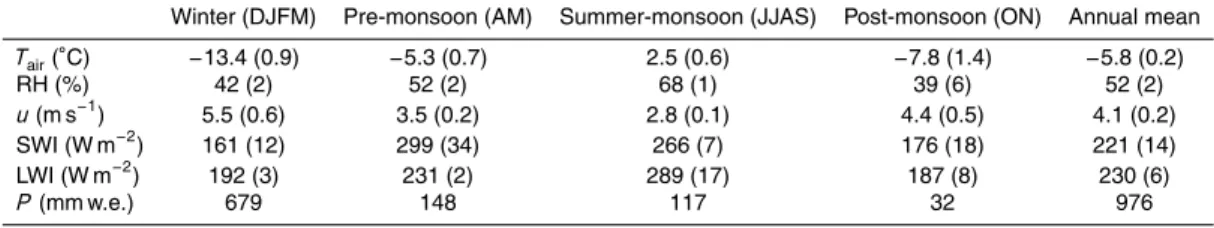
In order to understand the seasonal evolution of the physical processes controlling the

20

mass balance of the glacier, diff_{erent representative periods for various seasons were}

selected. The selected representative periods are post-monsoon (1 October 2012 to 29 November 2012), winter (1 December 2012 to 29 January 2013) and summer-monsoon (8 July 2013 to 5 September 2013). The selection of these representative periods was based on the meteorological conditions observed in Sect. 2.4 and available dataset

25

at AWS1. The same length of 60 days of each representative period was chosen for

(19)

TCD

8, 2867–2922, 2014

M. F. Azam et al.

Title Page

Tables Figures

◭ ◮

Back Close

Full Screen / Esc

Discussion

P

a

per

|

Discus

sion

P

a

per

|

Discussion

P

a

per

|

Discussion

P

a

per

|

justified comparison among diff_{erent seasons. Unfortunately data was not available for}

pre-monsoon season. Measurements (Tair, RH,uand WD) recorded at the upper level

sensors were used for the analysis, since the records from the lower level sensors have longer data gap because of early burial of sensors. A summary of the mean variables measured in diff_{erent representative periods at AWS1 is given in Table 3.}

5

Figure 7 shows the daily averages of Tair, u, RH, LWI, LWO, SWI, SWO, STOA,

cloud factor,α_acc and snow falls for all three representative periods. The meteorolog-ical variables show strong seasonality and day-to-day variability. The last panels of Fig. 7 represent the daily snowfall amounts (with a data gap between 1 and 8 Octo-ber 2012) at AWS1 site extracted from SR50A data (by applying a fresh snow density

10

of 200 kg m−3

). Post-monsoon and winter periods are cold with mean Tair andTsurf

al-ways far below freezing point (Fig. 7 and Table 3). During post-monsoon period mean

uandαaccprogressively increased (meanu=4.7 m s− 1

andαacc=0.73) and reached

their highest values in winter period (meanu=_{4.9 m s}−1

andαacc=0.79).αaccremains

almost constant in winter period showing the persistent snow cover. Snowfalls in

post-15

monsoon period were frequent but generally very light (<10 mm w.e.), whereas winter period received a substantial amount of snow (the heaviest snowfalls were observed on 16 December 2012, and 17, 18 January 2013 with 32, 44 and 80 mm w.e., respec-tively). These snowfall events are associated with high RH,αacc, cloud factor and LWI.

Obviously, an abrupt decrease of SWI (consequently low SWO) is noticed during

snow-20

fall events. Most of the time, due to very cold and dry high-elevation atmosphere, LWI remains very low during both periods, with mean values of 205 and 189 W m−2in post-monsoon and winter periods, respectively (Table 3). An analysis of Fig. 7 showed that overcast days with high cloud factor, high RH, increased LWI and decreased SWI are evident during all three representative periods.

25

(20)

TCD

8, 2867–2922, 2014

M. F. Azam et al.

Title Page

Tables Figures

◭ ◮

Back Close

Full Screen / Esc

Discussion

P

a

per

|

Discus

sion

P

a

per

|

Discussion

P

a

per

|

Discussion

P

a

per

|

low and almost constantαacc indicates that the glacier ice was exposed all the time.

During summer field expeditions the cloud formation in afternoon hours can often be observed. The surface remains almost permanently in melting conditions, as shown by constantly maximal LWO values. Although the summer-monsoon period is charac-terized by the highest values of RH (82 %) and cloud factor (0.4), little snowfall events

5

are observed from the SR50A at AWS1 site. Given thatTair was above freezing point,

the precipitation might have been occurred in the form of rain most of the time. Due to warm, humid and cloudy conditions, LWI is much higher in summer-monsoon than during the other seasons, with a mean value of 300 W m−2

(Table 3).

Post-monsoon and winter periods are characterized by high winds (meanuvalues

10

of 4.7 and 4.9 m s−1, respectively; Table 3). In summer-monsoon perioduis quite sta-ble (STD=_{0.5 m s}−1

) and gusts at minimum strength with a mean value of 3.6 m s−1

. Chhota Shigri Glacier is situated in an almost north-south oriented valley and the AWS1 site is surrounded by steep valley walls from east and west directions (Fig. 1). The scat-ter plots of uwith Tair and WD over all of the observation periods at half-hourly time

15

scale were plotted following Oerlemans (2010). Figure 8a mostly shows a linear rela-tionship betweenTairabove melting point anduat AWS1 site showing that increasingu

is associated with increasing near-surfaceTair, indicative of katabatic forcing whereas

Fig. 8b reveals a mean down-glacier wind (WD of 200–210◦) most of the time.

Although, generally, katabatic wind flow is more expected during summer season

20

than in winter (Oerlemans, 2010), Fig. 9 shows that this is not the case at AWS1 on Chhota Shigri Glacier. WD, measured at AWS1, indicates that there is a persistent down-glacier wind coming from south to southwest (200–210◦) during post-monsoon and winter periods. In winter the half-hourly meanureaches up to 10 m s−1_compared to 8 m s−1 in post-monsoon period. During both post-monsoon and winter periods the

25

glacier surface is snow covered (with high αacc, Fig. 7) and a down-glacier wind is

maintained by the negative radiation budget (Sect. 4.2) of the snow surface which gives rise to cooling to the near-surface air, generating katabatic flow (Grisogono and

(21)

TCD

8, 2867–2922, 2014

M. F. Azam et al.

Title Page

Tables Figures

◭ ◮

Back Close

Full Screen / Esc

Discussion

P

a

per

|

Discus

sion

P

a

per

|

Discussion

P

a

per

|

Discussion

P

a

per

|

Oerlemans, 2002). Occasionally, wind from south-east (160◦_{) in the direction of a large} hanging glacier was also observed.

Further, on Chhota Shigri Glacier, in summer-monsoon period the wind regime is quite remarkable. A down-glacier wind as a result of katabatic forcing, coming from south to southwest (200–210◦) is relatively weak in summer-monsoon period. Wind

5

also tends to come from south-east (160◦), in the direction of a large hanging glacier (Fig. 1). The upcoming valley wind coming from north-east (50◦_{), blowing against the} katabatic wind, is weak at the AWS1 site and appears only during summer-monsoon periods when the katabatic wind is comparatively weak. As a cumulative result of valley and katabatic winds, a wind from 110◦ _{is also observed. AWS1 is surrounded by the}

10

steep valley walls and probably the impact of synoptic wind remains feeble thus the katabatic flow is the dominated phenomenon most of the time of the year, which is typical for many glaciers (Van den Broeke, 1997).

4.2 Mean values of the SEB components

Mean SEB values for three representative periods are presented in Fig. 10 and are

re-15

ported in Table 3. The results indicate that the SWN is highly variable from a low winter mean value of 29 W m−2 _{to a very high summer-monsoon mean value of 202 W m}−2 (Table 3). Besides the seasonal changes in sun inclination, the main reason for the seasonal variability of SWN is the contrast in surface albedo in diff_{erent periods}

(Ta-ble 3). Seasonal variations in LWN are rather low, post-monsoon and winter periods

20

show minimum values of LWN (mean=₋_{57 and}₋_{49 W m}−2

, respectively) while a max-imum value was reached in summer-monsoon period (mean=₋_{13 W m}−2_{) when}

rela-tively highTsurf(mean=−0.1◦C) coincides with warm and humid conditions, associated

with intense cloud covers leading to high values of LWI. The net radiation heat fluxR

(SWN+_{LWN) was negative in post-monsoon and winter periods, giving rise to}

near-25

(22)

TCD

8, 2867–2922, 2014

M. F. Azam et al.

Title Page

Tables Figures

◭ ◮

Back Close

Full Screen / Esc

Discussion

P

a

per

|

Discus

sion

P

a

per

|

Discussion

P

a

per

|

Discussion

P

a

per

|

surface in the form ofH. The highest contribution ofH (associated with the highestu, Table 3) was in winter with a mean value of 33 W m−2(Table 3). LE was continuously negative in post-monsoon and winter periods with mean values of−25 and−20 W m−2, respectively. Therefore, surface losses mass through sublimation (corresponding to re-spective mean daily rates of 0.8 and 0.6 mm w.e. d−1). However, in summer-monsoon

5

period, a sign shift in LE from negative to positive occurred. The relatively highTairand

RH (Table 3) lead to a reversal of the specific humidity gradient and therefore a positive LE for a melting valley glacier (Oerlemans, 2000). Because of this positive LE, glacier gained mass through condensation or re-sublimation (0.3 mm w.e. d−1) of moist air at the surface (Table 3).

10

As a result of SEB, positive melt heat flux (Q), with almost the same oscillation trend as SWN (Fig. 10), occurred only in summer-monsoon period when melting conditions were prevailing all the time, leading to a mean daily melt rate of 60.9 mm w.e. d−1. During summer-monsoon period SWN accounted for 88 % of the total heat flux and was the most important heat-flux component for surface melting.R was estimated as

15

82 % of the total heat flux that was complimented with turbulent sensible and latent heat fluxes with a share of 13 % and 5 %, respectively. During post-monsoon period the glacier started cooling down (meanQ=₋_{4 W m}−2_{) and only a little melting (mean}

daily rate of 0.7 mm w.e. d−1) occurred during the noon hours only, when occasionally

Tsurf reached 0◦C, while in winter period the glacier was too cold to experience any

20

melting (meanQ=₋_{7 W m}−2_).

4.3 Model validation

The model provides a heat transfer at half-hourly time step to the glacier superficial layers that can be turned into melt when surface temperature is at 0◦C. Other possible way to lose/gain mass is from sublimation/condensation or re-sublimation. The amount

25

of sublimation/condensation or re-sublimation (m w.e.) is computed from calculated LE dividing by the latent heat of sublimation (2.834×106J kg−1) and the density of water (1000 kg m−3

(23)

TCD

8, 2867–2922, 2014

M. F. Azam et al.

Title Page

Tables Figures

◭ ◮

Back Close

Full Screen / Esc

Discussion

P

a

per

|

Discus

sion

P

a

per

|

Discussion

P

a

per

|

Discussion

P

a

per

|

the SEB model, computed ablation (melt+_{sublimation) was compared with the}

abla-tion measured at stake no. VI in the field (Sect. 2.3). The correlaabla-tion between computed ablation from the SEB Eq. and measured ablation at stake no. VI is strong (r2=_0.98,

n=_{9 periods) indicating the robustness of the model. However, the computed}

abla-tion is 1.10 times higher than the measured one (Fig. 11), but this diff_{erence (10 %}

5

overestimation) is acceptable given the overall uncertainty of 140 mm w.e. in stake ab-lation measurements (Thibert et al., 2008). The SEB model can, therefore, generate an acceptable computation of point mass balance.

4.4 Mean diurnal cycle of the meteorological variables and SEB components The mean diurnal cycles of the meteorological variables and SEB components for all

10

three representative periods are shown in Fig. 12. Mean diurnal cycles ofTsurf

(equiv-alent to LWO) andTair showed that the glacier was in freezing conditions during

post-monsoon and winter periods all the time (Fig. 12) while in summer-post-monsoonTsurfis

al-ways at melting point in agreement with consistent positiveT_air. Occasionally, for some days, half-hourly meanTair(not shown here) may drop below freezing point during night

15

in summer-monsoon and go above freezing point during noon hours in post-monsoon period. A wind speed maximum is observed in the afternoon hours during all the rep-resentative periods, which is consistent with Tair. This is a common phenomenon on

valley glaciers,uincreases in the afternoon (e.g., Van den Broeke, 1997; Greuell and Smeets, 2001) as a consequence of an increased glacier wind due to a strongerTair

20

deficit in the afternoon.

For all the representative periods,Ris negative at night (indicating long-wave radia-tive cooling of the surface) and posiradia-tive during day time. However, during the summer-monsoon period the night values ofRare slightly less negative as the radiative cooling is attenuated due to enhanced RH,Tairand cloudiness, in turn high LWI. In daytime,R

25

(24)

TCD

8, 2867–2922, 2014

M. F. Azam et al.

Title Page

Tables Figures

◭ ◮

Back Close

Full Screen / Esc

Discussion

P

a

per

|

Discus

sion

P

a

per

|

Discussion

P

a

per

|

Discussion

P

a

per

|

H and LE show similar trends in post-monsoon and winter periods. In the night, H

remains permanently high (∼50 W m−2) and starts decreasing in the morning as the surface is heated up with R (Fig. 12). This daily cycle of H is in agreement with the daily cycle of Rib, showing stable conditions almost all day long (Rib>0 except 4 h

in the middle of the afternoon in winter), with very stable conditions in the night, and

5

moderately stable during the day or even unstable in the afternoon in winter. LE is slightly negative in the night, decreases in the morning and shows the minimum values during early afternoon hours which are in agreement with increasing wind speed and stronger vertical gradients of specific humidity in the vicinity of the surface. During summer-monsoon, bothH and LE are positive (heat supplied to the surface) and follow

10

a similar trend, butH attains its peak approximately 2 h before LE.H shows a peak at ∼14:00 LT with positive Tair and wind speed maximum (Fig. 12) whereas LE remains

close to 0 W m−2until noon and increases with an afternoon wind speed maximum. The stability of the surface boundary layer is not very diff_{erent from that observed during}

the other periods, highly stable at night, but moderately stable during the day due to

15

the occurrence of warm up-valley winds blowing over a melting surface in summer-monsoon. Thus, LE is positive during summer-monsoon giving rise to condensation or re-sublimation in afternoon and early night hours.

During post-monsoon and winter periods, in the night and even during afternoon hours in winter,Q is negative, and a cold front penetrates into the superficial layers of

20

the glacier. However, Q is rather low as R is mostly compensated by H+_{LE except}

during noon hours whenQswitches to slightly positive values. Heat is then transferred during a few hours of the day to the ice/snow pack whose temperature rises but not enough to reach melting conditions (Tsurfremains below 0◦C) (Fig. 12). During

summer-monsoon period,Qfollows the diurnal cycle ofR providing energy up to 740 W m−2 to

25

the glacier surface at around 13:00 LT. This energy is consumed for melting process as the surface is in melting conditions permanently (Fig. 12). Unfortunately, the dataset does not cover the pre-monsoon season. But during this season, the heat transferred to the glacier progressively increases as net short-wave radiation enhances in agreement

(25)

TCD

8, 2867–2922, 2014

M. F. Azam et al.

Title Page

Tables Figures

◭ ◮

Back Close

Full Screen / Esc

Discussion

P

a

per

|

Discus

sion

P

a

per

|

Discussion

P

a

per

|

Discussion

P

a

per

|

with the rise of the solar angle, as well as the decreasing surface albedo. This heat is first used to warm up the surface layers of the glacier until Tsurf reaches 0◦C, then

melting starts.

5 Discussion

5.1 Control of summer-monsoon snowfalls on melting

5

Changes in the Asian monsoon climate and associated glacier responses have be-come predominant topics of climate research in High Asia Mountains (e.g., Mölg et al., 2012). Previously, based on a degree-day approach, Azam et al. (2014) suggested that winter precipitation and summer temperature are almost equally important drivers con-trolling the mass balance pattern of Chhota Shigri Glacier. Here this topic is addressed

10

by analyzing the glacier melting on Chhota Shigri Glacier with summer-monsoon pre-cipitations using more detailed SEB approach. Based on the available dataset, we se-lected the same length of summer-monsoon period (15 August to 30 September) from 2012 and 2013 years to compare the evolution of the computed cumulative melting (Fig. 13). Given that the SR50A at AWS1 site has a data gap between 8

Septem-15

ber to 9 October 2012 and that this sensor cannot record rain events, daily precipita-tions, collected at glacier base camp (3850 m a.s.l.), are used in this analysis. These precipitations can be considered as rain (snow) at AWS1 site when T_air at AWS1 is above (below) 1◦C (e.g., Wagnon et al., 2009). In summer-monsoon 2012 Chhota Shigri Glacier received one important snowfall on 17–19 September of 25 mm w.e.

20

(equivalent to 125 mm of fresh snow applying a density of 200 kg m−3). This snow-fall abruptly changed the surface conditions by varying the surface albedo from 0.19 to 0.73 (Fig. 13a). Therefore, the energy Q available at the glacier surface suddenly dropped from 125 W m−2 on 16 September to 14 W m−2 on 17 September as shown by the sharp change in the melting rate (slope of the melting curve on Fig. 13a)

as-25