DURABILITY OF THERMAL RENDERING AND
PLASTERING SYSTEMS
JOANA FERNANDES MAIA DOCTORAL THESIS PRESENTED TO
FACULTY OF ENGINEERING OF UNIVERSITY OF PORTO IN CIVIL ENGINEERING
DURABILITY
OF
THERMAL
RENDERING
AND
PLASTERING
SYSTEMS
J
OANAF
ERNANDESM
AIAMaster in Building Construction of Faculty of Engineering of University of Porto
Doctoral Thesis submitted to obtain the Doctor Degree in Civil Engineering
Supervisor: Professor Nuno Manuel Monteiro Ramos
Co-Supervisor: Doctor Maria do Rosário Veiga
Fax +351-22-508 1446 [email protected]
Edited by
FACULDADE DE ENGENHARIA DA UNIVERSIDADE DO PORTO Rua Dr. Roberto Frias
4200-465 PORTO Portugal Phone. +351-22-508 1400 Fax +351-22-508 1440 [email protected] http://www.fe.up.pt
Partial reproduction of this document is allowed provided that credit is given to the author and to Programa Doutoral em Engenharia Civil - Departamento de Engenharia Civil, Faculdade de Engenharia da Universidade do Porto, Porto, Portugal.
The opinions and information included herein solely represent the point of view of the author. The Editor cannot accept any legal liability or otherwise for errors or omissions that may exist.
To my family Para a minha família
ACKNOWLEDGEMENTS
A long-term work, such as a Doctoral Thesis, is the result of several joint efforts and not only an individual process. It requires different knowledge, which is applied during all the process in the distinct phases. The most insignificant contribute may be the key to complete the puzzle that is the Doctoral Thesis.
I wish to thank Professor Nuno Ramos, my thesis supervisor, for all the support and friendship during all these years. For believing in my capacities, in my skills and encouraging me to achieve more and more knowledge. To Doctor Maria do Rosário Veiga, my co-supervisor, for the untiring commitment. Allways available, assertive and meticulous. For all the support in the visits to LNEC, which were crucial to the development of the experimental works. Thank you, Professor Nuno and Engineer Rosário for the readiness, guidance, suggestions and affection. I am lucky for having you both in my professional path.
My special thanks to Saint-Gobain Weber, especially to Luís Silva and Hélder Gonçalves, to Sival – Gessos Especiais, especially to Ângela Sousa, to Secil Argamassas, especially to Dina Frade and to Fradical, especially to Engineer Cartaxo, for the execution of all the specimens and technical support. To FCT-Fundação para a Ciência e a Tecnologia, the funding of the Doctoral Grant PD/BD/52659/2014, through the Doctoral Programme EcoCoRe. I also would like to thank to EcoCoRe Professors and Collegues the wise advices and the good moments during the Summer Schools.
This work was financially supported by UID/ECI/04708/2019- CONSTRUCT - Instituto de I&D em Estruturas e Construções funded by national funds through the FCT/MCTES (PIDDAC).
This work was financially supported by Project PTDC/ECI-CON/28766/2017 and POCI-01-0145-FEDER-028766 funded by FEDER funds through COMPETE2020 - Programa Operacional Competitividade e Internacionalização (POCI) and by national funds (PIDDAC) through FCT/MCTES. To all the Professors and Colleagues of LFC-CONSTRUCT for being always there in this long journey, especially to Sara, for the support with climatic data, and to my long-standing friend Pedro. To Professor Luísa Sousa from Mechanical Engineer Department of FEUP, the support in the thermo-mechanical simulation with ABAQUS software.
To all the laboratory technicians and colleagues of the Building Coatings and Thermal Insulation Unit of LNEC, especially to Acácio Monteiro and Dora Santos for the support in the experimental campaign, to Luís Matias in the obtention of thermograms, to Catarina Farinha and Cláudio Cruz in the use of the optical microscope, to Ana Marques for showing me the best material ever to bonding the Karsten tubes, to Sofia Malanho and Bento Sabala for the scientific and technical advices.
To Music and to God! I have no doubt that it was crucial to have balance, peace and joy!
To the most important part of my life: Friends and Family! To my special friends Claudia, Sara, Filipe, Ana and Hugo, for being like family! To Alexandra and Bruno, for receiving me at their home in the several working visits to LNEC. To my godson Bernardo, to my godfather Rogério, to my aunts and uncles, to my cousins, especially to the kindest girl, my cousin Vera. To the joy of my life, my nieces Margarida and Maria, to my dear brother Nuno, to my love Bruno, to the most wonderful and exceptional people in the world, my mother Fernanda and my father Horácio. Obrigada por me ensinarem os verdadeiros valores da vida!
ABSTRACT
The increase of thermal demands in buildings and the changes in the European thermal regulations implied the decrease of the thermal transmission of building envelopes. As such, researchers and manufacturers started searching for new solutions, such as thermal renders and plasters. However, a gap in the durability assessment of thermal rendering and plastering systems was observed, since the existing standardization for the durability assessment of hardened mortars does not allow a consistent evaluation, considering thermal mortars, especially in multilayer systems.
Therefore, the main goal of this Doctoral Thesis consisted of the development and implementation of durability assessment methodologies applicable to thermal rendering and plastering systems. The methodology used to achieve this main objective was based on the analysis of the characteristics and specificities of thermal rendering and plastering systems, the related existing standards and methodologies for the durability assessment and, throughout numerical simulation and laboratory tests, presenting specific methodologies for the durability assessment of this type of systems.
The determination of the physical, hygrothermal and mechanical properties allowed deepening the knowledge of thermal renders/plasters and systems, contributing to develop more reliable simulations. The determination of the most relevant properties allowed observing important findings, such as the high contribution of the capillary network in increasing the moisture content and therefore the increase of the thermal conductivity. The thermal renders/plaster presented low water vapour resistance comparing to EPS (expanded polystyrene), allowing higher water vapour exchanges, which contributes to greater compatibility with ancient materials, than low vapour permeability materials. Regarding the adhesive strength, these systems presented low adhesive strength, but in the order of magnitude of ETICS (External Thermal Insulation Composite Systems).
The numerical simulation allowed evaluating the most significant degradation mechanisms and the related failure modes of thermal rendering and plastering systems. The hygrothermal simulation highlighted the great impact of the finishing coatings in the water content of the inner layers. The thermo-mechanical simulation showed a reduction of the thermal induced stresses in thermal systems with low differences of rigidity between the thermal and finishing renders. Thermal rendering systems present lower condensation potential than the studied ETICS, for the same insulation thickness. A behavioural dependence of thermal rendering systems on climate conditions and material properties was observed.
The lack of durability assessment procedures directly applicable to thermal rendering and plastering systems motivated the development of a new durability assessment methodology, filling the existing gap. The methodology takes into account the intrinsic properties of the materials that constitute the system, the type of application (exterior or interior), the climatic conditions and consequent degradation mechanisms to which the system will be subjected. The knowledge of these parameters allows defining the accelerated ageing cycles that reproduce the real degradation mechanisms. The combination of the analysis of existing procedures with the hygrothermal simulation allowed the development of accelerated ageing hygrothermal cycles, applied to thermal rendering systems, taking into account the European climatic context, throughout a theoretical algorithm.
KEYWORDS: Thermal rendering and plastering systems, Durability, Accelerated ageing, Material properties, Experimental tests, Hygrothermal performance, Thermo-mechanical performance, Numerical simulation.
RESUMO
O aumento das exigências térmicas nos edifícios e as alterações às regulamentações térmicas europeias tiveram implicação na redução da transmissão térmica da envolvente dos edifícios. Como tal, investigadores e fabricantes procuraram desenvolver novas soluções, como rebocos térmicos. No entanto, observou-se uma lacuna no que diz respeito à avaliação da durabilidade de sistemas de reboco térmico, visto que os procedimentos normalizados existentes para a avaliação da durabilidade de argamassas endurecidas não permite uma avaliação consistente de argamassas térmicas, especialmente se inseridas em sistemas multicamada.
Portanto, o principal objetivo desta Tese de Doutoramento consistiu no desenvolvimento e implementação de metodologias de avaliação da durabilidade aplicáveis a sistemas de reboco térmico. A metodologia utilizada para atingir este objetivo principal baseou-se na análise das características e especificidades dos sistemas de reboco térmico, nas normas e metodologias existentes para a avaliação da durabilidade e no desenvolvimento de metodologias específicas para a durabilidade deste tipo de sistemas, através de simulação numérica e ensaios laboratoriais.
A determinação das propriedades físicas, higrotérmicas e mecânicas permitiu aprofundar o conhecimento sobre rebocos térmicos e sistemas, contribuindo o mesmo para o desenvolvimento de simulações numéricas mais confiáveis. A determinação das propriedades mais relevantes permitiu observar uma grande contribuição da rede capilar no aumento do teor de humidade e, consequentemente, no aumento da condutibilidade térmica. Os rebocos térmicos apresentaram baixa resistência ao vapor de água em comparação com EPS, permitindo maiores trocas de vapor de água e contribuindo para uma maior compatibilidade com materiais antigos, do que materiais com baixa permeabilidade ao vapor. Quanto à aderência, os rebocos térmicos apresentaram baixa resistência, porém da ordem de grandeza de ETICS correntes.
A simulação numérica permitiu avaliar os mecanismos de degradação mais significativos e os modos de rotura relacionados com sistemas de reboco térmico. A simulação higrotérmica evidenciou o grande impacto das camadas de acabamento no teor de água das camadas internas. A simulação termomecânica permitiu observar uma redução das tensões induzidas por ação térmica em sistemas com menores diferenças de rigidez entre as camadas de reboco térmico e de acabamento. Os sistemas de reboco térmico apresentaram menor potencial de condensação do que o ETICS analisado, para a mesma espessura de isolamento. Observou-se uma relação de dependência dos sistemas de reboco térmico com as diferentes condições climáticas e as propriedades dos materiais.
A inexistência de procedimentos de avaliação da durabilidade diretamente aplicáveis a sistemas de reboco térmico motivou o desenvolvimento de uma nova metodologia de avaliação da durabilidade, colmatando a lacuna existente. A metodologia tem em consideração as propriedades intrínsecas dos materiais que constituem o sistema, o tipo de aplicação (exterior ou interior), as condições climáticas e consequentes mecanismos de degradação a que estará sujeito. O conhecimento destes parâmetros permite definir os ciclos de envelhecimento acelerado que reproduzam os mecanismos de degradação reais. A combinação da análise de procedimentos existentes com a simulação higrotérmica permitiu o desenvolvimento de ciclos higrotérmicos de envelhecimento acelerado, aplicados a sistemas de reboco térmico, tendo em conta o contexto climático europeu, através de um algoritmo teórico.
PALAVRAS-CHAVE:Sistemas de reboco térmico, Durabilidade, Envelhecimento acelerado, Propriedades dos materiais, Ensaios laboratoriais, Desempenho higrotérmico, Desempenho termo-mecânico, Simulação numérica.
CONTENTS 1. INTRODUCTION ... 1 1.1. Motivation ... 1 1.2. Objectives ... 4 1.3. Methodology ... 5 1.4. Thesis outline ... 6
2. STATE OF THE ART... 9
2.1. Framework ... 9
2.2. Thermal wall systems ... 9
2.2.1. Introduction ... 9
2.2.2. Binders and lightweight aggregates ... 13
2.2.3. Thermal renders and plasters ... 15
2.2.3.1. Cement and lime based mortars with thermal characteristics ... 15
2.2.3.2. Gypsum-based plasters with thermal characteristics ... 23
2.2.4. Other thermal wall systems ... 27
2.3. Sustainability, eco-construction and durability ... 30
2.3.1. Sustainability and eco-construction ... 30
2.3.2. Durability and service life prediction ... 34
2.4. Degradation agents and mechanisms in thermal mortars... 37
2.5. Durability assessment ... 41
2.5.1. Principles and standards ... 41
2.5.2. Accelerated ageing ... 41
2.5.3. Standard procedures of durability assessment ... 43
2.5.4. Non-standardized procedures of durability assessment of non-traditional mortars ... 45
2.6. Synthesis of the chapter ... 48
3. EXPERIMENTAL CHARACTERISATION OF THERMAL RENDERING AND PLASTERING SYSTEMS ... 57
3.1. Materials and experimental methodology ... 57
3.1.1. Introduction ... 57
3.1.2. Selected thermal rendering and plastering systems ... 57
3.1.3. Experimental methods to determine the physical and hygrothermal properties ... 60
3.1.3.1. Introduction ... 60
3.1.3.2. Density, porosity and pore size distribution ... 61
3.1.3.4. Emissivity ... 64
3.1.3.5. Capillary water absorption ... 65
3.1.3.6. Moisture storage function ... 67
3.1.3.7. Water vapour permeability... 68
3.1.4. Experimental methods to determine the mechanical properties ... 69
3.1.4.1. Dynamic elastic modulus ... 69
3.1.4.2. Flexural and compressive strength ... 70
3.1.4.3. Adhesive strength ... 71
3.1.4.4. Impact resistance ... 73
3.2. Experimental results ... 73
3.2.1. Physical and hygrothermal properties ... 73
3.2.1.1. Density, porosity and pore size distribution ... 73
3.2.1.2. Thermal conductivity and emissivity ... 77
3.2.1.3. Capillary absorption ... 80
3.2.1.4. Moisture storage function ... 81
3.2.1.5. Water vapour permeability... 82
3.2.2. Mechanical properties ... 83
3.2.2.1. Dynamic elastic modulus ... 83
3.2.2.2. Flexural and compressive strength ... 84
3.2.2.3. Adhesive strength ... 85
3.2.2.4. Impact resistance ... 92
3.2.3. Summary ... 96
4. NUMERICAL SIMULATION OF DEGRADATION MECHANISMS ... 103
4.1. Framework ... 103
4.2. Hygrothermal impact on façades with thermal rendering and plastering systems application 104 4.2.1. Modelling Principles ... 104
4.2.2. Simulation model and input data ... 108
4.2.3. Hygrothermal performance indexes ... 115
4.2.3.1. Temperature ... 115
4.2.3.2. Thermal transmission coefficient ... 119
4.2.3.3. Water content ... 122
4.2.3.4. Condensation risk ... 126
4.2.4. Summary ... 129
4.3. Thermo-mechanical impact on façades with thermal rendering and plastering systems application ... 130
4.3.1. Modelling principles ... 130
4.3.2. Simulation model and input data ... 133
4.3.3. Influence of the temperature variation in the thermal render/plaster layer surfaces ... 139
4.3.4. Influence of the thermal shock in the exterior surface ... 145
4.3.5. Influence of the type of substrate ... 148
4.3.6. Summary ... 152
5. DURABILITY ASSESSMENT OF THERMAL RENDERING AND PLASTERING SYSTEMS .... 155
5.1. Framework ... 155
5.2. Evaluation of existing methodologies of durability assessment ... 162
5.2.1. Materials and experimental methodology... 162
5.2.2. Experimental results – adapted methodology from EN 1015-21 ... 167
5.2.2.1. Liquid water permeability ... 167
5.2.2.2. Adhesive strength ... 169
5.2.2.3. Impact resistance ... 180
5.2.2.4. Visual observation and porous structure ... 186
5.2.3. Experimental results – adapted methodology from ETAG 004 ... 190
5.2.3.1. Liquid water permeability ... 190
5.2.3.2. Adhesive strength ... 191
5.2.3.3. Impact resistance ... 196
5.2.3.4. Visual observation and porous structure ... 200
5.2.4. Summary ... 203
5.3. Development of a new accelerated ageing hygrothermal cycle ... 204
5.3.1. Framework ... 204
5.3.2. Development of the heat-cold cycle ... 205
5.3.3. Development of the heat-rain cycle ... 206
5.4. Implementation of the developed accelerated ageing hygrothermal cycle ... 207
5.4.1. Specimen configuration ... 207
5.4.2. Experimental results ... 212
5.4.2.1. Visual observation ... 212
5.4.2.2. Liquid water permeability ... 216
5.4.2.3. Porous structure ... 216
5.4.2.4. Surface temperature ... 218
5.4.2.5. Ultrasonic pulse velocity ... 223
5.4.2.6. Dynamic modulus ... 225
5.4.2.8. Adhesive strength ... 227
5.4.2.9. Water content ... 232
5.4.2.10. Impact resistance ... 233
5.5. Analysis of the implemented durability assessment methodologies ... 238
5.5.1. Experimental methodologies for the durability assessment ... 238
5.5.2. Developed hygrothermal ageing cycle – Experimental results vs. numerical simulation 242 5.6. Durability assessment methodologies ... 247
5.6.1. Methodologies applicable to thermal rendering and plastering systems ... 247
5.6.2. Theoretical methodology for the definition of heat-cold cycles in Europe ... 253
6. CONCLUSIONS ... 261
6.1. Final conclusions ... 261
6.2. Future developments ... 267
REFERENCES ... 269
ANNEXES ... 285
ANNEX 1 – WUFI Pro database materials ... 285
ANNEX 2 – Simulation scenarios ... 287
ANNEX 3 – Temperature indexes ... 291
INDEX OF FIGURES
Fig. 1 – CO2 emissions from the manufacturing and the construction industries (% total fuel combustion)
(The World Bank 2014). ... 1
Fig. 2 – Evolution of the construction sector in Portugal, in the last decades – New construction vs. Rehabilitation (INE 2015). ... 2
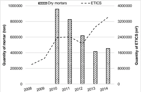
Fig. 3 – Evolution of the use of industrial dry mortars and ETICS, in Portugal (APFAC 2015b). ... 3
Fig. 4 – Evolution of the use of renders, in Portugal (APFAC 2015b)... 4
Fig. 5 – Thesis methodology. ... 6
Fig. 6 – Interconnection of the different areas presented in the state of the art. ... 9
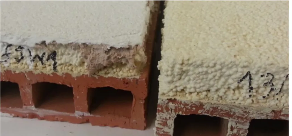
Fig. 7 – a) Example of a thermal render system: 1. Finishing coat; 2. Base coat/finishing render; 3. Glass fibre mesh; 4. Thermal render; 5. Substrate; b) Application of thermal render by mechanical spraying. ... 11
Fig. 8 – Example of an ETICS: a) 1: Substrate; 2: Adhesive mortar; 3: Thermal insulation; 4: Base coat; 5: Glass fibre mesh; 6: Finishing coating; b) Fixation through mechanical fasteners. ... 12
Fig. 9 – Evolution of ETICS in Portugal (APFAC 2015b). ... 13
Fig. 10 – Three pillars of sustainability (Perman et al. 2003). ... 31
Fig. 11 – Evolution of the main concerns in the construction sector (Bourdeau 1998)... 32
Fig. 12 – Porous net distribution according to Setzer (CEB 1992). ... 40
Fig. 13 – Porous net: porosity vs. permeability (Concrete Society 1987). ... 40
Fig. 14 – Photographs of: a) TR1; b) C1 and c) S1. ... 58
Fig. 15 – Photographs of: a) TR2; b) C2 and c) S2. ... 58
Fig. 16 – Photographs of: a) TR3; b) C3 and c) S3. ... 59
Fig. 17 – Photographs of: a) TR4; b) C4 and c) S4. ... 59
Fig. 18 – a) Drying chamber WTC Binder; b) Placement of the specimens in the drying chamber. .... 61
Fig. 19 – a) Desiccator and vacuum device; b) Hydrostatic weighing. ... 62
Fig. 20 – a) Optical microscope Olympus SZH10; b) Zoom of the specimen area. ... 62
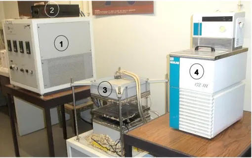
Fig. 21 – Holometrix GHP-300: 1) Temperature control; 2) Data acquisition; 3) Test specimens container; 4) Cooling device. ... 63
Fig. 22 – Test specimens container. ... 63
Fig. 23 – CT-Metre equipment: hot-wire method. ... 64
Fig. 24 – Detail of the used “anneau” probe connected to the CT-Metre. ... 64
Fig. 25 – Emissometer Model AE1 Emittance Measurements, using a Port Adapter Model AE-ADP. 65 Fig. 26 – Specimen placement for capillary absorption determination according to EN ISO 15148. ... 65
Fig. 27 – a) Climatic chamber Vötsch VC 4034; b) Placement of the specimens for the determination of the moisture storage functions. ... 67
Fig. 28 – a) Placement of the specimens in the climatic chamber; b) Sealing of the sides of the specimen
with paraffin wax, in a metallic cup. ... 68
Fig. 29 – a) Equipment for the determination of the dynamic elastic modulus; b) Longitudinal measurement... 69
Fig. 30 – Testing equipment for flexural and compressive strength determination. ... 70
Fig. 31 – a) Flexural strength test; b) Compressive strength test. ... 71
Fig. 32 – a) Testing machine Proceq DY-216; b) Testing machine attached to the glued pull-head. .. 71
Fig. 33 – Samples used to determine the adhesive strength of a thermal render system (left) and a thermal render itself (right). ... 72
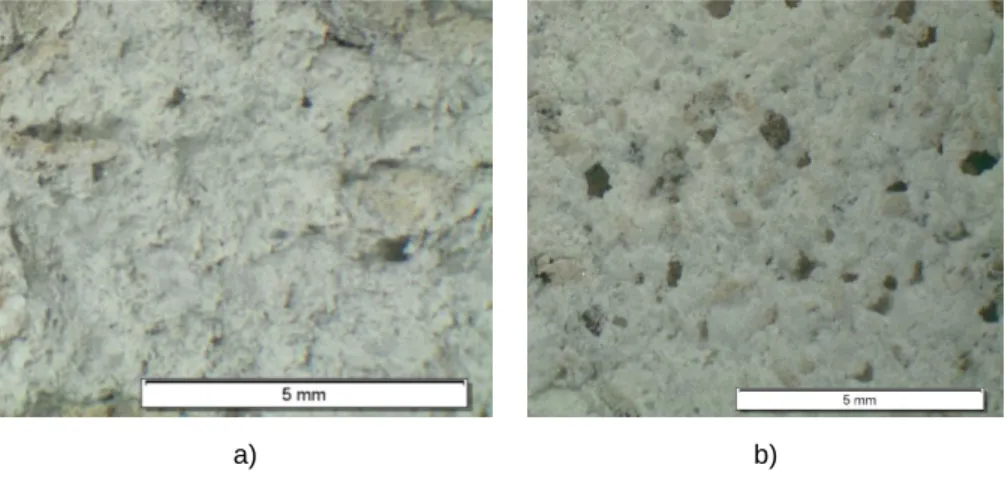
Fig. 34 – Optical microscope images: a) TR1; b) C1; c) Finishing coating of S1. ... 75
Fig. 35 – Optical microscope images: a) TR2; b) C2; c) Finishing coating of S2. ... 75
Fig. 36 – Optical microscope images: a) TR3; b) C3. ... 75
Fig. 37 – Optical microscope images: a) TR4; b) C4. ... 76
Fig. 38 – Pore size distributions of TR1 and TR2: a) Cumulative pore volume and b) Incremental pore volume. ... 76
Fig. 39 – Correlation between Guarded Hot Plate and Hot-Wire methods to determine thermal conductivity, in the dry state. ... 78
Fig. 40 – Thermal conductivity as a function of bulk density. ... 78
Fig. 41 – Thermal conductivity as a function of moisture content. ... 79
Fig. 42 – Capillary absorption as a function of the square root of time. ... 80
Fig. 43 – Capillary absorption obtained according to ETAG 004 for: a) S1, S2 and S3 and b) Detailed results of S1 and S2. ... 81
Fig. 44 – Specimens after the compressive strength test: a) TR1 and b) TR2. ... 84
Fig. 45 – Dry bulk density as a function of the open porosity and capillary water absorption coefficient, considering the analysed thermal mortars. ... 97
Fig. 46 – Liquid transport coefficient for suction as a function of the moisture content, in TR1 and TR2. ... 98
Fig. 47 – Liquid transport coefficient for suction as a function of the moisture content, in TR3. ... 98
Fig. 48 – Dynamic modulus, compressive and flexural strength as a function of the bulk density, in the thermal mortars (TR1, TR2 and TR3). ... 99
Fig. 49 – Dynamic modulus, compressive and flexural strength as a function of the bulk density, in the finishing mortars (C1, C2 and C3). ... 99
Fig. 50 – Dent diameter obtained by the hard body impact as a function of the bulk density, in the thermal mortars (TR1, TR2 and TR3). ... 100
Fig. 51 – Typical moisture storage function of building materials, as a function of the relative humidity (IBP 2016). ... 107
Fig. 52 – Solar radiation and driving rain sum, depending on the orientation: Porto climate (IBP 2016). ... 109
Fig. 53 – Solar radiation and driving rain sum, depending on the orientation: Nancy climate (IBP 2016).
... 110
Fig. 54 – Solar radiation and driving rain sum, depending on the orientation: Oslo climate (IBP 2016). ... 110
Fig. 55 – Cumulative frequency of exterior air temperature in Porto, Nancy and Oslo. ... 111
Fig. 56 – Cumulative frequency of exterior air vapour pressure in Porto, Nancy and Oslo. ... 111
Fig. 57 – Model configuration: application of thermal rendering system (exterior surface). ... 112
Fig. 58 – Model configuration: application of thermal plastering system (interior surface). ... 112
Fig. 59 – Schematic representation of the temperature indexes. ... 116
Fig. 60 – Maximum exterior surface temperature (Tse), considering south and west orientation and solar absorption of: a) 0.27 and b) 0.80. ... 117
Fig. 61 – 99th percentile of the temperature difference between the thermal render layer surfaces (∆TTR), considering south and west orientation and solar absorption of: a) 0.27 and b) 0.80. ... 118
Fig. 62 – Maximum temperature difference between the insulation layer surfaces (∆TTR), considering south and west orientation and solar absorption of: a) 0.27 and b) 0.80. ... 118
Fig. 63 – Thermal effusivity as a function of thermal conductivity and density, for the studied thermal renders/plaster and EPS. ... 119
Fig. 64 – Monthly ratio between average and reference U-value in Porto, considering the 4 orientations (N, S, E, W) and solar absorption of: a) 0.27 and b) 0.80. ... 121
Fig. 65 – Monthly ratio between average and reference U-value in Nancy, considering the 4 orientations (N, S, E, W) and solar absorption of: a) 0.27 and b) 0.80. ... 122
Fig. 66 – Monthly ratio between average and reference U-value in Oslo, considering the 4 orientations (N, S, E, W) and solar absorption of: a) 0.27 and b) 0.80. ... 122
Fig. 67 – Monthly water content in the insulation layer in Porto, considering the 4 orientations (N, S, E, W) and solar absorption of: a) 0.27 and b) 0.80... 123
Fig. 68 – Monthly water content in the insulation layer in Nancy, considering the 4 orientations (N, S, E, W) and solar absorption of (a) 0.27 and (b) 0.80. ... 123
Fig. 69 – Monthly water content in the insulation layer in Oslo, considering the 4 orientations (N, S, E, W) and solar absorption of: a) 0.27 and b) 0.80... 124
Fig. 70 – Box-plot of the water content in the thermal render layer of S1 and S2 with solar absorption of 0.27 and 0.80, in the north façade... 124
Fig. 71 – Box-plot of the water content in the thermal render layer of S1 and S2 with solar absorption of 0.27 and 0.80, in the south façade. ... 124
Fig. 72 – Box-plot of the water content in the thermal render layer of S1 and S2 with solar absorption of 0.27 and 0.80, in the east façade. ... 125
Fig. 73 – Box-plot of the water content in the thermal render layer of S1 and S2 with solar absorption of 0.27 and 0.80, in the west façade. ... 125
Fig. 74 – Ratio between the average water content and the free water saturation in the TR, considering the 4 orientations (N, S, E, W) and solar absorption of: a) 0.27 and b) 0.80. ... 125
Fig. 75 – Ratio between the maximum water content and the free water saturation in the TR, considering the 4 orientations (N, S, E, W) and solar absorption of: a) 0.27 and b) 0.80. ... 126 Fig. 76 – Accumulated positive condensation potential considering the 4 orientations (N, S, E, W) and solar absorption of: a) 0.27 and b) 0.80. ... 127 Fig. 77 – Schematic representation of the 3D simulation model with: a) Exterior insulation application (S1, S2 and ETICS); b) Interior insulation application (S3). ... 134 Fig. 78 – Temperature profile in S1, considering a solar absorption coefficient of 0.27, in: a) Porto; b) Nancy; c) Oslo. ... 136 Fig. 79 – Temperature profile in S1, considering a solar absorption coefficient of 0.80, in: a) Porto; b) Nancy. ... 137 Fig. 80 – Temperature profile in S2, considering a solar absorption coefficient of 0.27, in: a) Porto; b) Nancy; c) Oslo. ... 137 Fig. 81 – Temperature profile in S2, considering a solar absorption coefficient of 0.80, in: a) Porto; b) Nancy. ... 137 Fig. 82 – Temperature profile in ETICS, considering a solar absorption coefficient of 0.27, in: a) Porto; b) Nancy; c) Oslo. ... 138 Fig. 83 – Temperature profile in ETICS, considering a solar absorption coefficient of 0.80, in: a) Porto; b) Nancy. ... 138 Fig. 84 – Temperature profile in S3, considering a solar absorption coefficient of 0.27, in: a) Porto; b) Nancy; c) Oslo. ... 138 Fig. 85 – Non-deformed shape of half wall. ... 139 Fig. 86 – Typical deformed shape in Porto, using S1, S2 and ETICS, considering a solar absorption coefficient of: a) 0.27; b) 0.80. ... 140 Fig. 87 – Typical deformed shape in Nancy and Oslo, using S1, S2 and ETICS, considering a solar absorption coefficient of: a) 0.27; b) 0.80. ... 140 Fig. 88 – Typical deformed using S3 in: a) Porto; b) Nancy and Oslo. ... 141 Fig. 89 – Maximum strains obtained in Porto with S1, for a solar absorption coefficient of: a) 0.27; b) 0.80. ... 142 Fig. 90 – Typical minimum principal strains in the thermal rendering system, in Nancy, for a solar absorption coefficient of 0.27, considering exterior application. ... 143 Fig. 91 – Compressive stresses as a function of: a) Porosity and density; and; b) Dynamic elastic modulus and thermal expansion coefficient, of TR1, TR2 and EPS. ... 143 Fig. 92 – Typical deformed shape after: a) Heating; b) Abrupt decrease. ... 146 Fig. 93 – Strains distribution in the façade surface of ETICS after: a) Heating; b) Abrupt decrease. . 146 Fig. 94 – Tensile stresses as a function of the ratio between the dynamic elastic modulus of the finishing render (EC) and the thermal render/EPS (ETR). ... 147
Fig. 95 – Distribution of the tensile stresses after heating (70 ºC) in: (a) Thermal render TR1; (b) EPS. ... 147 Fig. 96 – Strains profile after heating (70 ºC) in: a) S1; b) S2 and c) ETICS. ... 148
Fig. 97 – Strains profile after the abrupt decrease of temperature (15 ºC) in: a) S1; b) S2 and c) ETICS.
... 148
Fig. 98 – Typical deformed shape after heating, using: a) Aerated concrete; b) Brick masonry; c) OSB. ... 149
Fig. 99 – Typical deformed shape after the abrupt decrease, using: a) Aerated concrete; b) Brick masonry; c) OSB. ... 149
Fig. 100 – Tensile stresses in the TR as a function of the elastic modulus of the substrate. ... 150
Fig. 101 – Stresses distribution in the inner surface of the thermal render after heating, using: a) Aerated concrete; b) Brick masonry; c) OSB. ... 151
Fig. 102 – Strains profile after heating, using: a) Aerated concrete; b) Brick masonry; c) OSB. ... 151
Fig. 103 – Strains profile after the abrupt decrease, using: a) Aerated concrete; b) Brick masonry; c) OSB. ... 152
Fig. 104 – Framework of existing durability assessment methodologies, applicable to renders and thermal multilayer systems. ... 156
Fig. 105 – Methodological process for the durability assessment of thermal rendering/plastering systems. ... 156
Fig. 106 – Durability experimental methodology. ... 157
Fig. 107 – Köppen-Geiger climate classification (Benmansour et al. 2014). ... 158
Fig. 108 – Durability assessment methodology. ... 160
Fig. 109 – Test specimens for durability tests according to the adapted methodology from EN 1015-21: a) TR1; b) TR2... 162
Fig. 110 – Constitution of the thermal rendering system S1 for the durability tests. ... 162
Fig. 111 – Constitution of the thermal rendering system S2 for the durability tests. ... 163
Fig. 112 – Constitution of the thermal plastering system S3 for the durability tests. ... 163
Fig. 113 – Finishing coatings of thermal render system S1: a) Organic (S1-O); b) Mineral (S1-M). .. 164
Fig. 114 – Solamagic Infra-Red (IR) lamp device. ... 164
Fig. 115 – Deep freeze cabinet SMEG EL5=SCO 50. ... 165
Fig. 116 – Large waterproof container: a) Side view; b) Interior view. ... 165
Fig. 117 – Inconclusive thermal render water permeability test. ... 165
Fig. 118 – Water permeability test using the: a) Adapted methodology from EN 1015-21; b) Karsten tubes method. ... 166
Fig. 119 – Water permeability test results using the cone method: a) S1 and S2, after heating-freezing and humidification-freezing ageing cycles; b) S3, after heating-freezing ageing cycles... 167
Fig. 120 – Water distribution in S3, after 1h: a) Before ageing; b) After heating-freezing ageing cycles. ... 168
Fig. 121 – Gypsum coating (C3) degradation: a) Detachment and loss of material; b) Cracking and dissolution. ... 168
Fig. 122 – Water permeability test results using the Karsten tubes method: a) S1 and S2, after heating-freezing and humidification-heating-freezing ageing cycles; b) S3, after heating-heating-freezing ageing cycles. ... 169
Fig. 123 – Adhesive strength of thermal renders TR1 and TR2 before (BA) and after (AA) heating-freezing and humidification-heating-freezing ageing cycles... 172 Fig. 124 – Adhesive strength of thermal rendering and plastering systems before (BA) and after (AA) heating-freezing and humidification-freezing ageing cycles. ... 179 Fig. 125 – Average adhesive strength of thermal renders/plaster and systems before (BA) and after (AA) heating-freezing and humidification-freezing ageing cycles. ... 179 Fig. 126 – Average dent diameter before (BA) and after (AA) heating-freezing and humidification-freezing ageing cycles for an impact of: a) 2J; b) 10J. ... 180 Fig. 127 – Visual observation of S3, after heating-freezing ageing cycles. ... 186 Fig. 128 – Optical microscope images of TR1: a) Before ageing; b) after heating-freezing and humidification-freezing ageing cycles. ... 187 Fig. 129 – Optical microscope images of S1-O after heating-freezing and humidification-freezing ageing cycles. ... 187 Fig. 130 – Optical microscope images of S1-M after heating-freezing and humidification-freezing ageing cycles: a) TR1; b) Mineral coating. ... 188 Fig. 131 – Optical microscope images of TR1 (2.5x), after heating-freezing and humidification-freezing ageing cycles: a) Organic coating; b) Mineral coating. ... 188 Fig. 132 – Optical microscope images of TR2: a) Before ageing; b) after heating-freezing and humidification-freezing ageing cycles. ... 189 Fig. 133 – Optical microscope images of S2 after heating-freezing and humidification-freezing ageing cycles: a) TR2; b) Finishing coating. ... 189 Fig. 134 – Optical microscope images of S3 after heating-freezing ageing cycles: a) TR3; b) C3. ... 190 Fig. 135 – Water permeability test results of S1 and S2, after freeze-thaw ageing cycles, using the: a) Cone method; b) Karsten tubes method. ... 191 Fig. 136 – Fracture patterns obtained in S1-O, after freeze-thaw ageing cycles: a) Specimens overview; b) Detailed view. ... 192 Fig. 137 – Example of the adhesive fractures obtained in S1-M, after freeze-thaw ageing cycles. ... 192 Fig. 138 – Adhesive strength of thermal rendering systems S1-O, S1-M and S2 before (BA) and after (AA) after freeze-thaw ageing cycles. ... 196 Fig. 139 – Average dent diameter before (BA) and after (AA) after freeze-thaw ageing cycles for an impact of: a) 2J; b) 10J. ... 197 Fig. 140 – Visual observation of S1-O: a) before; b) after ageing according to ETAG 004 procedure. ... 200 Fig. 141 – Visual observation of S1-M: a) before; b) after freeze-thaw ageing cycles. ... 200 Fig. 142 – a) Damage of the coating; b) Cracks on the sealant, after freeze-thaw ageing cycles. .... 201 Fig. 143 – Deterioration of the thermal render layer, after freeze-thaw ageing cycles. ... 201 Fig. 144 – Optical microscope images of S1-O after freeze-thaw ageing cycles: a) TR1; b) C1; c) Organic coating. ... 202 Fig. 145 – Optical microscope images (2.5x) of S1-M after freeze-thaw ageing cycles: a) TR1; b) Mineral coating. ... 202
Fig. 146 – Optical microscope images of S2 after freeze-thaw ageing cycles: a) TR2 (0.7x); b) TR2 (2.5x); c) Coating (7x). ... 203 Fig. 147 – Adopted methodology for the definition of the heat-cold cycle. ... 205 Fig. 148 – Heat-cold cycle definition: a) Comparison of the obtained temperatures in the thermal render layer, in the cycle and real climate; b) Defined heat-cold cycle. ... 206 Fig. 149 – Defined heat-rain cycle. ... 207 Fig. 150 – Wall preparation – Day 1: a) Substrate preparation; b) Application of the 1st layer of TR1.
... 208 Fig. 151 – Wall preparation – Day 1: a); Regularization of TR1; b) 1st layer of glass fibre mesh application;
c) Mechanical fixations application. ... 208 Fig. 152 – Wall preparation – Day 2: a) Application of the 2nd layer of TR1; b) After TR1 application.
... 209 Fig. 153 – Wall preparation – Day 8: a) After 3 days curing; b) Profile after 3 days curing. ... 209 Fig. 154 – Wall preparation – Day 8: a); Reinforcement of the corners; b) Reinforcement of the opening corners; c) Finishing render (C1) application. ... 210 Fig. 155 – Wall preparation – Day 8: Application of the: a) 2nd glass fibre mesh; b) Reinforcement mesh
(central zone)... 210 Fig. 156 – Wall preparation – Day 11: Application of S1-O: a) Primer; b) Organic coating. ... 211 Fig. 157 – Wall preparation – Day 11: Application of S1-M: a) Mineral coating; b) Detailed view. ... 211 Fig. 158 – Wall configuration after curing: a) Face view; b) Profile view. ... 212 Fig. 159 – Overview of the wall surface, after heat-cold cycles. ... 213 Fig. 160 – Cracks in the corners of the opening, using organic coating: a) Bottom left corner; b) Upper left corner. ... 213 Fig. 161 – Cracks in the corners of the opening, using mineral coating: a) Bottom left corner; b) Upper left corner. ... 213 Fig. 162 – Cracks in the corners of the opening, using mineral coating: a) Bottom left corner; b) Bottom right corner. ... 214 Fig. 163 – Overview of the wall surface, after heat-rain cycles. ... 214 Fig. 164 – Overview of the coatings surface, after heat-rain cycles: a) Organic; b) Mineral. ... 215 Fig. 165 – Overview of the wall surface, after one week of the end of the heat-rain cycles: a) Whole panel; b) Development of microcracks in the mineral coating side. ... 215 Fig. 166 – Water permeability test results, before and after the hygrothermal cycles (HC+HR), using the Karsten tubes method. ... 216 Fig. 167 – Optical microscope images of TR1: a) Before ageing; b) After hygrothermal cycles, with organic coating; c) After hygrothermal cycles, with the mineral coating. ... 217 Fig. 168 – Optical microscope images after hygrothermal cycles of: a) TR1, only with finishing render; b) Detailed view of the interconnection between TR1 (yellow) and C1 (pink). ... 217 Fig. 169 – Optical microscope images of C1: a) Before ageing; b) After hygrothermal cycles. ... 218
Fig. 170 – Optical microscope images of the organic coating: a) Before ageing; b) After hygrothermal cycles. ... 218 Fig. 171 – Optical microscope images of the mineral coating: a) Before ageing; b) After hygrothermal cycles. ... 218 Fig. 172 – Distribution and numbering of the thermocouples. ... 219 Fig. 173 – Surface temperature cumulative frequencies in the current zone during: a) Heat-cold cycles and b) Heat-rain cycles. ... 220 Fig. 174 – Surface temperature cumulative frequencies in the current zone, reinforced zone and openings during: a) Heat-cold cycles and b) Heat-rain cycles. ... 221 Fig. 175 – Thermograms after heat-cold cycles: a) General overview; b) Expanded view... 222 Fig. 176 – Thermograms of the opening zone, after heat-cold cycles, with: a) Organic coating; b) Mineral coating. ... 222 Fig. 177 – Measurement of the ultrasonic pulse velocity: a) Tester; b) Transducers and scale. ... 223 Fig. 178 – Ultrasonic pulse velocity test: distance vs. time, obtained in the organic coating in: a) Current zone; b) Reinforced zone (double mesh). ... 223 Fig. 179 – Ultrasonic pulse velocity test: distance vs. time, obtained in the mineral coating in: a) Current zone; b) Reinforced zone (double mesh). ... 224 Fig. 180 – Ultrasonic pulse velocity test: distance vs. time, obtained in the finishing render in: a) Current zone; b) Reinforced zone (double mesh). ... 224 Fig. 181 – Ultrasonic pulse velocity before and after hygrothermal ageing cycles. ... 225 Fig. 182 – Dynamic modulus of TR1, with organic and mineral coatings, before and after hygrothermal ageing cycles. ... 226 Fig. 183 – Flexural and compressive strength in TR1, with organic and mineral coatings, before and after hygrothermal ageing cycles. ... 227 Fig. 184 – Adhesive strength test apparatus: a) Core drilling machine; b) Testing machine. ... 228 Fig. 185 – Pre-cut into the substrate: a) Cutting zone; b) Resulting specimen. ... 228 Fig. 186 –Adhesive strength of thermal rendering systems before (BA) and after ageing: a) Single values; b) Average values. ... 231 Fig. 187 – Aspect of the thermal render after the hygrothermal ageing with: a) Organic coating and b) Mineral coating. ... 232 Fig. 188 – Martinet-Baronie apparatus, with impact energy of: a) 3 Joules; b) 10 Joules. ... 233 Fig. 189 – Average dent diameter after hygrothermal ageing cycles... 234 Fig. 190 – Water permeability, determined with Karsten tubes method, after ageing procedures with: a) Organic coating and b) Mineral coating. ... 239 Fig. 191 – Adhesive strength of thermal rendering systems, after the ageing procedures. ... 240 Fig. 192 – Average dent diameter with hard body impact, after ageing procedures considering: a) 2/3J impact energy; b) 10J impact energy. ... 240 Fig. 193 – Exterior surface temperature obtained during the heat-cold cycle: simulation vs. implementation. ... 242
Fig. 194 – Schematic representation of the wall specimen. ... 243 Fig. 195 – Maximum principal stresses, after heating period. ... 243 Fig. 196 – Minimum principal stresses, after cooling period. ... 244 Fig. 197 – Deformed shape and displacements after simulation of the: a) Heating period; b) Cooling period. ... 244 Fig. 198 – Minimum principal stresses after: a) Heating period; b) Cooling rain period. ... 245 Fig. 199 – a) Maximum principal stresses after the heating period; b) Minimum principal stresses after the cooling period. ... 246 Fig. 200 – Vectorial representation of the: a) Maximum principal stresses after the heating period; b) Minimum principal stresses after the cooling period. ... 246 Fig. 201 – Vectorial representation of the stresses after the heating period in the perpendicular planes to the TR interfaces: a) xx axis (S11); b) zz axis (S33). ... 247 Fig. 202 – Methodology of application of thermal rendering and plastering systems. ... 247 Fig. 203 – Preliminary durability assessment methodology applicable to thermal plastering systems. ... 249 Fig. 204 – Durability assessment methodology applicable to thermal rendering systems for exterior application. ... 250 Fig. 205 – European climates distribution used in the definition of the theoretical linear regressions for the heat-cold cycles determination – Group A. ... 253 Fig. 206 – Methodology for the definition of the theoretical algorithm for the heat and cold cycles temperatures determination. ... 254 Fig. 207 – Theoretical linear regressions for the heat-cold cycles determination. ... 256 Fig. 208 – European climates distribution used in the validation of the theoretical linear regressions for the heat-cold cycles determination – Group B. ... 257 Fig. 209 – Liquid transport coefficient for suction of: a) Aerated concrete block and b) Exterior render (IBP 2016). ... 286 Fig. 210 – a) Liquid transport coefficient for suction of gypsum plaster and b) Thermal conductivity, moisture-dependent: EPS (IBP 2016). ... 286 Fig. 211 – Box-plot of the water content in the insulation layer of ETICS and S3 with solar absorption of 0.27 and 0.80, in the north façade... 293 Fig. 212 – Box-plot of the water content in the insulation layer of ETICS and S3 with solar absorption of 0.27 and 0.80, in the south façade. ... 293 Fig. 213 – Box-plot of the water content in the insulation layer of ETICS and S3 with solar absorption of 0.27 and 0.80, in the east façade. ... 293 Fig. 214 – Box-plot of the water content in the insulation layer of ETICS and S3 with solar absorption of 0.27 and 0.80, in the west façade. ... 294 Fig. 215 – Box-plot of the ratio between the water content and the free water saturation in the TR of S1 and S2 with solar absorption of 0.27 and 0.80, in the north façade. ... 294 Fig. 216 – Box-plot of the ratio between the water content and the free water saturation in the TR of S1 and S2 with solar absorption of 0.27 and 0.80, in the south façade. ... 294
Fig. 217 – Box-plot of the ratio between the water content and the free water saturation in the TR of S1 and S2 with solar absorption of 0.27 and 0.80, in the east façade. ... 295 Fig. 218 – Box-plot of the ratio between the water content and the free water saturation in the TR of S1 and S2 with solar absorption of 0.27 and 0.80, in the west façade. ... 295
INDEX OF TABLES
Table 1 – Requirements applied to thermal insulating mortars according to EN 998-1 (CEN 2010). .. 12 Table 2 – Properties of cement, bims granules and EPS mortars studied by Dylewski and Adamczyk (2014). ... 16 Table 3 – Properties of thermal mortars studied by Brites, Frade and Santos (2014) ... 16 Table 4 – Properties of industrial and traditional thermal mortars measured by Vale et al. (2014). ... 17 Table 5 – Properties of a thermal lime based-mortar with cork addition studied by Sousa, Frade and Santos (2014). ... 18 Table 6 – Density and thermal conductivity of white cement mortar with different cork additions measured by Cherki et al. (2014b). ... 18 Table 7 – Obtained results from the first phase of the experimental campaign, for hardened mortars (Braga, de Brito and Veiga 2012). ... 20 Table 8 – Results from the second phase of the experimental campaign, for hardened mortars (Oliveira, de Brito and Veiga 2013). ... 21 Table 9 – Measured properties at 90 days (Velosa and Veiga 2008). ... 22 Table 10 –Experimental results of a lime plaster without metakaolin and the optimum lime-metakaolin mixture Vejmelková et al. (2012). ... 23 Table 11 – Density and thermal conductivity of gypsum-cork plasters developed by Hernández-Olivares et al. (1999). ... 24 Table 12 – Density and thermal conductivity of gypsum-cork plasters, with different cork granules size, developed by Cherki et al. (2014a). ... 24 Table 13 – Thermal properties obtained for a gypsum-vermiculite plaster by Melo et al. (2012). ... 25 Table 14 – Thermal conductivity of gypsum-based plasters vs. % of mineral addition determined by Martias et al. (2013). ... 25 Table 15 – Thermal conductivity and porosity vs. % of mineral addition measured by Abidi et al. (2015). ... 26 Table 16 – Density, thermal conductivity and porosity vs. volume ratio (White PFW/Plaster) determined by Gutiérrez-González et al. (2012b). ... 26 Table 17 – Density, thermal conductivity and porosity vs. volume ratio (PAW/Plaster) determined by Gutiérrez-González et al. (2012a). ... 27 Table 18 – Categories of degradation agents in terms of nature and class (ISO 2011). ... 37 Table 19 – Degradation mechanisms of mortars, according to Addleson (1992) and Aguiar, Cabrita and Appleton (2002). ... 38 Table 20 – Summary of the studies on mortar degradation mechanisms nature. ... 39 Table 21 – Accelerated ageing series, according to EN 1015-21 (CEN 2002a). ... 43 Table 22 – Accelerated ageing series of ETICS performed on the rig, according to ETAG 004 (EOTA 2013). ... 44
Table 23 – Accelerated ageing series of ETICS performed on small scale samples, according to ETAG 004 (EOTA 2013). ... 44 Table 24 – Other relevant standard durability assessment methodologies, based on freeze-thaw ageing, applied on mortars. ... 44 Table 25 – Non-standardized accelerated ageing hygrothermal cycles. ... 45 Table 26 – Accelerated ageing cycles with relative humidity variation. ... 46 Table 27 – Freeze-thaw cycles presented in several research studies. ... 47 Table 28 – Accelerated ageing daily cycle defined by Norvaišiene et al. (2013). ... 48 Table 29 – Summary of the main properties obtained in the research studies, for cement and lime based thermal mortars. ... 51 Table 30 – Summary of the main properties obtained in the research studies, for cement and lime-based mortars. ... 52 Table 31 – Summary of the main properties obtained in the research studies, for gypsum-based mortars. ... 54 Table 32 – Summary of the degradation mechanisms, actions, agents, failures and conditions of failure occurrence on mortars. ... 55 Table 33 – Constituent materials of the studied thermal rendering and plastering systems. ... 58 Table 34 – Materials/specimens and corresponding experimental tests and standards. ... 60 Table 35 – Water vapour permeability test conditions. ... 68 Table 36 – Loading rate related to the expected adhesive strength. ... 72 Table 37 – Density and open porosity measured by hydrostatic weighing method. ... 74 Table 38 – Density and open porosity measured by MIP/HP method. ... 74 Table 39 – Thermal conductivity and emissivity at dry state. ... 77 Table 40 – Capillary absorption coefficient results... 80 Table 41 – Moisture storage function results. ... 82 Table 42 – Water vapour permeability for dry and wet cup tests. ... 82 Table 43 – Dynamic elastic modulus results. ... 83 Table 44 – Flexural and compressive strength results. ... 84 Table 45 – Adhesive strength: average results. ... 85 Table 46 – Adhesive strength and fracture patterns obtained in TR1. ... 86 Table 47 – Adhesive strength and fracture patterns obtained in TR2. ... 87 Table 48 – Adhesive strength and fracture patterns obtained in TR3. ... 88 Table 49 – Adhesive strength and fracture patterns obtained in S1. ... 89 Table 50 – Adhesive strength and fracture patterns obtained in S2. ... 90 Table 51 – Adhesive strength and fracture patterns obtained in S3. ... 91 Table 52 – Dent diameter of the hard body impact: average results. ... 92 Table 53 – Visual observation of the dent obtained by hard body impact in TR1 and S1. ... 93
Table 54 – Visual observation of the dent obtained by hard body impact in TR2 and S2. ... 94 Table 55 – Visual observation of the dent obtained by hard body impact in TR3 and S3. ... 95 Table 56 – Thermal rendering systems classification according to hard body impact, based on the ETAG 004 requirements. ... 96 Table 57 – Summary of the mechanical properties of the studied materials (average values). ... 101 Table 58 – Summary of the hygrothermal properties of the studied materials (average values). ... 102 Table 59 – Relation between experimentally measured properties and their application as input data in simulation programs. ... 104 Table 60 – Input data in WUFI Pro: Measured material properties of system S1. ... 113 Table 61 – Input data in WUFI Pro: Measured material properties of system S2. ... 113 Table 62 – Input data in WUFI Pro: Measured material properties of system S3. ... 114 Table 63 – Input data in WUFI Pro: Material properties of simulated system ETICS. ... 114 Table 64 – Temperature indicators obtained in system S1, for the south and west orientations. ... 116 Table 65 – Temperature indicators obtained in system S2, for the south and west orientations. ... 116 Table 66 – Temperature indicators obtained in ETICS, for the south and west orientations... 117 Table 67 – Temperature indicators obtained in S3, for the south and west orientations. ... 117 Table 68 – Thermal transmission indexes obtained in system S1. ... 120 Table 69 – Thermal transmission indexes obtained in system S2. ... 120 Table 70 – Thermal transmission indexes obtained in system ETICS... 121 Table 71 – Thermal transmission indexes obtained in system S3. ... 121 Table 72 – Condensation potential indexes. ... 128 Table 73 – Material properties used in the thermo-mechanical simulation. ... 135 Table 74 – Boundary constraints of the 1st analysis: surface temperature. ... 136
Table 75 – Principal stresses obtained by temperature variation in the thermal rendering and plastering system interfaces in a central node of the façade. ... 142 Table 76 – Displacements obtained by temperature variation in the insulation layer in a central node of the façade. ... 144 Table 77 – Tensile and compressive stresses obtained by thermal shock in a central node of the façade. ... 145 Table 78 – Displacements obtained by thermal shock in a central node of the façade. ... 145 Table 79 – Tensile and compressive stresses obtained in the thermal render layer surfaces, with different substrates. ... 150 Table 80 – Displacements obtained in the thermal render layer surfaces, with different substrates. . 150 Table 81 – European climatic sub-division according to the air temperature (EOTA 1999) ... 158 Table 82 – European climatic sub-division according to the air temperature and UV radiation (EOTA 1999) ... 159
Table 83 – Classification of European climates according to the air temperature, regarding the % of occurrence in winter ... 161 Table 84 – Classification of European climates according to the air temperature, regarding the % of occurrence in summer. ... 161 Table 85 – Classification of European climates according to the average temperature of the warmest month of the year. ... 161 Table 86 – Constitution of the thermal rendering and plastering systems for the durability tests. ... 163 Table 87 – Volume of water penetration before (BA) and after (AA) heating-freezing and humidification-freezing ageing cycles. ... 167 Table 88 – Adhesive strength and fracture patterns obtained in TR1, after heating-freezing and humidification-freezing ageing cycles. ... 170 Table 89 – Adhesive strength and fracture patterns obtained in TR2, after heating-freezing and humidification-freezing ageing cycles. ... 171 Table 90 – Adhesive strength and fracture patterns obtained in S1-O, before ageing. ... 173 Table 91 – Adhesive strength and fracture patterns obtained in S1-O, after heating-freezing and humidification-freezing ageing cycles. ... 174 Table 92 – Adhesive strength and fracture patterns obtained in S1-M, before ageing. ... 175 Table 93 – Adhesive strength and fracture patterns obtained in S1-M, after heating-freezing and humidification-freezing ageing cycles. ... 176 Table 94 – Adhesive strength and fracture patterns obtained in S2, after heating-freezing and humidification-freezing ageing cycles. ... 177 Table 95 – Adhesive strength and fracture patterns obtained in S3, after heating-freezing ageing cycles. ... 178 Table 96 – Average dent diameter of the hard body impact, after heating-freezing and humidification-freezing ageing cycles. ... 180 Table 97 – Visual observation of the dent obtained by hard body impact in S1-O, before and after heating-freezing and humidification-freezing ageing cycles. ... 182 Table 98 – Visual observation of the dent obtained by hard body impact in S1-M, before and after heating-freezing and humidification-freezing ageing cycles. ... 183 Table 99 – Visual observation of the dent obtained by hard body impact in S2, before and after heating-freezing and humidification-heating-freezing ageing cycles... 184 Table 100 – Visual observation of the dent obtained by hard body impact in S3, before and after heating-freezing and humidification-heating-freezing ageing cycles... 185 Table 101 – Thermal rendering systems classification according to hard body impact, based on the ETAG 004 requirements. ... 186 Table 102 – Volume of water penetration before (BA) and after (AA) freeze-thaw. ... 190 Table 103 – Adhesive strength and fracture patterns obtained in S1-O, after freeze-thaw ageing cycles. ... 193 Table 104 – Adhesive strength and fracture patterns obtained in S1-M, after freeze-thaw ageing cycles. ... 194
Table 105 – Adhesive strength and fracture patterns obtained in S2, after freeze-thaw ageing cycles. ... 195 Table 106 – Average dent diameter of the hard body impact, after freeze-thaw ageing cycles. ... 196 Table 107 – Visual observation of the dent obtained by hard body impact in S1, after freeze-thaw ageing cycles. ... 198 Table 108 – Visual observation of the dent obtained by hard body impact in S2, before and after freeze-thaw ageing cycles. ... 199 Table 109 – Thermal rendering systems classification according to hard body impact, based on the ETAG 004 requirements. ... 200 Table 110 – Wall specimen preparation – tasks and curing times. ... 207 Table 111 – Surface temperatures during heat-cold ageing cycles. ... 220 Table 112 – Flexural and compressive strength results. ... 226 Table 113 – Adhesive strength and fracture patterns obtained in S1-O, after the hygrothermal ageing cycles. ... 229 Table 114 – Adhesive strength and fracture patterns obtained in S1-M, after the hygrothermal ageing cycles. ... 230 Table 115 – Adhesive strength and fracture patterns obtained in C1, after the hygrothermal ageing cycles. ... 231 Table 116 – Water content variation after one week of the end of the hygrothermal ageing cycles. . 232 Table 117 – Average dent diameter of the hard body impact, after hygrothermal ageing cycles. ... 233 Table 118 – Visual observation of the dent obtained by hard body impact in S1-O, after hygrothermal ageing cycles. ... 235 Table 119 – Visual observation of the dent obtained by hard body impact in S1-M, after hygrothermal ageing cycles. ... 236 Table 120 – Visual observation of the dent obtained by hard body impact in C1, after hygrothermal ageing cycles. ... 237 Table 121 – Thermal rendering systems classification according to hard body impact, based on the ETAG 004 requirements. ... 238 Table 122 – Temperature indicators used in the definition of the theoretical algorithm for the heat-cold cycles – Group A. ... 255 Table 123 – Temperature indicators used in the validation of the theoretical algorithm for the heat-cold cycles – Group B. ... 258 Table 124 – Physical and hygrothermal properties of aerated concrete, exterior render and gypsum plaster used in the hygrothermal simulations (IBP 2016). ... 285 Table 125 – Simulation scenarios for exterior application – Porto climate. ... 287 Table 126 – Simulation scenarios for exterior application – Nancy climate. ... 288 Table 127 – Simulation scenarios for exterior application – Oslo climate... 289 Table 128 – Simulation scenarios for thermal plastering system S3 – interior application. ... 290 Table 129 – Temperature indicators obtained in system S1, for the north and east orientations. ... 291
Table 130 – Temperature indicators obtained in system S2, for the north and east orientations. ... 291 Table 131 – Temperature indicators obtained in ETICS, for the north and east orientations. ... 291 Table 132 – Temperature indicators obtained in S3, for the north and east orientations. ... 292
NOMENCLATURE
ROMAN-LETTER NOTATIONS
Symbol Unit Meaning
A m2 Section area
A𝐹 – Acceleration factor
𝐴𝑤 kg/m2.s0.5 Water absorption coefficient
𝐴1ℎ kg/m2 Water absorption coefficient after 1h
𝐴24ℎ kg/m2 Water absorption coefficient after 24h
𝑏 %/M.-% Moisture-induced thermal conductivity supplement 𝑏′ – Approximation factor (moisture storage function)
𝐵 – Constant of the product failure mechanism and test conditions
𝑐 J/kg.ºC Specific heat
𝐶 – General constant
𝐶𝑙𝑎𝑏 – Laboratory test conditions
𝐶𝑛𝑎𝑡 – Natural conditions
𝐶𝑃 – Condensation potential
𝑑𝑓𝑙𝑒𝑥 mm Specimen depth
𝑑 m2/s Thermal diffusivity
𝐷𝜑 kg/(m·s) Liquid conduction coefficient of the building material
𝐷𝑤 m2/s Liquid transport coefficient
𝐷𝑤𝑠 m2/s Moisture diffusivity for suction
𝐷𝑤𝑤 m2/s Moisture diffusivity for redistribution
𝑒 J/ m2.s0.5.ºC Thermal effusivity
𝐸 Pa Young modulus
𝐸𝑑 Pa Dynamic elastic modulus
𝐸𝐴 eV Activation energy of the failure mode
𝐹 N Maximum applied load
𝐹𝐿 Hz Longitudinal fundamental resonance frequency
𝑔 kg/(m2·s) Density of water vapour flow rate
𝑔𝑤 kg/(m2·s) Liquid transport flux density
Symbol Unit Meaning
I W/m2 Net radiation at the component surface
𝐼𝑒 [W/m2] Long-wave emission radiation of the surface
𝐼𝑙 [W/m2] Long-wave counterradiation
𝐼𝑠 [W/m2] Short-wave solar radiation
ℎ – Humidity constant
ℎ𝑣 J/kg Evaporation enthalpy of water
H J/m3 Total enthalpy
𝑘 – Matrix of constants which depends on the Young’s modulus,
Poisson’s ratio and shear modulus
𝑘𝐵 eV/K Bolzmann’s constant (8.617x10⁻⁵)
𝐾 – Temperature cycle exponent
𝑙 m Length of the specime
𝑙𝑓𝑙𝑒𝑥 mm Distance between the axes of the support rollers
𝑚 – Linear slope
𝑚0 kg Dry mass
𝑚ℎ kg Immersed mass
𝑚𝑤(𝜑) kg Mass in equilibrium with the ambience 𝜑
𝑚𝑡𝑖 kg Mass at the beginning of the test
𝑚𝑡𝑓 kg Mass at the end of the test
𝑚𝑟𝑒𝑓 kg Mass after 3 minutes immersion
𝑚1ℎ kg Mass after 1 hour immersion
𝑚24ℎ kg Mass after 24 hours immersion
𝑁𝑓 – Number of cycles to fail
𝑝𝑠𝑎𝑡 [Pa] Water vapour saturation pressure
𝑃0 % Open porosity
𝑃𝑣(𝑎𝑖𝑟) Pa Water vapour partial pressure in the air close to the surface
𝑃𝑠𝑎𝑡(𝑠𝑢𝑟𝑓𝑎𝑐𝑒) Pa Water vapour saturation pressure on the surface
q – Heat source
𝑄 W/m2 Heat flow density through the component
𝑄′ W Heat transfer
𝑅2 – Coefficient of determination
Symbol Unit Meaning
𝑅𝑐𝑜𝑚𝑝 MPa Compressive strength
𝑅𝑠𝑒 m2.ºC/W Exterior surface resistance
𝑠𝑑 m Water vapour diffusion-equivalent air layer thickness
𝑡 s Time
𝑡𝑓 s Total time
T – ºC Temperature
T𝑠𝑒 ºC Exterior surface temperature
T𝑠𝑖 ºC Interior surface temperature
U W/m2.ºC Thermal transmission
𝑣 m/s Velocity
𝑉𝑡 ml or ml/m2 Absorbed volume
𝑥, 𝑦 and 𝑧 plane – Plane directions
𝑤 kg/m3 Water content
𝑤𝑓 kg/m3 Saturated water content
𝑤𝜑 kg/m3 Water content in equilibrium with 𝜑
𝑤𝑚𝑎𝑥 kg/m3 Maximum water content
𝑊𝑝 kg/(m2·s·Pa) Water vapour permeance
∅ mm Dent diameter
GREEK-LETTER NOTATIONS
Symbol Unit Meaning
𝑎 – Short-wave radiation absorptivity of the surface
𝑎′ x10-6/ºC Thermal expansion coefficient
𝛿𝑝 kg/(m·s·Pa) Water vapour permeability
𝜀 – Long-wave emissivity and absorptivity of the surface
𝜀𝑆 – Strain
λ W/(m.ºC) Thermal conductivity, in dry conditions
λ10,𝑑𝑟𝑦 W/(m.ºC) Thermal conductivity at 10 ºC, in dry conditions
λ20,𝑑𝑟𝑦 W/(m.ºC) Thermal conductivity at 20 ºC, in dry conditions
𝜆𝑤 W/(m.ºC) Thermal conductivity of the moist material
Symbol Unit Meaning
𝜌 kg/m3 Dry bulk density
𝜌𝑟 kg/m3 Real density 𝜌𝑟ℎ kg/m3 Water density 𝜎 Pa Stress 𝜐 – Poisson’s ratio 𝜑 – Relative humidity MATHEMATICAL OPERATORS Symbol Meaning
𝑑 Operator for total differential 𝜕 Operator for partial differential
∇ Nabla operator ∆ Variation operator ACRONYMS Symbol Meaning 3D Three Dimensional av. Average AA After Ageing BA Before Ageing
ABCB Australian Building Codes Board AIJ Architectural Institute of Japan
APFAC Portuguese Association of Manufacturers of Mortars and ETICS ASTM American Society for Testing And Materials
ASHRAE American Society of Heating, Refrigerating and Air-Conditioning Engineers
BS British Standard
BREEAM Building Research Establishment Environmental Assessment Method
C Finishing Render/Plaster
Ce Cement
CF Carbon Fibre
CIB International Council for Building CSA Standards Council of Canada
Symbol Meaning
CSTB Centre Scientifique et Technique du Bâtiment
ČSN Czech State Norm
EN European Norm
EU European Union
EAE European Association for External Thermal Insulation Composite Systems EMO European Mortar Industry Organisation
EPS Expanded Polystyrene
EPBD Energy Performance of Buildings Directive
EPSC Crushed Expanded Polystyrene Package Granules ETAG European Technical Approval Guideline
ETICS External Thermal Insulation Composite Systems FE Pa Test Procedures for Walls
FEM Finite Elements Method
FEUP Faculty of Engineering of University Of Porto
GF Glass Fibre
GM Gypsum Matrix
GHP Guarded Hot Plate
GRP Glass Reinforced Plastic Waste
HC Heat-Cold HF Heat-Freezing HP Helium Pycnometry HR Heat-Rain HW Hot Wire HumF Humidification-Freezing FT Freeze-Thawing IR Infra-Red
IBP Fraunhofer Institute for Building Physics ISO International Organization for Standardization IUCN International Union for Conservation Of Nature IUPAC International Union of Pure and Applied Chemistry LFC Laboratory of Building Physics
Symbol Meaning
LEED Leadership in Energy and Environmental Design LNEC National Laboratory for Civil Engineering
LiderA Leed For The Environment
LEPABE Laboratory for Process Engineering, Environment, Biotechnology and Energy
M Mica
MIP Mercury Intrusion Porosimetry
N Nancy
NEOPOR Grey Coloured Expanded Polystyrene
O Oslo
OSB Oriented Strand Board
P Porto
P1% 1st Percentile
P99% 99th Percentile
Pe Perlite
PP Polypropylene
PAW Polyamide Powder Waste
PCG Cork Granules from Pruning and Forest Cleaning
PCM Phase Change Materials
PFW Polyurethane Foam Waste
PSA Paper Sludge Ash
PVA Polyvinyl Alcohol
PRODEC Doctoral Programme in Civil Engineering S Thermal Rendering/Plastering System
S1-M Thermal Rendering System 1 with Mineral Coating S1-O Thermal Rendering System 1 with Organic Coating SBTool Sustainable Building Tool
TR Thermal Render/Plaster
UV Ultra-Violet
V Vermiculite
WUFI Wärme und Feuchte Instationär
MOLECULAR FORMULAS
Symbol Meaning
CaO Calcium oxide
CaClO2 Calcium hypoclorite
CO2 Carbon dioxide
NaCl Sodium chloride
SO2 Sulphur dioxide
CaSO4 Calcium sulfate
Ca(OH)2 Calcium dihydroxide
CaCO3 Calcium carbonate
KNO3 Potassium nitrate
H2O Water
1.
INTRODUCTION
1.1. MOTIVATION
The realization that even well designed and built structures are subjected to the occurrence of unexpected deterioration, demands a higher focus on durability measures. As such, the methodologies for evaluating durability during the product development stage play a very important role. The durability of materials and the increase of their service life contribute to sustainability by lowering the production of waste and the emission of pollutant gases into the atmosphere.
The construction industry presents a high consumption of materials and energy (Pérez-Lombard, Ortiz and Pout 2008), with a significant impact on the emission of CO2. According to The World Bank (2014)
data, the manufacturing and the construction industries are presented as one of the main responsible in CO2 emissions, as can be seen in Fig. 1.
Fig. 1 – CO2 emissions from the manufacturing and the construction industries (% total fuel combustion) (The
World Bank 2014).
The data show that from 1975 onwards, CO2 emissions in the European Union were lower than the rest
of the world, with a constant decline. Portugal presents much higher and inconsistent values, at the beginning of the second half of the 20th century. However, from the ‘90s onwards, a significant decrease
is observed and, in 2002, the emissions became lower than the rest of the world, where from 2003 to 2012 a progressive increase is registered.
10 15 20 25 30 35 40 CO 2 e m is s io n s (% ) World EU Portugal