Weldability Studies and Parameter Optimization of AISI 904L
Super Austenitic Stainless Steel Using Friction Welding
Karupanan Balamurugana, Mahendra Kumar Mishrab, Paul Sathiyab, Abdullah Naveen Saitc*
aDepartment of Mechanical Engineering, Periyar Maniammai University, Thanjavur-613 403, Tamil Nadu, India
bDepartment of Production Engineering, National Institute of Technology, Tiruchirappalli-620 015, Tamil Nadu, India
cDepartment of Mechanical Engineering, Chendhuran College of Engineering and Technology, Pudukkottai-622 507, Tamil Nadu, India
Received: October 24, 2013; Revised: March 24, 2014
Welding input parameters play a very significant role in determining the quality of a weld joint. The quality of the joint can be defined in terms of mechanical properties, distortion and weld-bead geometry. Generally, all welding processes are employed with the aim of obtaining a welded joint with the desired characteristics. The purpose of this study is to propose a method to decide near optimal settings for the welding process parameters in friction welding of (AISI 904L) super austenitic stainless steel by using non conventional techniques and genetic algorithm (GA). Grey relational analysis and the desirability approach were applied to optimize the input parameters by considering multiple output variables simultaneously. An optimization method based on genetic algorithm was then applied to resolve the mathematical model and to select the optimum welding parameters. The main objective of this work is to determine the friction welding process parameters to maximize the fatigue life and minimize the width of the partial deformation zone (left & right) and welding time. This study describes how to obtain near optimal welding conditions over a wide search space by conducting relatively a smaller number of experiments. The optimized values obtained through these evolutionary computational techniques were also compared with experimental results. ANOVA analysis was carried out to identify the significant factors affecting fatigue strength, welding time and partially deformed zone and to validate the optimized parameters.
Keywords: genetic algorithm, grey relational analysis, desirability approach, fatigue life, partially deformed zone (PDZ)
1. Introduction
Friction welding has great potentials in the field of aerospace and in other industrial applications specially in the production of steering shaft, tulip shaft, aluminum guide roller, track roller gear coupling body, flange gear and engine valve in automobile industry. In friction welding process, heat is generated by conversion of mechanical energy into thermal energy at the interfaces of the components during rotation under pressure without any energy from environment1-3. In continuous-drive method, one of the components is rotated at a constant speed (s), while the other is pushed toward the rotated part by a sliding action under a predetermined pressure – friction pressure. Friction pressure is applied for a certain friction time. Then, the drive is released and the rotary component is quickly stopped while the axial pressure is being increased to a higher predetermined upset pressure for a predetermined upset time4. This study concerns with the continuous-drive friction welding of (AISI 904L) super austenitic stainless steel. Super austenitic stainless steel is the preferred material for high corrosion resistance applications. This steel bridges
desirability approach were employed to optimize the input parameters by considering multiple output variables simultaneously. Optimization of laser welding by these two methods found suitable and successful for determining welding parameters. Confirmation experiments were also conducted for both of the analyses to validate the optimized parameters. Benyounis et al.6 applied design of experiment (DOE), evolutionary algorithms and computational network techniques to develop a mathematical relationship between the welding process input parameters and the output variables of the weld joint in order to determine the welding input parameters that lead to the desired weld quality. These techniques revealed good results for finding out the optimal welding conditions. The study by Sathiya et al.7 exposed an overall idea of the optimization of friction welding parameters using different techniques.Correia et al.8 proposed a method to decide near-optimal settings of a GMAW welding process. Near-best values of three control variables (welding voltage, wire feed rate and welding speed) based on four quality responses (deposition efficiency, bead width, depth of penetration and reinforcement), inside a previous delimited experimental region were chosen. The search for the near-optimal setting was carried out step by step, using genetic algorithm. The proposed GA manages to locate near optimum conditions, with a relatively small number of experiments.Vidyut Dey et al.9 developed a model to minimize the weldment area, after satisfying the condition of maximum bead penetration. Bead-on-plate weld runs were performed at an electron beam welding setup. Experiments were carried out as per central composite design and regression analysis was done to determine input– output relationships of the process. A binary-coded Genetic Algorithm with a penalty term was used to solve the said problem. The Genetic Algorithm was able to reach near the globally optimal solution. Paventhan et al.10 developed an empirical relationship to predict the tensile strength of friction welded AISI 1040 grade medium carbon steel and AISI 304 austenitic stainless steel, incorporating the process parameters such as friction pressure, forging pressure, friction time and forging time, which have great influence on strength of the joints. Response surface methodology was applied to optimize the friction welding process parameters to attain maximum tensile strength of the joint. There have been many studies related to modeling and optimization of different welding processes and other manufacturing processes. Some of these studies 7,11,12 considered only a single output as the response, and mathematical model was developed which can accurately predict the output for a particular combination of input parameters. This modeling was done either based on response surface methodology or intelligent methods like artificial neural network. Even though some researchers13,14 have considered multi objective problems, they have followed a conventional approach in which the mathematical models were developed for each objective separately, and these models were combined into a single model. Abdullah et al.15 have discussed the different approaches in multi objective optimization using genetic algorithm (GA).
However, optimization of friction welding parameters by considering input variables i.e rotational speed (S), friction
pressure (FP), upsetting pressure (UP), and burn of length (BOL) of 904 L Super Austenitic Stainless Steel (SASS) is not yet established. The main objective of this research work is to determine the near optimal welding process parameters using grey relational analysis, desirability analysis and genetic algorithm by considering multiple output parameters i.e. maximize the fatigue strength, minimize the welding time and partially deformed zone simultaneously.
2. Experimental Details
2.1.
Friction welding
In the continuous drive friction welding process, one of the parts was held stationary while the other was rotated at a constant speed (n). The two parts were brought together under axial pressure (P1) for certain friction time (t1). Then the clutch was separated from the drive, and the rotary component was brought to stop within the braking time (t2) while the axial pressure on the stationary part was increased to a higher forging pressure (P2) for predetermined upset time (t4). Schematic diagram of the continuous drive friction welding weld cycle is presented in Figure 1.
Friction welding of specimens was carried out using a continuous drive friction welding machine (ETA, Bangalore) with a maximum 60 tonnes capacity. The welding machine used for the experiments is shown in Figure 2. The machine has an advantage of adjusting the burn-off length, unlike other friction welding machines where the burn-off length is an output parameter. The friction welding time was obtained as an output. The material used for the study was AISI904L super austenitic stainless steel. The chemical composition of the material is shown in Table 1.
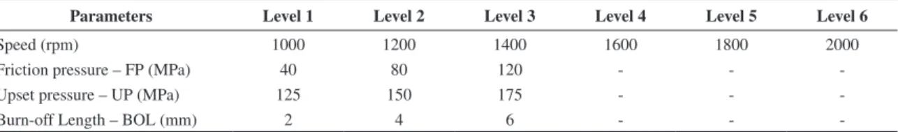
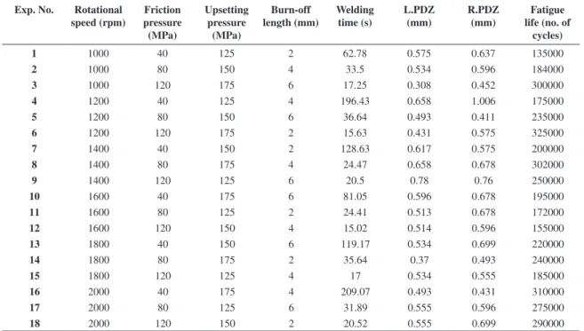
In this study, the experiments were conducted based on Taguchi L-18 orthogonal array16 . The frictional power, burn off length, upset power and rotational speed were the input parameters with three levels each. The selected welding parameters and their levels are listed in Table 2. For each experimental test condition two trials were performed. The average of the two trials was considered as the output of a test condition, in order to ensure the repeatability of the test result. The welded specimens are shown in Figure 3.
The welding time was recorded from the machine for both the specimens and the average was taken. Using one out of the two sets of specimens, the macrograph was prepared. The weld profiles were prepared by machining process, and cut into a cross section of 10 x 10 mm and polished with suitable abrasive and diamond paste. Weld samples were etched with 10% oxalic acid, an electrolyte, to state and increase the contrast of the fusion zone with the base metal. The macrograph of etched samples are shown in Figure 4a-d. The left partially deformed zone (L.PDZ) and right partially deformed zone (R.PDZ) were measured.
2.2.
Fatigue test
poor, incomplete, and uncertain systems. This grey-based Taguchi technique has been widely used in different fields of engineering to solve multi-response optimization problems. In order to apply the grey-based Taguchi method for multi-response optimization, the following seven steps were followed:
Step 1: S/N ratio for the corresponding responses was calculated using the following formula:
(i) Larger-the-better:
10 2
1
1 1
S / N ratio ( ) = –10 log
n
i ij
n = y
η
∑ (1)
Where n=number of replications yij=observed response value where i=1, 2, ....n; j=1, 2...k
This was applied for the problem where maximization of the quality characteristic of interest was sought. This was referred as the larger-the-better type problem.
(ii) Smaller - the – better:
2 10
1
1 S / N ratio ( ) = –10 log
n ij i
y n =
η
∑ (2)
This was termed as the smaller-the-better type problem where minimization of the characteristic was intended.
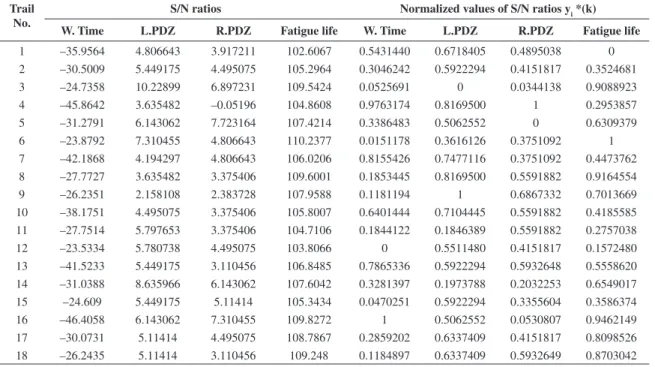
The S/N ratios for a given response like fatigue strength (larger-the-better) and welding time, partially deformed zone (left & right) (smaller-the-better) were calculated by using Equations 1 and 2, respectively. The computed S/N ratios for each quality characteristic are shown in Table 4
Step 2: Normalization is a transformation performed on a single data input to distribute the data evenly and scale it in to an acceptable range for further analysis. Therefore, the normalization of original sequence of these four responses was done. As fatigue life follows Larger - the – better criterion (LB) normalization was done by Equation “1”.
( )
( )
( )
min( )
( )
*max min
i
yi k yi k
y k
yi k yi k
−
= − (3)
Where yi*(k) is the normalized data, i.e. after grey relational generation, yi(k) is the kth response of the ith
experiment, min yi(k) is the smallest value of yi(k) for the kth response, and max y
i(k) is the largest value of yi(k) for
the kth response.
Welding time and partially deformed zone (left & right) follows the smaller - the – better (SB) criterion. Figure 1. Friction welding weld cycle.
Figure 2. Friction welding machine.
Figure 3. Friction Welded joints.
Table 1. Chemical composition of the Base material (wt. %).
Elements Si Mn P S Cr Ni Mo C Cu
Composition (%) 0.374 1.522 0.018 0.004 19.893 25.557 4.124 0.018 1.650
Table 2. Welding parameter levels.
Parameters Level 1 Level 2 Level 3 Level 4 Level 5 Level 6
Speed (rpm) 1000 1200 1400 1600 1800 2000
Friction pressure – FP (MPa) 40 80 120 - -
-Upset pressure – UP (MPa) 125 150 175 - -
-Burn-off Length – BOL (mm) 2 4 6 - -
-as per the ASTM E647-04 standard. The fatigue tested specimens are shown in Figure 5. The experimental data is tabulated in Table 3.
3. Methodologies and Implementations
3.1.
Grey relational analysis
Figure 4. Macrograph of the welded joint.
Table 3. Experimental results.
Exp. No. Rotational speed (rpm)
Friction pressure (MPa)
Upsetting pressure
(MPa)
Burn-off length (mm)
Welding time (s)
L.PDZ (mm)
R.PDZ (mm)
Fatigue life (no. of
cycles)
1 1000 40 125 2 62.78 0.575 0.637 135000
2 1000 80 150 4 33.5 0.534 0.596 184000
3 1000 120 175 6 17.25 0.308 0.452 300000
4 1200 40 125 4 196.43 0.658 1.006 175000
5 1200 80 150 6 36.64 0.493 0.411 235000
6 1200 120 175 2 15.63 0.431 0.575 325000
7 1400 40 150 2 128.63 0.617 0.575 200000
8 1400 80 175 4 24.47 0.658 0.678 302000
9 1400 120 125 6 20.5 0.78 0.76 250000
10 1600 40 175 6 81.05 0.596 0.678 195000
11 1600 80 125 2 24.41 0.513 0.678 172000
12 1600 120 150 4 15.02 0.514 0.596 155000
13 1800 40 150 6 119.17 0.534 0.699 220000
14 1800 80 175 2 35.64 0.37 0.493 240000
15 1800 120 125 4 17 0.534 0.555 185000
16 2000 40 175 4 209.07 0.493 0.431 310000
17 2000 80 125 6 31.89 0.555 0.596 275000
Accordingly, the normalization of these responses was done using Equation “4”.
( )
max( )
( )
min( )
( )
*max min
i
yi k yi k
y k
yi k yi k
−
= − (4)
The S/N ratio values were normalized by using Equations 3 and 4 and calculated normalized values are presented in the same Table 4.
Step 3: The grey relational coefficient was calculated as
( )
min( )
max0 max'
i k
i k
∆ + ϖ∆
ε =∆ + ϖ∆ (5)
where the grey relational coefficient of the ith experiment for
the kth response is ∆
oi (k) =||y*o(k) - y*i(k)||, i.e. , absolute of
the difference between y*o(k) and y*i(k) , y*o(k) is the ideal or reference sequence, ∆max = maxi maxk||y*o(k) - y*i(k)|| is the
largest value of ∆oi , and ∆min = maxi maxk ||y*o(k) - y*i(k)|| is the smallest value of ∆oi , and ω(0≤ω≤ 1) is the distinguish
coefficient.
From the data in Table 4, the grey relational co-efficient for the normalized S/N ratio values was calculated by using Equation 5. The value for ξ∆max is taken as 0.6, 0.2, 0.1 and 0.1 for fatigue strength, welding time, partially deformed zone left and right respectively in Equation 5. The results are given in Table 5
Step 4: The grey relational grade (Γi) was calculated by averaging the grey relational coefficients corresponding to each experiment.
( )
11 Q
i =i k
Γ = ∑ (6)
Where, Q is the total number of responses. A high grey relational grade corresponds to intense relational degree between the given sequence and the reference sequence. The reference sequence, y*o (k), represented the best process sequence; therefore, higher grey relational grade meant that the corresponding parameter combination was closer to the optimal setting. The grey relational grade can be computed by Equation 6. Finally, the grades were considered for optimizing the multi response parameter design problem. The results are given in the Table 5.
Step 5: The optimal factor and its level combination were determined. The higher grey relational grade implied the better product quality; therefore, on the basis of grey relational grade, the factor effect can be estimated and the optimal level for each controllable factor can also be determined. For example, to estimate the effect of factor ‘i’, we calculated the average of grey grade values (AGV) for each level ‘j’, denoted as AGVij, and then the effect, Ei is defined as:
(
)
(
)
max min
Ei=− AGVij AGVij (7)
If the factor i is controllable, the best level j*, is determined by
Table 4. S/N ratio values and normalized S/N ratio values.
Trail No.
S/N ratios Normalized values of S/N ratios yi *(k) W. Time L.PDZ R.PDZ Fatigue life W. Time L.PDZ R.PDZ Fatigue life
1 –35.9564 4.806643 3.917211 102.6067 0.5431440 0.6718405 0.4895038 0 2 –30.5009 5.449175 4.495075 105.2964 0.3046242 0.5922294 0.4151817 0.3524681 3 –24.7358 10.22899 6.897231 109.5424 0.0525691 0 0.0344138 0.9088923 4 –45.8642 3.635482 –0.05196 104.8608 0.9763174 0.8169500 1 0.2953857 5 –31.2791 6.143062 7.723164 107.4214 0.3386483 0.5062552 0 0.6309379 6 –23.8792 7.310455 4.806643 110.2377 0.0151178 0.3616126 0.3751092 1 7 –42.1868 4.194297 4.806643 106.0206 0.8155426 0.7477116 0.3751092 0.4473762 8 –27.7727 3.635482 3.375406 109.6001 0.1853445 0.8169500 0.5591882 0.9164554 9 –26.2351 2.158108 2.383728 107.9588 0.1181194 1 0.6867332 0.7013669 10 –38.1751 4.495075 3.375406 105.8007 0.6401444 0.7104445 0.5591882 0.4185585 11 –27.7514 5.797653 3.375406 104.7106 0.1844122 0.1846389 0.5591882 0.2757038 12 –23.5334 5.780738 4.495075 103.8066 0 0.5511480 0.4151817 0.1572480 13 –41.5233 5.449175 3.110456 106.8485 0.7865336 0.5922294 0.5932648 0.5558620 14 –31.0388 8.635966 6.143062 107.6042 0.3281397 0.1973788 0.2032253 0.6549017 15 –24.609 5.449175 5.11414 105.3434 0.0470251 0.5922294 0.3355604 0.3586374 16 –46.4058 6.143062 7.310455 109.8272 1 0.5062552 0.0530807 0.9462149 17 –30.0731 5.11414 4.495075 108.7867 0.2859202 0.6337409 0.4151817 0.8098526 18 –26.2435 5.11414 3.110456 109.248 0.1184897 0.6337409 0.5932649 0.8703042
(
)
* max
j = AGVij (8)
From the value of grey relational grade in Table 5, by using Equations 7 and 8, the main effects are tabulated in Table 6 and the factor effects are plotted in Figure 6.
Step 5: ANOVA was performed for identifying the significant factors.
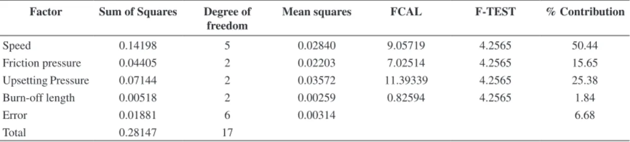
The main purpose of the analysis of variance (ANOVA) was to apply a statistical method to identify the effect of individual factors. Results from ANOVA would determine very clearly the impact of each factor on the process results. The Taguchi experimental method could not judge the effect of individual parameters on the entire process; thus, the percentage of contribution using ANOVA was used to compensate this effect. The total sum of the squared deviations SST was decomposed into two sources: the sum of the squared deviations due to each process parameter and the sum of the squared error. The percentage contribution by each of the process parameter in the total sum of the squared deviations SST can be used to evaluate the importance of the process parameter change on the performance characteristics. Usually, the change of the process parameter has a significant effect on the performance characteristic when the ‘F’ value is large.
The results of ANOVA are given in Table 7. From ANOVA, it is clear that rotational speed (50.44%) influences more on welding followed by upsetting pressure (25.38%), friction pressure (15.65%), and burn-off length (1.84%).
3.2.
Desirability approach
The desirability function approach to optimize multiple equations simultaneously was originally proposed by Harrington. Essentially, the approach is to translate the functions to a common scale (0, 1), combine them using the geometric mean and optimize the overall metric. There are many statistical techniques like overlaying the contours plot for each response, constrained optimization problems and desirability approach for solving multiple response problems. The desirability method is recommended due to its simplicity, availability in the software, flexibility in weighting and giving importance for individual response. Solving such multiple response optimization problems using this technique involves using a technique for combining multiple responses into a dimensionless measure of performance called the overall desirability function. The desirability approach involves transforming each estimated response, Yi, into a unit less utility bounded by 0<di<1, where a higher ‘di’ value indicates that response value Yi is more desirable, if di=0 this means a completely undesired
Table 5. Grey relational co-efficient and grey grade values.
Trail No
Grey relational co-efficient Grey grade
W. Time L.PDZ R.PDZ Fatigue life
1 0.304481 0.233558 0.163801 0.375 0.325632
2 0.22337 0.196939 0.146024 0.48095 0.36754
3 0.174302 0.090909 0.093845 0.868171 0.574239
4 0.894124 0.353294 1 0.459906 0.590098
5 0.232193 0.168423 0.090909 0.619155 0.443865
6 0.168793 0.13543 0.137952 1 0.661097
7 0.520214 0.283858 0.137952 0.520551 0.458555
8 0.197111 0.353294 0.184907 0.877777 0.619909
9 0.184863 1 0.241974 0.667681 0.561779
10 0.357235 0.256703 0.184907 0.507854 0.420321
11 0.19693 0.109247 0.184907 0.453071 0.340644
12 0.166667 0.182198 0.146024 0.415872 0.315679
13 0.483715 0.196939 0.197342 0.574637 0.480953
14 0.229395 0.110788 0.111511 0.634855 0.449022
15 0.173464 0.196939 0.130815 0.48334 0.357472
16 1 0.168423 0.095518 0.917733 0.777034
17 0.218799 0.214473 0.146024 0.759352 0.535421
18 0.184927 0.214473 0.197342 0.822261 0.571523
Table 6. Main effects on grey grades.
Factor/ level 1 2 3 4 5 6 Difference Rank Optimum
Levels
response. In order to apply the desirability approach method for multi-response optimization, the following seven steps were followed:
Step 1: The individual desirability index (di) for the corresponding responses was calculated using the following Equations 9 and 10. There were different forms of the desirability functions according to the response characteristics.
The Larger-the better
min min min max max min min 0,
, , 0
1, j r j i j j y y y y
d y y y r
y y y y ≤ − = ≤ ≤ − ≥ ≥ (9)
The value of ‘yj’ was expected to be the larger the better. When the ‘y’ exceeded a particular criteria value, which can be viewed as the requirement, the desirability value equaled to 1; if the ‘y’ was less than a particular criteria value, which was unacceptable, the desirability value equaled to 0.
The Smaller-the better
min max min max min max min 1,
, , 0
0, j r j i j j y y y y
d y y y r
y y y y ≤ − = ≤ ≤ − ≥ ≥ (10)
The value of ‘yj’ was expected to be the smaller the better. When the ‘y’ was less than a particular criteria value, the desirability value equaled to 1; if the ‘y’ exceeds a particular criteria value, the desirability value equaled to 0.
The individual desirability (di) was calculated for all the responses depending upon the type of quality characteristics. The main objectives of this work are minimization of welding time, width of the partially deformed zone (left & right) and maximization of fatigue strength. According to this objective the responses were considered. The larger the better type and the smaller the better type were selected for this study. The values of computed individual desirability for each quality characteristics using the Equations 9 and 10 are presented in Table 8.
Step 2: The composite desirability (dG) was computed. The individual desirability index of all the responses can be combined to form a single value called composite desirability (dG) by the following Equation 11.
(
1 2)
1w 2w ... wi w
G i
d = d ×d d (11)
The composite desirability values (dG) were calculated using equation 11. The weightage for responses were based on assumption of fatigue strength (0.6), welding time (0.2) and Left partially deformed zone (0.1) and Right partially deformed zone (0.1). Finally, these values were considered for optimizing the multi-response parameter design problem and the calculated results are given in the Table 8.
Step 3: The optimal parameter and its level combination were determined. The higher composite desirability value implied better product quality. Therefore, on the basis of the composite desirability (dG), the parameter effect and the optimum level for each controllable parameter were estimated. For examples, to estimate the effect of factor ‘i’, we calculated the composite desirability values (CDV) for each level ‘j’, denoted as CDVij, and then the effect, Ei is defined as:
( )
( )
max – min
i ij ij
E = CDV CDV (12)
If the factor i is controllable, the best level j*, is determined by
( )
* maxj ij
j = CDV (13)
From the value of composite desirability in Table 8, by using Equations 12 and 13, the main parameter effects are tabulated in Table 9 and the factor effects are plotted in Figure 7.
Step 4: ANOVA was performed for identifying the significant parameters. ANOVA established the relative significance of parameters. The calculated total sum of square values was used to measure the relative influence
Table 7. Results of ANOVA on grey grade.
Factor Sum of Squares Degree of freedom
Mean squares FCAL F-TEST % Contribution
Speed 0.14198 5 0.02840 9.05719 4.2565 50.44
Friction pressure 0.04405 2 0.02203 7.02514 4.2565 15.65 Upsetting Pressure 0.07144 2 0.03572 11.39339 4.2565 25.38
Burn-off length 0.00518 2 0.00259 0.82594 4.2565 1.84
Error 0.01881 6 0.00314 6.68
Total 0.28147 17
of the parameters. Using the composite desirability value, ANOVA was formulated for identifying the significance of the individual factors.
The results of ANOVA are given in Table 10. From ANOVA, it was clear that rotational speed (37.90%) influenced more on welding followed by upsetting pressure (22.60%), friction pressure (25.60%), and burn-off length (6.94%).
3.3.
Genetic algorithm
Genetic algorithms (GAs) are well known types of evolutionary computation methods and they have been adapted for large number of applications in different
areas. The GAs differ from most optimization techniques because of their global searching from one population of solutions rather than from one single solution. It is a heuristic technique inspired by the natural biological evolutionary process comprising of proper selection of, crossover, mutation, etc. The evolution starts with a population of randomly generated individuals in first generation. In each generation, the fitness of every individual in the population is evaluated, compared with the best value, and modified (recombined and possibly randomly mutated), if required, to form a new population. The new population is then used in the next iteration of the algorithm. The algorithm terminates, when either a maximum number of generations has been produced or a satisfactory fitness level has been reached for the population. The general schema (Figure 8) of GA may be summed up as follows
This study is to determine the set of optimal parameters of friction welding process to ensure minimum weld time, minimum partially deformed zone (Left and Right) and after satisfying the condition of maximum fatigue strength. Mathematical formulation of the problem was carried out to reach the desired output responses. The above constrained optimization problem can mathematically be stated as follows:
Figure 7. Factor effects on grade values.
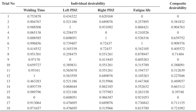
Table 8. Desirability values and composite desirability values.
Trial No Individual desirability Composite
desirability
Welding Time Left PDZ Right PDZ Fatigue life
1 0.753878 0.434322 0.620168 0 0
2 0.904767 0.521186 0.689076 0.257895 0.381832
3 0.988508 1 0.931092 0.868421 0.904763
4 0.065138 0.258475 0 0.210526 0
5 0.888585 0.608051 1 0.526316 0.639752
6 0.996856 0.739407 0.72437 1 0.909376
7 0.414532 0.345339 0.72437 0.342105 0.405572
8 0.951301 0.258475 0.551261 0.878947 0.71404
9 0.97176 0 0.413445 0.605263 0
10 0.659727 0.389831 0.551261 0.315789 0.388091
11 0.95161 0.565678 0.551261 0.194737 0.312639
12 1 0.563559 0.689076 0.105263 0.227046
13 0.463283 0.521186 0.515966 0.447368 0.469037
14 0.893739 0.868644 0.862185 0.552632 0.663112
15 0.989796 0.521186 0.757983 0.263158 0.39748
16 0 0.608051 0.966387 0.921053 0
17 0.913064 0.476695 0.689076 0.736842 0.711135
18 0.971657 0.476695 0.515966 0.815789 0.721092
Table 9. Main effects on desirability analysis.
Factor/level 1 2 3 4 5 6 Difference Rank Optimum
Levels
( )
(
)
(
)
( )
( )
(
)
( )
(
( )
( )
( )
)
2 2 exp exp 2 2 exp expf t w t
t t
p t p t
t t
c F F c w w
Of i
F w
c P L P L c P R P R
P L P R
− − =+ − − + + (14) Where,
• Of(i) -Value of the objective function at the “i” experiment;
• Ft - Target (desirable) value for fatigue life;
• Fexp (i) - Experimental value for the fatigue life at the “i” experiment;
• Wt - Target value for the welding time;
• Wexp (i) - Experimental value for the welding time at the“i” experiment;
• P(L) -Target value for the left partially deformed zone;
• P(L)exp (i) - Experimental value for the left partially
deformed zone; at the “i” experiment;
• P(R)-Targetvaluefortherightpartiallydeformed zone;
• P(R)exp (i) - Experimental value for the right partially
deformed zone at the “i”experiment;
• cf(0.6), cw(0.2) and cp(0.1) -Weights that give different status (importance) to each response
Subject to the condition that fatigue life takes the maximum value and welding time and partially deformed zone (left and right) within the range of input parameters.
Regression analysis was carried out using Minitab-14 software using the experimental data collected as per the experiments conducted (Table 3). Output responses were expressed in a coded form as a linear function of process parameters, namely S, FP, UP and BOL, represented by X1, X2 X3 and X4, respectively.
( )
( )
( )
( )
exp 129103 37.1 1 563 2
1600 3 4700 4
F codec X X
X X
=
− + +
+ + (15)
( )
( )
( )
( )
exp 125 0.0217 1 1.44 2
0.100 3 0.79 4
W codec X X
X X
=
+ −
+ + (16)
( )
( )
( )
( )
( )
exp 0.939 0.000003 1 0.00073 1
0.00253 3 0.0085 4
P L X X
X X
=+ −
− + (17)
( )
( )
( )
( )
( )
exp 1.20 0.000028 1 0.000810 2
0.00308 3 0.0025 4
P R X X
X X
=
− −
− − (18)
The coded and un-coded values of the variables can be related as given below
(
)
(
max min 2)
1
max min
S S S
X
S S
− +
= − (19)
(
)
(
max min 2)
2
max min
FP FP FP
X
FP FP
− +
=
− (20)
(
)
(
max min 2)
3
max min
UP UP UP
X
UP UP
− +
= − (21)
(
)
(
max min 2)
4
max min
BOL BOL BOL
X
BOL BOL
− +
= − (22)
Analysis was carried out at a confidence level of 95%. The un-coded form of the response equations was found to be as follows:
( )
( )
( )
(
)
expun-coded 146020 0.0371
7.04 32 1177
F S
FP UP BOL
=
− +
+ + + (23)
( )
( )
( )
(
)
expun-coded 125.6 0.0000217 0.018
0.002 0.1975
W S FP
UP BOL
=
+ −
+ + (24)
Table 10. Results of ANOVA on desirability analysis.
Factor Sum of Squares Degree of freedom
Mean squares FCAL F-TEST % Contribution
Speed 0.60605 5 0.12121 6.73290 4.2565 37.90
Friction Pressure 0.41292 2 0.20646 11.4683 4.2565 25.82 Upsetting Pressure 0.36128 2 0.18064 10.0339 4.2565 22.60
Burn-off length 0.11092 2 0.05546 3.08072 4.2565 6.94
Error 0.10802 6 0.01800 6.75
Total 1.59920 17
( )
( )
( )
( )
(
)
exp 0.9375 0.000000003 0.0000092
0.000050 0.0021
P L S FP
UP BOL
=+ −
− + (25)
( )
( )
( )
( )
(
)
exp 1.22 0.000000028 0.000010
0.000062 0.00063
P R S FP
UP BOL
=
− −
− − (26)
A binary-coded genetic algorithm (GA) in MATLAB 7.0 was used to solve the optimization problem presented. Inside the experimental space, the GAs chose, randomly, the initial welding setup, i.e., the parameters’ values of the first experiment within the input parameter range i.e. Speed (1000-2000rpm), Friction pressure (40-120Mpa), Upsetting pressure (125-175Mpa) and BOL (2-6mm). After it (the first exp.) was done, its response characteristics were measured and fed into the GAs. Then, based on the previous information, the algorithm chose another setup, carried out the experimentation and its data were again fed into the algorithm. This process was continued until the optimum was found, i.e., until the objective function (Equation 15) reached its minimum. In the GA, the population size, crossover rate and mutation rate were important factors in the performance of the algorithm. In this work, the GA parameters selected were as follows, Population size (100), Number of generations (50), Probability of mutation (0.008), Cross over rate (0.5) and Selection function (Roulette).
4. Results and Discussions
Investigations were carried out already to assess the relationship of microstructure/property relationships of similar and dissimilar joints of stainless steel by various welding processes18-20. Due to the difficulties associated with conventional way of optimization, we used evolutionary computational techniques to get the optimized parameters. Based on the preliminary trails for the grey relational and desirability analysis we identified that the process parameters namely rotational speed, friction pressure,
upsetting pressure significantly influenced fatigue life, welding time and partially deformed zone (left& right) while burn-off-length had relatively small influence. The initial parameters were chosen based on the initial trails and the predicted parameters were selected based on the obtained result from grey relational and desirability analysis. The friction welding was performed on predicted parameters and the fatigue life, welding time, partially deformed zone (left & right) were measured and compared with the initial set of parameters output values. The predicted values were in good agreement with the initial values for both the models. The least percentage of errors was obtained for initial and predicted parameter output values.
Table 11 reflects the satisfactory results of confirmatory experiment. From Table 11 it is seen that, the predicted input parameters had better fatigue life, lower welding time and partially deformed zone (left & right). Similarly confirmation test was conducted for the outcomes of desirability analysis. The predicted parameters were found to be better when compared to initial parameters. The validation results demonstrated that the prediction analysis results were quite accurate as the percentages of error in prediction were in a good agreement. The parameters were optimized using binary-coded genetic algorithm (GA) in MATLAB 7.0 software. The properties to be optimized were welding time, partially deformed zone in the left, partially deformed zone in the right and fatigue life. The processed joint was further investigated by microstructure analysis and fracture surface of the fatigue tested sample through SEM analysis. The microstructures of the joint are presented in Figure 9a-c. Figure 9a, shows the well defined grain boundaries and Figure 9b it is easily distinguished the weld zone and PDZ. The weld side grains are finer when compared to the PDZ. From Figure 9c, it is observed that the material flow direction from the inner side of the contact surface to the outer boundary.
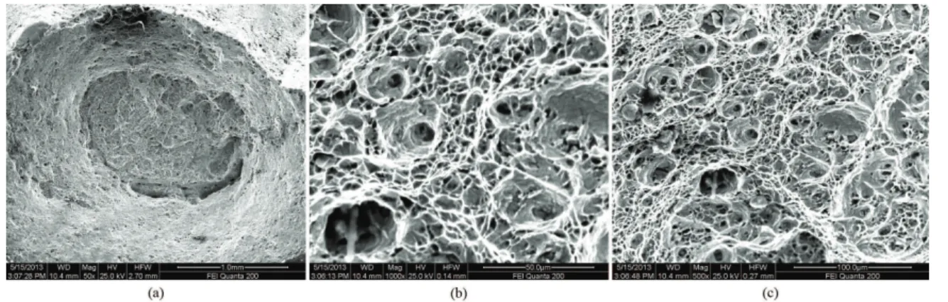
The fatigue fractured surfaces are analyzed through SEM and its structures are presented in Figure 10a-c.
Table 11. Results of confirmatory experiment (Grey relational).
Rotational Speed
FP UP BOL Fatigue life W. time L-PDZ R-PDZ
Initial parameter 2000 40 175 4 310000 209.07 0.493 0.431 Predicted parameter 2000 40 175 4 312437 202.2 0.475 0.416
Error(%) 0.78 3.58 3.65 3.48
From Figure 10a shows the fatigue crack propagated and the nature fracture took place. The fatigue crack fracture exhibits transgranularly under room temperature. From Figure 10b, c, the cleavage-type fractures were observed and also finer dimples are presented.
Since fatigue life was one of the important outputs for determining the life period of the weld, it was given more weightage for optimization of this work. Fatigue life was given a weightage of 0.6, welding time of 0.2 and the remaining properties such as L.PDZ, R.PDZ of 0.1 each. The optimal values of process parameters obtained by the GA are shown in Table 12.
The near optimum values of speed – 2000 rpm, FP – 120 MPa, UP – 175 MPa and BOL – 6 mm were selected for confirmation test. The result of the confirmation test is shown in Table 13.
5. Conclusions
The following important conclusions were drawn: • Theoptimizationoffrictionweldingparametersby
grey relational analysis, desirability approach and genetic algorithm was found to be successful; • BasedonANOVAresults,ithasbeenprovedthatboth
the grey relational and desirability approach analyses were accurate techniques to optimize the friction welding of super austenitic stainless steel joints;
• Greyrelationalanalysistechniqueperformedbetter in terms of predicting optimum welding parameters compared to desirability function analysis;
• TheoptimizedvaluesoftheparametersbyGenetic algorithm were;
• Speed – 1998.98 rpm; FP – 119.69 MPa; UP – 174.42 MPa; Burn-off Length – 5.99 mm; • For the optimized parameters, the friction welds
were processed and joints exhibited higher fatigue life. There was a good agreement between the theoretically predicted and experimentally obtained values of fatigue life, welding time, L.PDZ and R.PDZ. These computational techniques are the best suited for the optimization of friction welding parameters;
• Cleavage-typefractureswereoccurredinthefatigue tested samples.
Acknowledgements
We would like to express and convey our gratitude to Dr. K. Prasad Rao, Professor, Department of Metallurgical and Materials Engineering, for offering us the distinguished opportunity to use the friction welding Machine at the Indian Institute of Technology Madras, Chennai-600 025, TamilNadu, India.
Table 12. Optimum parameter values.
Speed (rpm) Frictional Pressure (MPa) Upsetting Pressure (MPa) Burn-off Length (mm)
1998.98 119.69 174.42 5.99
Table 13. Output values corresponding to optimum parameter values.
Welding time (s) L.PDZ (mm) R.PDZ (mm) Fatigue life (No of cycles)
47.27 0.481 0.437 310749
References
1. Li W-Y, Yu M, Li J, Zhang G and Wang S. Characterizations of 21-4N to 4Cr9Si2 stainless steel dissimilar joint bonded by electric- resistance-heat-aided friction welding. Journal
of Materials and Design. 2009; 30:4230-4235. http://dx.doi.
org/10.1016/j.matdes.2009.04.032
2. Sahin M. Evaluation of the joint-interface properties of austenitic-stainless steels (AISI 304) joined by friction welding.
Journal of Materials and Design. 2007; 28:2244-2250. http://
dx.doi.org/10.1016/j.matdes.2006.05.031
3. Dey HC, Ashfaq M, Bhaduri AK and Prasad Rao K. Joining of titanium to 304L Stainless steel by friction welding. Journal of
Materials Processing Technology. 2009; 209:5862-5870. http://
dx.doi.org/10.1016/j.jmatprotec.2009.06.018
4. Sahin M. Simulation of friction welding using a developed computer program. Journal of Materials Processing
Technology. 2004; 153-154:1011-1018. http://dx.doi.
org/10.1016/j.jmatprotec.2004.04.287
5. S a t h i y a P, A b d u l J a l e e l M Y a n d K a t h e r a s a n D . Optimization of laser butt welding Parameters with multiple performances characteristic. Journal of optics & laser
Technology. 2011; 43:660-673.
6. Benyounis KY and Olabi AG. Optimization of different welding processes using statistical and numerical approaches.
Journal of Advances in Engineering Software. 2008;
39:483-496. http://dx.doi.org/10.1016/j.advengsoft.2007.03.012 7. Sathiya P, Aravindan S, Noorul Haq A, Paneerselvam K.
Optimization of friction welding parameters using evolutionary computational techniques. Journal of Materials Processing
Technology. 2009; 209:2576-2584. http://dx.doi.org/10.1016/j.
jmatprotec.2008.06.030
8. Correia DS, Gonçalves CV, Junior SSC and Ferraresi VA. GMAW Welding Optimization Using Genetic Algorithms.
Journal of the Brazilian Society of Mechanical Sciences and
Engineering. 2004; 26:167-878. http://dx.doi.org/10.1590/
S1678-58782004000100005
9. Dey V, Pratihar DK, Datta GL, Jha MN, Saha TK and Bapat AV. Optimization of bead geometry in electron beam. Journal
of Materials Processing Technology. 2009; 209:1151-1157.
http://dx.doi.org/10.1016/j.jmatprotec.2008.03.019
10. Paventhan R, Lakshminarayanan PR and Balasubramanian V. Optimization of Friction Welding Process Parameters for Joining Carbon Steel and Stainless Steel. Journal of Iron And
Steel Research International. 2012; 19(1):66-71. http://dx.doi.
org/10.1016/S1006-706X(12)60049-1
11. Yousefieh M, Shamanian M and Saatchi A. Optimization of the pulsed current gas tungsten arc welding (PCGTAW) parameters for corrosion resistance of super duplex stainless steel (UNS S32760) welds using the Taguchi method. Journal of Alloys and
Compounds. 2010; 509:782-788. http://dx.doi.org/10.1016/j.
jallcom.2010.09.087
12. Gunaraj V and Murugan N. Application of response surface methodology for predicting weld bead quality in submerged arc welding of pipes. Journal of Materials Processing
Technology. 1999; 88:266-75. http://dx.doi.org/10.1016/
S0924-0136(98)00405-1
13. Rajakumar S, Muralidharan C and Balasubramanian V. Predicting tensile strength, hardness and corrosion rate of friction stir welded AA6061-T6 aluminium alloy joints.
Materials & Design. 2011; 32:2878-2890. http://dx.doi.
org/10.1016/j.matdes.2010.12.025
14. Sathiya P, Panneerselvam K and Abdul Jaleel MY. Optimization of laser welding process parameters for super austenitic stainless steel using artificial neural networks and genetic algorithm. Materials & Design. 2011; 32:1253-1261. 15. Konak A, Coit DW and Smith AE. Multi-objective optimization
using genetic algorithms: A tutorial. Reliable Engineering and
System Safety. 2006; 91:992-1007. http://dx.doi.org/10.1016/j.
ress.2005.11.018
16. Datta S, Bandyopadhyay A and Pal PK. Gery-based taguchi method for optimization of bead geometry in submerged arc bead-on-plate welding. International Journal of Advanced
Manufacturing Technology. 2007; 39- 11-12:1136-1143.
17. Deng J. Control problems of grey systems. Systems and control
Letter. 1982; 5:288-294.
18. Mohandas T, Madhusudhan Reddy G and Mohammad N. A comparative evaluation of gas tungsten and shielded metal arc welds of a ferritic stainless steel. Journal of Material
Processing Technology. 1999; 94:133-140. http://dx.doi.
org/10.1016/S0924-0136(99)00092-8
19. Murti KGK and Sundaresan S. Parameter optimization i n f r i c t i o n w e l d i n g d i s s i m i l a r m a t e r i a l s . M e t a l
Construction. 1983; 331-335.
20. Ramazan K and Orhan B. An investigation of microstructure/ properties relationships in dissimilar welds between martensitic and austenitic stainless steel. Materials and
Design. 2004; 25:317-329. http://dx.doi.org/10.1016/j.