ISSN 0104-6632 Printed in Brazil
Vol. 19, No. 03, pp. 307 - 317, July - September 2002
of Chemical
Engineering
NONLINEAR DYNAMIC MODELING
OF MULTICOMPONENT BATCH
DISTILLATION: A CASE STUDY
L.Jiménez
1*, M.S.Basualdo
2,3, J.C.Gómez
3,
L.Toselli
4and M.Rosa
41
Department of Chemical Engineering and Metallurgy, University of Barcelona, Martí i Franqués 1, 08028 Barcelona, Spain. E-mail:[email protected]
2
GIAIQ-Rosario Regional School, National Technical University, Zeballos 1341, 2000 Rosario, Santa Fe, Argentina
3
Department of Electronics, National University of Rosario, Riobamba 245 bis, 2000 Rosario, Santa Fe, Argentina
4
Villa María Regional School, National Technical University, Av. Universidad 450, 5900 Villa María, Argentina
(Received: October 6, 2001 ; Accepted: August 10, 2002)
Abstract - The aim of this work is to compare several of the commercial dynamic models for batch
distillation available worldwide. In this context, BATCHFRAC, CHEMCAD BATCH, and HYSYS.Plant software performances are compared to experimental data. The software can be used as soft sensors, playing the roll of ad-hoc observers or estimators for control objectives. Rigorous models were used as an alternative to predict the concentration profile and to specify the optimal switching time from products to slop cuts. The performance of a nonlinear model obtained using a novel identification algorithm was also studied. In addition, the strategy for continuous separation was revised with residue curve map analysis using Aspen SPLIT.
Keywords: batch distillation, residue curve map, soft sensor, inferential control, nonlinear identification.
INTRODUCTION
The increasing production of small-volume, high-value-added products has attracted increasing interest in batch production technologies. Although batch distillation typically consumes more energy than continuous distillation, operational flexibility is improved, and low capital investments are involved (Furlonge et al., 1999). Thus, since energy costs are not significant in the separation of specialties, batch distillation is often a cost-attractive alternative (Sørensen and Skogestad, 1996).
The development of accurate models of batch processes is a difficult problem for several reasons (Boston et al., 1981). First, information on product
batch distillation. The work by Henson and Seborg (1997) lists a number of simulation and experimental cases in which feedback controllers were used.
In this work, a nonlinear model-based strategy was developed with commercial software specifically suitable for modeling batch distillation operation. BATCHFRAC (Aspen Technology Inc, Cambridge, MA, USA), HYSYS.Plant® (AEA Technology, Calgary, Canada), and CHEMCAD BATCH (Chemstations Inc., Houston, TX, USA) performances were tested to evaluate whether their potentialities in other applications such as inferential control structure and/or soft sensor could be attractive.
PROBLEM STATEMENT
The process considered in this paper corresponds to a distillation column described in Nad and Spiegel (1987), from which the experimental data have been taken. The column has an internal diameter of 162 mm packed with Sulzer Mellapak 250Y. A packing height of 8.0 m was used, and the number of theoretical stages was measured with a standard method (chlorobenzene + ethylbenzene at total reflux). The column, including the reboiler and the condenser, has 20 theoretical stages. The volumetrically measured liquid hold ups of the column and the condenser were 0.015 m3 and 0.005 m3, respectively. The system was tested with a ternary mixture of n-heptane + cyclohexane + toluene. The initial charge, on a molar basis, was 39.40% for n-heptane, 40.70% for cyclohexane, and 19.90% for toluene. After 2.78 hours of operation, the steady state conditions of the column were reached. Then, the reflux ratio sequence and the switching time recommended by the authors were followed in order to compare the performance of the different software packages.
CLASSICAL APPROACH
Vapor-Liquid Equilibrium
A check of the accuracy of the estimation model of the physical properties is the key factor in succeeding in process simulation, and thus obtaining realistic equipment behavior (Carlson, 1996; Agarwall et al., 2001). The pure component vapor pressures were derived from the Antoine equation (Antoine, 1888). To avoid problems inherent in group contribution methods like UNIFAC in process
simulation (the interactions are computed from average values and do not consider the effect of groups that are not directly linked), the UNIQUAC (short for UNIversal QUAsi Chemical) method was selected (Abrams and Prausnitz, 1975). In this model, the liquid-phase activity coefficients can be individually differentiated in the combinatorial part, which includes the geometric significance for combining molecules of different shapes and sizes, and the residual part, which includes the energy parameters (Equations 1-3).
Comb Res
i i i
lnγ = γln + γln (1)
Comb i i
i
i i
i i
i
i i
ln = ln 1
x x
z
q ln 1
2
Φ Φ
γ + − −
Φ Φ − + −
θ θ
(2)
Res k ik
i j ji
i
j jk
j k
j ln = q 1 ln
θ τ
γ − θ τ −
θ τ
∑
∑∑
(3)where γi is the liquid-phase activity coefficient, xi is the liquid-phase molar fraction, and z is the coordination number (usually 10). The molecular volume fractions, Φi, and the molecular surface fractions, θi, are computed based on Equations 4 and 5.
i i i
j j j
x r r x
Φ ≡
∑
(4)i i i
j j j
x q q x
θ ≡
∑
(5)The molecular size (ri) and the molecular shape (qi) are computed from the group volume parameter (Rk) and the group surface area (Qk), as stated in Equations 6 and 7. υik is the number of groups of the kth type in the ith molecule
i
i k k
k
i
i k k
k
q =
∑
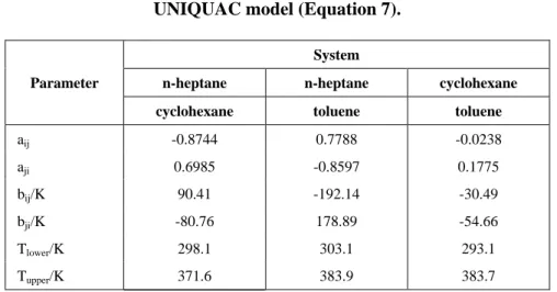
υ Q (7)τji (Equation 3) is the UNIQUAC interaction parameter that describes liquid-phase nonideality, while binary parameters a (aij≠aji) and b (bij≠bji) are determined from VLE and/or LLE data. The temperature-dependent parameters (Equation 8) were taken from the Aspen PLUS database. Ideal behavior was assumed for the vapor phase. To compare the results from different process simulators, the parameters shown in Table 1 were used.
ij
ij ij
b exp a
T
τ = +
(8)
Residue Curve Map Analysis
Residue curve maps (RCM) provide an understanding of the unit operations based on phase equilibrium (i.e., distillation) in a different way than process simulation. On the one hand, simulation results are snapshots of the equipment’s performance for selected conditions. On the other, these graphical tools provide fundamentals for multicomponent separations similar to the traditional McCabe-Thiele plots for binary mixtures. RCM are built based solely on the physical properties of the system: vapor-liquid equilibrium, liquid-liquid equilibrium, and solubility
data. In this context, RCM are applied to check, without intensive computing, the separation feasibility. The temperature always increases along a residue curve line, and the roles of the singular points (stable node, unstable node, or saddles) can be assigned according to the Doherty and Perkins rules (1979). The number and type of singular points (pure components and azeotropes) is unknown a priori. The singular points may be linked with distillation boundaries, thus stating the topology for the whole composition space. All calculations were performed with Aspen SPLIT.
The binary system n-heptane + toluene has a high purity binary azeotrope (0.99 mole fraction in n-heptane). This azeotrope is nonsensitive to pressure (0.975 molar at 10 atm.), and therefore pressure swing distillation is not a promising alternative for this separation. Applying the rules formulated by Doherty and Perkins, no ternary azeotrope exists in the system n-heptane + cyclohexane + toluene. The RCM was computed and is shown in Figure 1. The singular point detected acts as a saddle point, giving rise to a distillation boundary running from the azeotrope to the low-boiling component (cyclohexane) and thus leading to two regions in the ternary diagram. In the right region, where feed concentration is located, all distillation lines begin at cyclohexane and end at the high-boiling toluene, indicating that removal of toluene as a bottom product is feasible. In the small left region, all lines go from cyclohexane to n-heptane.
Table 1: Interaction parameters for the UNIQUAC model (Equation 7).
System
n-heptane n-heptane cyclohexane
Parameter
cyclohexane toluene toluene
aij -0.8744 0.7788 -0.0238
aji 0.6985 -0.8597 0.1775
bij/K 90.41 -192.14 -30.49
bji/K -80.76 178.89 -54.66
Tlower/K 298.1 303.1 293.1
Tol nC7
Cyclohexane
Toluene n-heptane
Distillation
boundary cC6
Binary azeotrope
Figure 1: Residue curve map for n-heptane + cyclohexane + toluene at 101.3 kPa.
Distillation Design Methods
In general, it is not possible to cross boundaries with distillation and recycle streams. It may be possible to cross distillation boundaries if unit operations other than distillation (i.e., liquid-liquid extraction, reactor, membrane, etc.) are considered or if the boundary is strongly curved. For all practical purposes it can be stated that, for homogeneous distillation, the whole separation sequence lies in the same distillation region. Computing a distillation column on a RCM is not difficult because the feed and the top and bottom products must lie in a straight line to satisfy the mass balance. The exact position of each point depends on its relative flowrate. In addition, both products must be on the same residue curve line.
Two preliminary design methods were used. The boundary value procedure (BV) was computed to assess the separation feasibility and to calculate the minimum reflux/reboil ratio for a fixed component recovery (99 mol %). BV performs calculations by starting at both ends of the column and computing towards the middle; a separation is feasible if the lines that illustrate the rectifying and the stripping concentration profiles intersect. The omega design procedure (Ω) optimizes the feed stage location by
studying the effect on the number of rectifying and stripping stages. The last method is only applicable for separations in which one of the products is a node (stable or unstable).
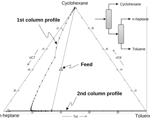
The results from BV and Ω methods for both approaches (remove first the light or the heavy component) are very similar, recovering pure cyclohexane, pure toluene, and the azeotrope. Figure 2 shows the concentration profiles for the second strategy, in which the second column is very close to the n-heptane + toluene axis.
PROCESS MODELING
A model for the system described by Nad and Spiegel (1987) was developed. HYSYS.Plant® and BATCHFRAC use rigorous calculations, with several methods available to integrate the differential equations, while CHEMCAD BATCH uses a pseudostationary model.
Initialization with HYSYS.Plant
reflux valve is opened until the stages have the experimental holdup; hence, the initial conditions can be reproduced. To model the start-up period, the reflux ratio is set to infinity, the heat duty is fixed, and the feed and product flowrates are set to zero. The predicted start-up period is 2.66 hours, a value with only a 4.3% deviation.
Initialization using BATCHFRAC
Initial conditions were fixed as the total reflux stationary values. Due to software limitations, no time considerations were implemented for the start-up period, and therefore it was reached instantaneously. To model the whole production period in a single run, the accumulator type, the feed-loading time, and the operational procedure (sequence of operational steps linked by the so-called stop criteria) were fixed. In this case, the reflux ratio was modified according to time considerations. Dump action for the different
fractions was continuous, and cut time switches were introduced between two operational steps.
The Pseudostationary Model of CHEMCAD BATCH
CHEMCAD BATCH models the discontinuous operation with the CC-BATCH module. The simulation of batch unit operations is performed as a sequence of pseudostationary states, in which each step begins with the final conditions of the previous one, and the calculations are performed linking a series of steady states. The option of having the same concentration in the still pot, plates, and condenser is adopted for the initialization period. During start-up, the conditions were set to total reflux. To calculate the production period, a set of thirty independent operating steps were necessary. Batch distillation was integrated with continuous operation with the use of tanks and time switches between certain operational steps.
Tol nC7
Cyclohexane
Toluene n-heptane
2nd column profile 1st column profile
Feed
Cyclohexane
n-heptane
Toluene
cC6
SIMULATION RESULTS
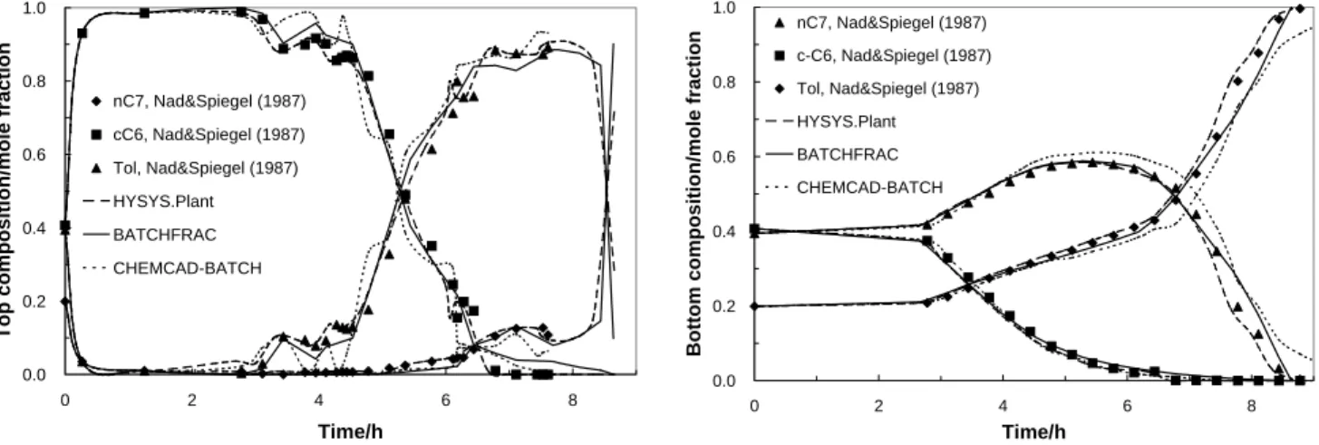
The results for top and bottom concentrations (Figures 3a and 3b) for the three models agree very well with the experimental data (∆x = 0.01-0.04,
∆xmax = 0.084, average percentage deviation = 2.5%, and maximum percentage deviation = 9.8%), especially CHEMCAD, which yields more accurate predictions. Thus, they are good candidates for acting as soft sensors either on- or off-line. This strategy is extremely useful for replacing on-line
analyzers, which are very expensive, and high maintenance and have significant time lags.
The predicted temperature is in good agreement with the experimental temperature ( T∆ = 1.5-2.5oC,
∆Tmax = 4.6oC, average percentage deviation = 1.4%, and maximum percentage deviation = 4.7%), as shown in Figures 4a and 4b. However, if the models are to be used as ad-hoc observers or estimators for control purposes, the temperature is the best variable for estimating the concentration in both top and bottom stages.
0.0 0.2 0.4 0.6 0.8 1.0
0 2 4 6 8
Time/h
Top composition/mole fraction
nC7, Nad&Spiegel (1987)
cC6, Nad&Spiegel (1987)
Tol, Nad&Spiegel (1987)
HYSYS.Plant
BATCHFRAC
CHEMCAD-BATCH
0.0 0.2 0.4 0.6 0.8 1.0
0 2 4 6 8
Time/h
Bottom composition/mole fraction
nC7, Nad&Spiegel (1987)
c-C6, Nad&Spiegel (1987)
Tol, Nad&Spiegel (1987)
HYSYS.Plant
BATCHFRAC
CHEMCAD-BATCH
Figures 3a and 3b: Dynamic behavior of top and bottom concentrations.
75 85 95 105
2 4 6 8
Time/h
Top temperature/
oC
Nad&Spiegel (1987)
HYSYS.Plant
BATCHFRAC
CHEMCAD-BATCH
90 95 100 105 110
2 4 6 8
Time/h
Bottom temperature/
oC
Nad&Spiegel (1987)
HYSYS.Plant
BATCHFRAC
CHEMCAD-BATCH
Figure 4a and 4b: Dynamic behavior of top and bottom temperatures.
( )
•
N
( )
( )
1 1− −
q A
q B
k
u
k
υ
k
y
NONLINEAR IDENTIFICATION METHODS
A Brief Review
In contrast to linear models that approximate the system around a given operating point, nonlinear models are able to describe the global behavior of the system over the entire operating range. One of the most frequently studied classes of nonlinear models is the Hammerstein models, which consists of the cascade connection of a static (zero-memory) nonlinearity and a linear time invariant (LTI) system (Ljung, 1999; Eskinat et al., 1991).
In this section, a noniterative algorithm for the estimation of Hammerstein models, which is based only on least square estimation, and singular value decomposition, is presented. The algorithm is then used to estimate a nonlinear model of the process. The data used for the identification are generated via simulation of a rigorous model of the column based on first principles, implemented with the commercial package HYSYS.Plant®, tuned to match the experimental data. As a result of the identification process, a reduced-order nonlinear model that is suitable for control design is obtained. For the purposes of comparison, the same data are used to estimate a state-space (linear) model of the column, using a subspace identification method (Viberg, 1995). Hammerstein Model Identification
A Hammerstein model is schematically depicted in Figure 5. The model can be described by the following nonlinear equation:
( )
( )
( )
( )
( )
( )
1
k 1 k k
1 r
i i k k
1 i 1 B q
y u =
A q
B q
= c g u
A q −
−
−
− =
= + υ
+ υ
∑
N(9)
where yk, uk, and υk are the system output, input, and disturbance at time k, respectively, gi(*) are nonlinear functions used to describe the nonlinear zero-memory subsystem N(*), and
( )
( )
1 1 n
1 n
1 1 m
1 m
A q 1 a q a q
B q b q b q
− − −
− − −
= + + +
= + +
(10)
with q-1 denoting the unit time-delay operator. It is assumed that the orders n, m, and s and the nonlinear functions gi(*) are known and that the goal is to estimate the parameters of the linear (a1,···, an, b1,···, bm) and nonlinear (c1,···, cr) subsystems from input-output data. A typical choice is to represent the nonlinear subsystem by a polynomial expansion. Equation (9) can be written as a (nonlinear) difference equation of the form
n r m
i
k j k j j i k j k
j 1 i 1 j 1
y a y − b c u −
= = =
= −
∑
+∑∑
+ υ (11)Now defining the vectors
(
)
T1 n 1 1 m 1 1 r m r
a , ,a , b c , , b c , , b c , , b c
θ = (12)
k k 1 k n k 1 k m
2 2 r r T
k 1 k m k 1 k m
( y , , y , u , , u ,
u , , u , , u , , u )
− − − −
− − − −
φ = − −
(13)
equation (11) can be written in linear regressor form as
T
k k k
y = φ θ + υ (14)
Finally, considering that an N-point input-output data set
{
y , uk k k 1}
N= is available for the identification, equation (14) can be written in matrix form asT
N N N
Y = Φ θ +V (15)
where
YN=(y1,···, yN)T, VN=(υ1,···, υN)T, and ΦN=(φ1,···, φN)T.
Least squares estimate ˆθ of parameter vector θ is given by
(
T)
1N N N N
ˆ − Y
θ = Φ Φ Φ (16)
1 1 1 2 1 r
2 1 2 2 2 r T
bc
m 1 m 2 m r
b c b c b c
b c b c b c
bc
b c b c b c
Θ = =
(17)
the parameter vector θ can then be written as
(
)
(
)
TT T
bc a , vec
θ = Θ (18)
where vec(Θbc) is the column vector obtained by stacking the columns of Θbc on top of each other. Estimates of vectors a and vec(Θbc) can then be obtained from estimate ˆθ in (16). Let â and
(
bc)
vec∧ Θ denote these estimates. The problem now is how to compute estimates of vectors b and c from estimate vec
(
bc)
∧
Θ .
From equation (11), it is clear that the parameterization in (9) is not unique, since any parameters αbj and α-1ci, for some nonzero scalar α will provide the same input-output equation (11). To avoid this identifiability problem, additional constraints must be imposed on the parameters. A standard procedure is to impose RER2=1 (or equivalently RFR2=1). Under this assumption the parameterization (9) is unique.
It is clear that, in the two-norm sense, the closest estimates ˆb and ˆc are such that they minimize the norm
( )
T(
)
2 T 2bc bc
F 2
ˆˆ ˆˆ ˆ
vec bc −vec∧ Θ = bc − Θ (19)
i.e.,
( )
T 2bc
F b,c
ˆ ˆ ˆ
b, c =argmin Θ −bc (20)
where RRF stands for the matrix Frobenius norm. The solution of this minimization problem is provided by the singular value decomposition of matrix Θˆbc. The mathematical details can be consulted elsewhere (Gómez and Basualdo, 2000). Identification Results
In this subsection the nonlinear identification algorithm described is employed to estimate a
Hammerstein model of the distillation process (Gómez and Basualdo, 2000). In this case, the input (u) of the system is the reflux ratio and the outputs (y1, y2, and y3) are the n-heptane, cyclohexane, and toluene concentrations, respectively. Since the sum of the three concentrations equals one, only two of them (e.g., y1 and y2) need to be estimated.
For the identification, r=3 terms were considered for the polynomial representation of the nonlinear subsystem. To select the "optimal" (in the mean square sense) order of polynomials A(q-1) and B(q-1), simulations were performed for the different combinations of n and m in the range from 2 to 5, and the combination giving the minimum mean-square error with the validation data was chosen as the optimal one. In this case the optimal orders were n=2 and m=3.
The rigorous HYSYS.Plant® model of the column was used to generate the extra data required to perform the identification properly. The interoperability facilities to transfer data were used to interface HYSYS-PI® and MATLAB® 5.1 (Mathworks Inc., Natick, MA, USA). The model was perturbed with a pseudorandom multilevel sequence, as shown in the top-left plot in Figure 6. The remaining plots of that figure show the real (solid lines) and the estimated (dotted lines) outputs using the nonlinear identification algorithm proposed in the paper.
For the purposes of comparison, the same data were used to estimate a (linear) state-space model using a subspace method. Subspace state-space system identification (4SID) methods have their origin in realization theory, developed in the sixties. These methods are able to deliver reliable state-space models of multivariable systems directly from input-output data, and they require only a modest computational complexity without the need for iterative optimization procedures (Basualdo and Gómez, 1999). The main computational tools are QR factorization and singular value decomposition, which can be implemented very efficiently from a numerical point of view (see Viberg, 1995 and the references therein).
The state-space model structure is given as
K 1 K K K
K K K K
x A·x B·u w
y C·x D·u v
+ = + +
= + +
(21)
where nx k
and vk are the process noise and the output measurement noise vectors, respectively, and where A, B, C, and D are the system matrices of appropriate dimensions to be estimated.
In this case, the N4SID algorithm by Van
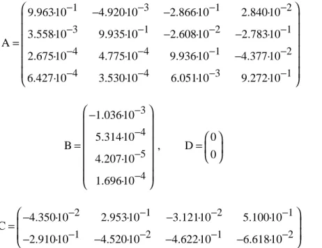
Overschee and de Moor (1994) was used for the estimation. The N4SID algorithm chooses automatically the best (in the mean-square sense) model order (default range is from 1 to 10). The resulting system matrix estimates are
1 3 1 2
3 1 2 1
4 4 1 2
4 4 3 1
9.963·10 4.920·10 2.866·10 2.840·10 3.558·10 9.935·10 2.608·10 2.783·10 A
2.675·10 4.775·10 9.936·10 4.377·10 6.427·10 3.530·10 6.051·10 9.272·10
− − − −
− − − −
− − − −
− − − −
− −
− −
=
−
(22)
3
4
5
4 1.036·10 5.314·10 B
4.207·10 1.696·10 − − − −
−
=
, D 0
0
=
(23)
2 1 2 1
1 2 1 2
4.350·10 2.953·10 3.121·10 5.100·10 C
2.910·10 4.520·10 4.622·10 6.618·10
− − − −
− − − −
− −
=
− − − −
(24)
The simulation results are also shown in Figure 6 (as dash-dotted lines). For the purposes of validation, a different data set was used to compute estimates of
the outputs of the identified system. Here again, there was very good agreement between the measured and the estimated outputs.
1 2 3 4
0 5 10 15
Refl
u
x rati
o
t/s·104
1 2 3 4
.2 .4 .6 .8
ycC6
t/s·104
1 2 3 4
.1 .2 .3 .4 .5
ytol
t/s·104
1 2 3 4
.2 .4 .6 .8
ynC7
t/s·104
CONCLUSIONS
In this work, a case study was considered to test the capabilities for modeling and interfacing experimental plant data with estimated values from three commercial software packages available worldwide (BATCHFRAC, CHEMCAD BATCH, and HYSYS.Plant). From the computational efficiency point of view, HYSYS.Plant and BATCHFRAC have the best performance. In particular, the use of InfoPLUS.21 in conjunction with its layered application (BATCHFRAC) has an important synergic effect. However, from the user-friendly point of view, CHEMCAD BATCH, and BATCHFRAC offer a simple way to model for less trained users.
In addition, by performing a simulation with a model that has been validated with plant data and implemented in the HYSYS.Plant® environment, it was possible to get enough data for applying identification techniques. Therefore, a methodology for the identification of nonlinear models of multicomponent batch distillation columns has been applied. As a result a reduced-order model which is especially suitable for control purposes, can be obtained.
NOMENCLATURE
4SID subspace-based state-space system identification
aij interaction parameter in the UNIQUAC equation, dimensionless
A, B, C, D state-space matrices of coefficients, defined in Eq. (19)
bij interaction parameter in the UNIQUAC equation, K-1
BV boundary value design
gi(*) nonlinear basis functions, defined in Eq. (9)
n number of inputs
N(*) static nonlinearity, defined in Eq. (9) m number of outputs
qi molecular shape
Qk group surface area RCM residue curve map ri molecular size
Rk group volume parameter T temperature, K
uk input vector
vk process noise vector wk output noise vector xi liquid molar fraction
xk state vector or state stacked vector yk output vector
z coordination number
Subscripts and Superscripts
Comb combinatorial i, j ith/jth component
k state-space variation in time or group type
max maximum Res residual T transposed
average value
Greek Symbols
∆ increment
φk regressor matrix, defined in Eq. 14
Φi molecular volume fractions
γi liquid-phase activity coefficient
τij interaction parameter in the UNIQUAC equation, dimensionless
i k
υ number of groups of the kth type in the ith molecule
θ parameter matrix, defined in Eq. 12
θi molecular surface fractions
Θbc block matrix, defined in Eq. 17
Ω omega design procedure
REFERENCES
Abrams, D. S. and Prausnitz, J. M., Statistical Thermodynamics of Liquid Mixtures: A New Expression for the Excess Gibbs Energy of Partly or Completely Miscible Systems, AIChE Journal, vol. 21, no. 1, pp. 116-128 (1975).
Agarwall, R., Li, Y. -K., Santollani, O., Satyro, M. A. and Vieler, A., Uncovering the Realities of Simulation. Part I, Chemical Engineering Progress, vol. 97, no. 5, pp. 42-52 (2001).
Basualdo, M. and Gomez, J. C., Subspace-Based Identification of Multicomponent Batch Distillation Processes, Computer-Aided Design for the 21st Century, Colorado, USA, pp. 157-162 (1999).
Boston, J. F., Britt, H. F., Jirapongphan, S. and Shah, V. B., An Advanced System for the Simulation of Batch Distillation Operation, Foundations of Computer-Aided Process Design FOCAPD‘81, Engineering Foundation, New York, USA, vol. 2, p. 203 (1981).
Carlson, E. C., Don’t Gamble with Physical Properties for Simulations, Chemical Engineering Progress, vol. 10, pp. 35-46 (1996).
Doherty, M. F. and Perkins, J. D., On the Dynamics of Distillation Processes-III. The Topological Structure of Ternary Residue Curve Maps, Chemical Engineering Science, vol. 34, pp. 1401-1414 (1979).
Eskinat, E., Johnson S. H. and Luyben, W. L., Use of Hammerstein Models in Identification of Nonlinear Systems, AIChE Journal, vol. 37, no. 2, pp 255-268 (1991).
Furlonge, H. I., Pantelides, C. C. and Sørensen, E., Optimal Operation of Multivessel Batch Distillation Columns, AIChE Journal, vol. 45, pp. 781-801 (1999).
Gómez, J. C. and Basualdo, M., Nonlinear Identification of Multicomponent Batch Distillation Processes. IFAC Symposium on Advanced Control of Chemical Processes ADCHEM 2000, Pisa, Italy, pp. 989-994 (2000). Henson, M. A. and Seborg, D., Nonlinear Process
Control. Prentice Hall PTR, London, UK (1997). Ljung, L., System Identification, Theory for the
User. 2nd Edition Prentice-Hall Int., NJ, USA (1999).
Luyben, W. L., Practical Distillation Control. Van Nostrand Reinhold, New York, USA (1992). Nad, M. and Spiegel, L., Simulation of Batch
Distillation with Experiment. Proceedings of the CEF’87: The Use of Computers in Chemical Engineering, Taormina, Italy, p. 737, (1987). Sørensen, E. and Skogestad, S., Comparison of
Inverted and Regular Batch Distillation, Chemical Engineering Science, vol. 51, no. 22, pp. 4949-4962 (1996).
Van Overschee, P. and de Moor, B., N4SID: Subspace Algorithms for the Identification of Combined Deterministic-Stochastic Systems, Automatica, vol. 30, no. 1, pp. 75-93 (1994). Viberg, M., Subspace-based Methods for the