www.ann-geophys.net/34/831/2016/ doi:10.5194/angeo-34-831-2016
© Author(s) 2016. CC Attribution 3.0 License.
Determination of errors in derived magnetic field directions in
geosynchronous orbit: results from a statistical approach
Yue Chen, Gregory Cunningham, and Michael Henderson
Los Alamos National Laboratory, Los Alamos, New Mexico, USA
Correspondence to:Yue Chen ([email protected])
Received: 24 December 2015 – Revised: 22 August 2016 – Accepted: 31 August 2016 – Published: 21 September 2016
Abstract.This study aims to statistically estimate the errors in local magnetic field directions that are derived from elec-tron directional distributions measured by Los Alamos Na-tional Laboratory geosynchronous (LANL GEO) satellites. First, by comparing derived and measured magnetic field di-rections along the GEO orbit to those calculated from three selected empirical global magnetic field models (including a static Olson and Pfitzer 1977 quiet magnetic field model, a simple dynamic Tsyganenko 1989 model, and a sophisti-cated dynamic Tsyganenko 2001 storm model), it is shown that the errors in both derived and modeled directions are at least comparable. Second, using a newly developed proxy method as well as comparing results from empirical models, we are able to provide for the first time circumstantial evi-dence showing that derived magnetic field directions should statistically match the real magnetic directions better, with averaged errors <∼2◦
, than those from the three empirical models with averaged errors>∼5◦
. In addition, our results suggest that the errors in derived magnetic field directions do not depend much on magnetospheric activity, in contrast to the empirical field models. Finally, as applications of the above conclusions, we show examples of electron pitch an-gle distributions observed by LANL GEO and also take the derived magnetic field directions as the real ones so as to test the performance of empirical field models along the GEO or-bits, with results suggesting dependence on solar cycles as well as satellite locations. This study demonstrates the valid-ity and value of the method that infers local magnetic field directions from particle spin-resolved distributions.
Keywords. Magnetospheric physics (energetic particles trapped; storms and substorms; instruments and techniques)
1 Introduction
It is well-known that energetic electrons in the Earth’s outer radiation belt – ranging from∼3 to 8 Earth radii (RE) – are highly dynamic and present storm-specific behaviors (e.g. Reeves et al., 2003; Chen et al., 2007b; Tu et al., 2014). Thus, monitoring, understanding, and forecasting the variations of outer-belt electrons are central topics for the space weather community. To address these topics, one basic imperative is to have long-term continuous observations with high qual-ity and good coverage over key areas, particularly regions close to the low-altitude boundary (i.e., the lower thermo-sphere and mesothermo-sphere where originally trapped electrons precipitate), the internal plasma boundary (i.e., the plasma-pause where wave-electron resonance prevails), as well as the high-altitude boundary (i.e., the magnetopause separating the enclosed drift shells from open ones). Among those regions, satellites in the geosynchronous orbit (GEO, a geo-equatorial circular orbit with geocentric distance of ∼6.6RE) play a unique role by monitoring the corridor through which sub-storm particles are injected into the inner magnetosphere, while radiation belt electrons can also be diffused outward towards the magnetopause.
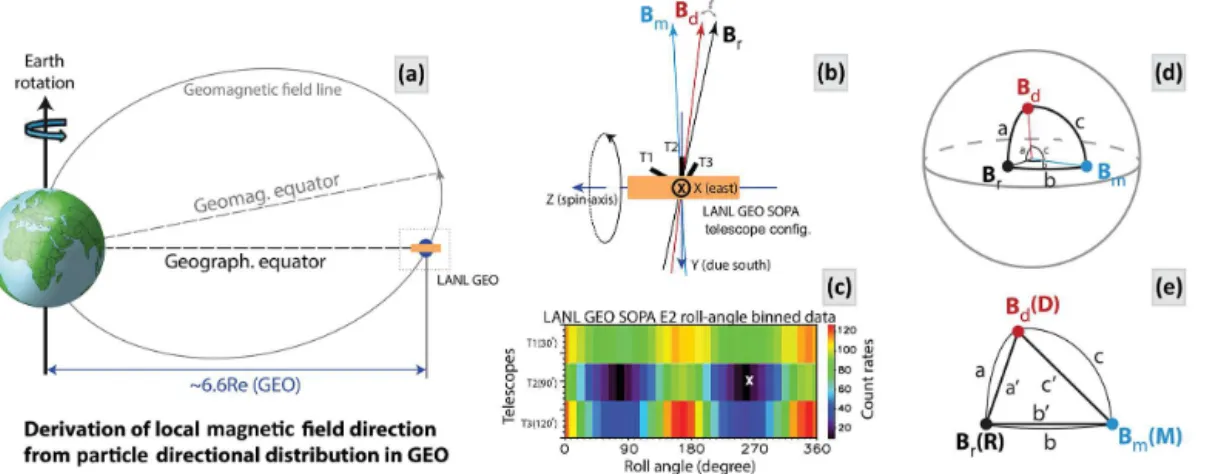
identify-Figure 1.LANL GEO satellites measure electron directional distributions.(a)Side view of the GEO orbit. A LANL GEO satellite is usually
close to but not exactly in the geomagnetic equator due to the tilted geomagnetic dipole field.(b)Rotation of the satellite platform allows the
three SOPA telescopes (T1, 30◦to the spin axisz; T2, 90◦, and T3, 120◦) to sample directional distributions of electrons; meanwhile, the unit
local magnetic field from the empirical model (Bmin blue), the one derived from electron distribution (Bdin red), and the real direction (Br
in black, if measured) can be different. The goal of this work is to determine the angle betweenBdandBr(indicated by the question mark).
(c)One example electron distribution measured by SOPA. Count rates are sorted by the roll angle (defined as the azimuthal angle in the
satellite spin plane: 0◦along thex(due east) direction and 90◦alongy(due south)), and a derived magnetic field direction from symmetry
of the distribution is marked by the white cross. The very low counts for T2are measured close to the loss cone.(d)In a unit sphere, the
three magnetic vectors form a polar triangle1BdBrBm, whose side lengths (a,b, andc)are proportional to the angles between each pair of
unit vectors.(e)Polar triangle1BdBrBmcan be approximated by the planar triangle1DRMin this study.
ing relativistic electrons as the cause of satellite deep dielec-tric charging (Baker et al., 1987), revealing the modulation of outer-belt electrons by solar cycle (Belian et al., 1996) and solar wind conditions (Li et al., 2005), and demonstrat-ing the dominance of wave-particle resonance in accelerat-ing outer-belt electrons (Chen et al., 2007a), among others. Nowadays, LANL GEO satellites provide critical comple-mentary observations to the Van Allen Probes mission that operates inside of GEO; and in the foreseeable future, LANL GEO data sets will continue to play an irreplaceable role in scientific research as well as operational applications – such as the Dynamic Radiation Environment Assimilation Model (DREAM) (Reeves et al., 2012) – due to their long-term con-tinuity, reliability, and high quality.
Besides resolving energy, SOPA and ESP instruments also measure particle directional distributions (Fig. 1b). SOPA’s three telescopes are mounted to have different angles with respect to a satellite’s spin axis (always pointing toward the Earth’s center). This configuration allows each telescope to sweep out a band of the surrounding space within each spin period (∼10 s), and different pointing directions make each telescope sample different pitch angle ranges. Since the aver-age magnetic field direction is more or less perpendicular to the spin axis, telescopes T1and T3will usually not be able to measure electrons near the loss cone (aligned with the mag-netic field direction) as the example distributions in Fig. 1c show. Thus, measurements from all telescopes form a spin-resolved distribution for each energy channel. For higher en-ergies, ESP has a single telescope that points perpendicular
to the spin axis and provides additional directional measure-ments. However, without a magnetometer on board, extra measures are needed to convert the directional distribution from SOPA and ESP into a more useful pitch angle distribu-tion that is often used to characterize radiadistribu-tion belt dynam-ics (e.g., see the introduction and references in Chen et al., 2014).
Besides turning to empirical magnetic field models, one may also derive the local magnetic field direction using a physics-based technique that is first proposed by Thomsen et al. (1996) and applied to Magnetospheric Plasma Ana-lyzer (MPA) data. This technique takes advantage of the fact that trapped-particle directional distributions should be gyrotropic, i.e., rotationally symmetric around the magnetic field line, as well as symmetric about the 90◦
This study focuses on the latest method of using SOPA and ESP measurements, and testing the MPA method is left to the future (further discussions on this can be found in the Appendix).
Although the theoretical basis is solid for the above deriva-tion technique, determining the errors associated with this technique is still a critical issue. This work aims to address this issue through estimating the errors in a statistical man-ner. For the first time, we provide answers to the following questions:
– Does this technique outperform empirical magnetic field models?
– How large can its errors be?
– And do the errors depend on geomagnetic activity? The cartoons in Fig. 1 illustrate the difficulty and our solu-tion for this study. Ideally, for any given instant in time, if we were able to have all three magnetic field directions available, including the Bdderived from particle distribution, theBm
calculated from an empirical model, and the “real” magnetic directionBrfrom an in situ measurement, they would usually
point in different directions (panel b). If plotting those direc-tions inside a unit sphere as in panel d, the three points form a polar triangle with each of the side lengths proportional to the angles between each pair of unit vectors. This way, we may simply compare the lengthaof the sideBdBrto the length
b of the sideBmBrto draw a conclusion. Unfortunately, in
our case, the main barrier is the unknown position ofBrdue
to the lack of in situ magnetic field measurements, and thus both values ofaandbin panel d are undetermined. To over-come the barrier, we replace individual directions with statis-tical averages, assuming similar statisstatis-tical distributions and average values for neighboring satellites, and use a triangu-lation method to determine the location ofBr. That is,
start-ing from two points with positions known, we first calculate their distances toBrusing statistical averages from other
re-sources; then, we draw a circle around each of the two points with a radius of the calculated average, and the intersection of circles will reveal the position of Br. In addition, since
the angles between magnetic directions are mostly smaller than 10◦
, we use planar triangle1DRMto approximate the spherical triangle1BdBrBm (panel e), which brings an ig-norable error<∼0.5 %. Essentially, our primary goal in this work is to determine the position ofRand then the length of
DR. More details will be discussed in Sect. 3. Hereinafter,
Bd,Br, andBmalways refer to the statistically averaged
di-rections of derived, real, and modeled magnetic field (i.e., unit vectors), respectively, unless being specified otherwise, and they are often shortened toD,R, andMin triangulation
plots.
Instrument descriptions, data, and magnetic field models are presented in Sect. 2. Section 3 explains the statistical ap-proaches to estimate errors in derived magnetic directions.
Section 4 discusses how to understand the results within con-text and their applications, and this report is concluded by a summary in Sect. 5.
2 Resources: instruments, data, and empirical global magnetic field models
As mentioned in Sect. 1, local magnetic field directions are derived every 4 min from spin-resolved electron measure-ments from each LANL GEO satellite using the technique described in the Appendix. To getBdin this work, long-term
LANL GEO data sets are used, ranging over 1996–2004 from seven satellites (1989-046, 1990-095, 1991-080, 1994-084, LANL-97A, LANL-01A, and LANL-02A) distributed glob-ally with different geographic longitudes.
The only real magnetic field directions used in this work are from in situ measurements by several NOAA Geosta-tionary Operational Environmental Satellites (GOES). The three-axis fluxgate magnetometers, located on a boom 3 m away from the main body of each GOES satellite, provide the magnitude and direction of the local magnetic field with a 0.512 s time resolution (Singer et al., 1996). To getBrin
this work, GOES data are downloaded from the Coordinated Data Analysis Web (CDAWeb), including from GOES-08, 09 (in 1995 and 1997) and GOES-10, -12 (2004). After re-moving the offsets in GOES data (Tsyganenko et al., 2003; Chen et al., 2005), the downloaded 1 min resolved GOES data are rebinned to 4 min to match LANL GEO data. Gen-erally there are two GOES satellites in operation simulta-neously: one at ∼285◦ and the other at ∼225◦ longitude.
Occasionally data are available with longitudinal separations smaller than∼60◦
when a third GOES satellite is being ac-tivated or changing station.
Figure 2.Sample magnetic field directions during an 8-day period
in 2004.(a)Polar angles of derived magnetic field directions (red)
from 1991-080 particle data are compared to those calculated from T01s model (blue), both plotted as a function of time. Polar angle is defined as the angle between a magnetic field direction and the
zaxis of GSM coordinate system.(b)Polar angles of observed
mag-netic field directions (black) by GOES-10 compared to those from
T01s model (blue). (c)Angles between (b/t) derived and model
magnetic vectors for 1991-080. Gray (black) symbols are for data in
dayside (nightside).(d)Angles between measured and model
vec-tors for GOES-10.(e)The Dst (black) and Kp (gray) indices. A
major storm occurs on 22 January during the period.
3 Error estimation in derived magnetic field directions using statistical approaches
In this section, we focus on data in 2004 considering the si-multaneous data coverage from a LANL GEO satellite 080 and a NOAA satellite GOES-10. During this year, 1991-080 is∼30◦west of GOES-10. Here we show both individ-ual data examples and their statistical distributions.
Figure 2 presents an 8-day period with one major storm (minimum Dst∼ −150 nT as in the last panel) for a glimpse of how the data, derivation, and model results compare. Panel a plots the time series of polar angles in the geocentric solar magnetospheric (GSM) system for magnetic field directions derived from 1991-080 particle distributions in comparison to polar angles of T01s model outputs. In the same format, panel b plots polar angles for measured magnetic field direc-tions by GOES-10 in comparison to those from T01s model. Panel c depicts the angles between derived and model
direc-tions for 1991-080, while panel d presents angles between real and model directions for GOES-10. Comparing pan-els a to b and c to d, one can see the similarities between LANL GEO and GOES data sets, such as the diurnal varia-tions and large deviavaria-tions in storm main phase. Clearly, an-gles in panel c and d are smaller in dayside than nightside for each satellite (a spatial feature), while angles increase signif-icantly and simultaneously for both satellites during active times (a temporal feature).
Figure 3 presents statistical distributions of angles be-tween magnetic field directions. Panels in the top row present deviation angles between derived and modeled field direc-tions. As in panel a1, the mean deviation angle for T01s model has a value of 4.88◦
that is the line segment length betweenDandM in Fig. 1e. Besides the mean values,
dis-tributions show that more than 90 % of the angles are below 10◦
for dynamic magnetic field models (panel a1), while a small portion has large angle values as the long tail of the distribution in panel b1. In general, the mean angle values get smaller (with a minimum∼2◦
) in dayside and larger in nightside (with a maximum∼7◦for T01s), and the sizes of error bars determined from root mean squares are compara-ble to the mean values (panel c1). From panels in the mid-dle row comparing measured and modeled field directions, we see similar distributions, while the mean deviation angles have slightly smaller values (panel a2) and higher percent-ages for low angle values (panel b2). Here the mean deviation angle for T01s has a value of 3.81◦
that is the line segment length betweenR andM in Fig. 1e. We should note that a
larger value ofDMthanRMdoes not necessarily indicate a large value ofDR.
When further binned to magnetic indices, deviation angle values increase with increasing magnetic activity level, as shown by panels in the bottom row. It is interesting to see that theDM (black) andRM (red) curves trace each other very closely, and their separations are almost independent of the activity index, except for the highly active categories for which data sample numbers are too small (<100) to make statistically significant. Results from all three magnetic field models show a similar closeness betweenDMandRM(not shown here), leading us to the hypothesis that the dependence of deviation angles on magnetic activities is merely caused by the degrading performance of each empirical field model, and the barely changing separations betweenDM andRM
suggests small values forDR all the time. This hypothesis will be addressed next.
3.1 Determining the range ofDR
pa-T01s T89 OP77 T01s T89 OP77 Average deviation (deg): 4.88
4.98
5.95
Average deviation (deg): 3.81
3.81
5.02
Sample no. : 99,476; MLAT: -1.03 LONG: -165.2; LAT: -0.0023
Sample no. : 99,476; MLAT: 4.46 LONG: -135.1; LAT: -0.00019
A cc u m . pe rc e nt . ( % ) A cc u m . pe rc e nt . ( % ) N o rm . pe rc e n t. ( % ) N o rm . pe rc e n t. ( % )
Angles in b/t (deg)
Angles in b/t (deg)
Angles in b/t (deg)
Angles in b/t (deg)
MLT (h)
MLT (h)
A
ngles in b/t (deg) Angles in b/t (deg)
A
ngles in b/t (deg) No
. o f d a ta p o in ts
Kp Dst (nT) AE (nT)
1991-080 GOES-10 1991-080 GOES-10 1991-080 GOES-10 1991-080: deri. B vs. models (2004) 1991-080: deri. B vs. T01s (2004) 1991-080: deri. B vs. models (2004)
GOES-10: obs. B vs models (2004) GOES-10: obs. B vs. T01s (2004) GOES-10: obs. B vs. models (2004)a a1 a2 a3 b1 b2 b3 c1 c2 c3 T01s T89 OP77 T01s T89 OP77 A
ngles in b/t (deg)
A
ngles in b/t (deg)
Figure 3.Statistical studies comparing derived, real (measured), and model magnetic field directions in 2004. Panels in the top row are for
1991-080.(a1)Accumulative percentage vs. deviation angles between derived and modeled directions for the three empirical models T01s
(black), T89 (green), and OP77 (gray). Mean angle values as well as satellite coordinates are also presented.(b1)Normalized percentages
vs. deviation angles for T01s.(c1)Deviation angles are binned to MLT for the three models, and the vertical gray bars are the errors for T01s
model. Panels in middle row are for GOES-10 in the same format except for comparing real and modeled directions.(a3)Deviation angles
are binned to Kp for 1991-080 (black) and GOES-10 (red) using T01s model. Again the vertical bars are errors for each. The gray dotted line
plots data sample number in each bin (read by the vertical axis on right).(b3)Deviation angles are binned to Dst.(c3)Deviation angles are
binned to the Auroral Electrojet Index (AE).
per) is always the local field direction calculated from the model (M), thex axis is in thez–xGSMplane and points to
the Sun, and they axis completes the right-handed orthogo-nal set. Thus, the position of each data bin is determined by its distance to the originM, i.e., the deviation angle between
real field direction (R) and modeled field direction (M), as
well as the azimuthal angle ofRwith respect to thex axis.
The color in each bin indicates the count of data points (dis-tributions with deviation angles>20◦
are not plotted here), the red circle plots the mean of all deviation angles, and the white curve shows the directional mean of deviation angles in each radial direction. Although data samples are highly unevenly distributed azimuthally, the directional mean val-ues are still very close to the mean of all with an average
absolute fluctuation level of∼11 %. Therefore, we conclude that, given a statistically averaged distance ofRM, we may draw a circle around the pointM for all possible positions
for the pointR, whose exact location is, however,
undeter-mined unless additional information is provided. Similarly, the distribution comparing theM andD from two LANL
satellites (1991-080 and LANL-02a) in Fig. 4b also shows no significant azimuthal preference with an average absolute fluctuation level of 6 %. Thus, we assume that there is weak azimuthal preference for any pair of two directions in this study.
M D
4.88
3.81
R
Rmin Rmax
Model mag Derived mag
(from PAD) Real mag
6.19
(c) P
(b) (a)
Measured (GOES) vs. model (T01s) Derived (LANL GEO) vs. model (T01s)
M M
X (degree) X (degree)
Y (deg
ree)
Y (deg
ree)
Number of da
ta
Figure 4.Deviation distributions and estimating the deviation angle range between derived and real magnetic field directions.(a)
Distribu-tions of real direcDistribu-tions (R) relative to model directions (marked by the white “M” in the origin pointing out of paper). The radial distance
from any point to M is the deviation angle between a pair of model and real directions, and the azimuthal angle is determined in a modified
localB-GSM coordinate system (and thus is not local time). Color in each bin indicates the count of data points. The overplotted white curve
indicates the directional mean of deviation angles in each radial direction, compared to the red circle showing the mean of all deviation
an-gles.(b)Distributions of derived directions (D) relative to model directions (M), directional means, and the mean circle in the same format.
(c)Given averaged deviation angle values forDM (4.88◦) andRM (3.81◦) in Fig. 3, we may estimate that the range ofDRis between
[1.07◦, 8.69◦], that is [0.28, 2.28]×DM. The imaginary pointP and circle in gray, if available, will help pinpoint the position ofR.
andR. First, based on the comparison of 1991-090 data in
2004 to T01s model, we draw a line connectingDandMin
Fig. 4c with the segment length of 4.88 in between, which is the average value for deviation angles between the two di-rections as discussed in the beginning of this section. (Here-inafter all length values between two points have the unit of degree.) Then, based on analysis of GOES-10 data in 2004, a half circle is drawn aroundM(the lower half can be
omit-ted due to symmetry) with a radius of 3.81 – the average value betweenMandRcalculated from above. PointRcan
be anywhere on this circle, from which we estimate the me-dian (minimum, maximum) angle between the derived di-rection D, and the real directionRis 6.19 (DRmin=1.07,
DRmax=8.69). That is, the averaged deviation angles be-tweenDandRrange within [0.28, 2.28] times ofDMwith
a median value of 1.62×DM. Therefore, at least we can first conclude that the errors between derived and real magnetic directions are comparable to that between model and real di-rections. However, to further locate the exact position ofR,
an extra point (e.g., the imaginary pointPin Fig. 4c) as well
as its distance toRis needed for triangulation.
3.2 Locating pointRusing proxy magnetic field
To add an extra point to the construction diagram as in Fig. 4c, we developed a proxy method which approximates the real magnetic field direction for a satellite using mea-surements from a neighboring satellite. The proxy is de-rived using the equationBpt−Bmt=Brs−Bms, whereBpt
is proxy magnetic vector for the target satellite, Brs is the
real magnetic field from a neighboring (source) satellite, and
Bmt(Bms)is the magnetic vector calculated from an
empir-ical magnetic field model (T01s is used here) for the target (source) satellite, and all vectors vary with time. Since
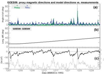
devi-Figure 5.Validating the proxy method of using measurements from
a neighboring satellite.(a)In this 1-month period, deviation angles
between the proxy magnetic field direction and in situ measure-ments (green) along the GOES-09 orbit are plotted as a function of time, compared to angles between T01s model and measurements
(blue).(b)During the period, the relocation of GOES-09 makes its
longitude separation with GOES-8 varying from∼15◦to up to 40◦.
(c)Dst (black) and Kp (gray) indices. Minor and moderate magnetic
activity is observed during the period.
ations in the modeled magnetic field are from both temporal and spatial features, the above equation assumes that the de-viations in two neighboring satellites are homogeneous due to their proximity. Obviously, the validity of this assumption degrades with increasing longitude separation between two satellites.
Derived T01s
A
ngle in b/t (deg)
Date (MMDD in 2004)
1991-080: derived magnetic directions, model directions vs. proxy directions
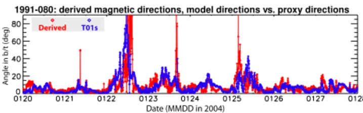
Figure 6. Time series of deviation angles between derived and
proxy magnetic field directions (red) and deviation angles between model and proxy directions (blue). This example covers the same 8-day period in 2004 as in Fig. 2, which includes an intense storm
with the minimum Dst∼ −150 nT on 22 January. The proxy
mag-netic field for LANL-GEO 1991-080 is derived from in situ
mea-surements of NOAA GOES-10 with a∼30◦longitude separation.
field data are available for both. As mentioned, GOES satel-lites generally have a large longitude separation of ∼60◦
, but this separation can be smaller when a GOES satellite is relocated, although observation data during those periods are rarely available. We were fortunate enough to identify a short period with available data in 1995 when GOES-09 was moved from longitude 270 to 244◦
. This movement makes the longitude separation between GOES-09 and GOES-08 increase from initially ∼15 to ∼40◦. Therefore, after ap-plying the above equation to approximating GOES-09 mag-netic field using GOES-08 measurements, proxy magmag-netic field directions are validated by GOES-09 measurements, as the green curve in Fig. 5a. For comparison, deviation an-gles between GOES-09 measurements and T01s model are also plotted. It is clear that the proxy outperforms the T01s model significantly when the longitude separation between satellites is<∼30◦
, and both perform similarly even when the separation goes beyond∼40◦
by the end of the period. Therefore, since the longitude separation between GOES-10 and 1991-080 is ∼30◦in 2004, this proxy method can add the pointP to the plot by using GOES-10 to derive proxy for
1991-080.
First, locating pointPrequires knowing the lengths ofDP
andMP. Therefore, the proxy field directions are compared to derived and model field directions for 1991-080, and Fig. 6 presents a short interval as an example. A statistical study gives out an averagedDP value of 5.34 and anMP value of 4.11. Thus, we are able to plot the pointP for proxy
direc-tions in Fig. 7b.
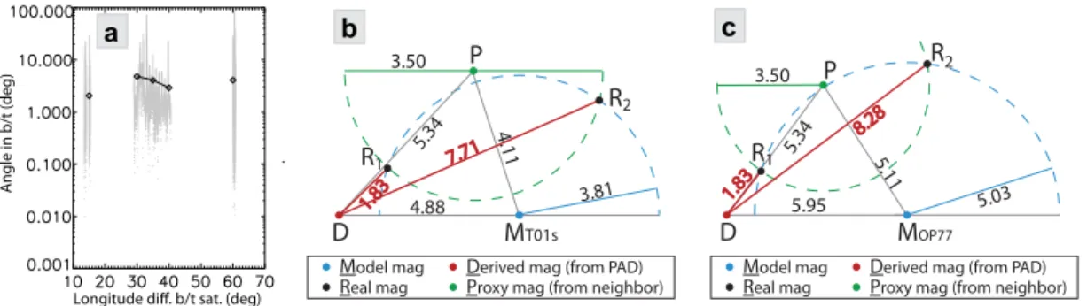
Then we need to derive the value of P R for the cir-cle radius. Besides the above validation using the pair of GOES-08, -09 in December 1995, we also use data from two other periods: GOES-08, -09 between 20 November and 1 December 1997, and GOES-10, -12 between 1 March and 1 April 2004, both with a longitude separation of 60◦
. Devi-ation angles between derived and proxy field directions for all three periods are plotted against longitude separation in Fig. 7a, overplotted by averaged angle values ranging from ∼2 to 5. Here we use the average value of 3.50 for the
seg-ment lengthP R. As in Fig. 7b, the circle⊙P with aP R
radius of 3.50 intersects with the circle⊙MT01s(with a
ra-dius of 3.81): the intersection pointR1has a distance of 1.83
fromD, and the intersection pointR2has a distance of 7.71.
So now the question is which point –R1orR2or both – is
real.
To answer the question, we replace the T01s model with the OP77 model and repeat all of the steps above. As in Fig. 7c, we have different values ofDM,MP, andMRdue to the different model but the same values ofDP andP R, and again there are two intersectionRpoints. However,DR1
in both panels b and c has the same values but theDR2 val-ues are different, which serves as the first piece of evidence thatR1should be the realRpoint since we do expect theDR
values to be independent of empirical magnetic field models. 3.3 Locating pointRfrom grouping of points
Inspired by the proxy pointP added in Fig. 7, we
specu-late that an alternative way of using two empirical models should also be able to add an extra point. As in Fig. 8a, after using the T01s model to place the baselineDMT01s and drawing the circle⊙MT01s, an extra pointMop77from
the model OP77 can be located from the segment lengths ofDMop77andMop77MT01susing 1991-080 data. Then the second circle⊙MOP77is drawn with the radius ofMOP77R
determined from GOES-10 data. Again the two circles have two intersection points: theR1point with a distance of 1.10
from pointD, andR2with a distance of 8.73. To
differenti-ateR1andR2, we introduced the second extra pointMT89
using the model T89, whose position is located from the seg-ment lengths of DMT89 and MT89MT01s using 1991-080 data (panel b). And the third circle⊙MT89, with a radius of
3.81 from GOES-10 data, intersects with the circles⊙MT01s
(⊙MOP77)at pointsR1aandR2a(R1bandR2b). In the ideal
case,R1,R1a, andR1b should overlap (the same is true for R2,R2a, andR2b), though it is natural to see that they do
not do so exactly since statistically averaged values are used here. However, pointsR1,R1a, andR1b in panel b are
in-deed tightly clustered but not pointsR2,R2a, andR2b, which
serves as the second piece of evidence thatR1points should
be very close the real position of theRpoint, instead of the
widely spreading pointsR2,R2a, andR2b.
Angle in b/t (deg)
Longitude dif. b/t sat. (deg) Proxy mag (from neighbor) Model mag Derived mag (from PAD) Real mag
b a
R1
P
R2
3.50
MT01s
D
4.88 3.81
5.34 4.11
7.71
1.83
MOP77
D
5.95 5.03
5.34
P
5.11
8.28
1.83 3.50
R1
R2
c
Proxy mag (from neighbor) Model mag Derived mag (from PAD) Real mag
Figure 7. Determining the position of R point(s) using proxy magnetic field. (a)Deviation angles between proxy and measured field
directions, in three selected periods, are plotted against the longitude separations between each pair of GOES satellites. Overplotted data
symbols are averaged angles for binned longitude separations.(b)The introduction of the pointP and theP Rcircle generateR1andR2
intersection points when T01s model is used.(c)The introduction of the pointPand its circle generate another pair ofR1andR2intersection
points when OP77 model is used.
MT01s D 4.88
3.57
5.95 MOP77
3.81
R1
R2
5.03
8.73
1.10 R1a
D M1a R1b
M1b M2a
M2b
c
a R
2b
R2a
DRm1 DRm2
Model mag Derived mag (from PAD) Real mag
MT01s D 4.88
3.57
5.95 MOP77
3.81
R1 R2
5.03
8.73 1.10
b
MT89
3.81 R1aR1b
R2a R2b
Figure 8.Determining the position ofRpoint(s) using multiple empirical models.(a)A circle is drawn around each of the pointsMT01s
andMOP77from the two models, and the intersections give two candidate pointsR1andR2.(b)The introduction of another pointMT89
(from the T89 model) and its circle generateR1aandR1bpoints very close to theR1, as well asR2aandR2bpoints spreading away from
R2.(c)R1andR2points are determined for different magnetic activity categories. Since theDRm1andDRm2basically stay constant with
magnetic activity, the grouping ofR1points should be much tighter than that ofR2points.
How theDRvalue varies with magnetic activities can be learned in a similar way, by taking advantage of the fact that length difference between theDM andRMlength stays al-most unchanged with magnetic activity levels as discussed in the beginning of this section. A qualitative instead of quan-titative method is employed in this step, which should guar-antee that our conclusion is reliable. As in Fig. 8c, we draw a diagram using two magnetic field models (1 and 2) for two different activity categories (a and b). As just mentioned, since the distances from D to the circles around M1a and M1balong theDM1aline have the constant value ofDRm1,
and the circles around M2a andM2b (not drawn here) will
both be at a tangent with the small circleDwith a radius of
DRm2, we can see that the intersection pointsR1a(between
⊙M1aand⊙M2a)andR1b(between⊙M1band⊙M2b)stay
very close to each other while R2a andR2b are well
sepa-rated. Therefore, because we already know that theR1group
is close to the realRpoint, we conclude thatDRvalues are
not sensitive to the magnetic activity levels. This supports our hypothesis that the observed increasingDMvalues with elevated activity levels in Figure 3 should be mainly due to the degrading performance of empirical models, as discussed in the beginning of this section.
4 Discussion and applications
One possible major error for this study comes from the sta-tistical approach itself, that is, how representative the aver-age points are in the construction plots, such as Figs. 4, 7, and 8. For an individual case study, each point in those fig-ures is definite and thus the triangulation method is valid. However, for two given distributions, the representativeness of the calculated mean deviation points may be questionable. Indeed, considering the variations in each distribution, the above method is only valid when the two distributions are rel-atively homogeneous, which again cannot be directly tested due to the lack of simultaneous derived and measured mag-netic field data. Nevertheless, one indirect test can give us some indications and thus confidence for the representative-ness of averages: in Fig. 8b, the distance betweenMT89 and MOP77can be measured from the plot to be 5.49. Compared
to the calculated value of 4.66, this indicates a∼18 % error that should be acceptable.
Figure 9.Electron PADs – based upon the derived magnetic field directions – observed by LANL-01A SOPA during a geomagnetic storm
period (7 days).(a)Pitch-angle-resolved fluxes for low-energy (131 keV) electrons evolve with time.(b)Pitch-angle-resolved fluxes for
high-energy (1.2 MeV) electrons evolve with time.(c)Dst (black) and Auroral Electrojet (AE) (gray) indices for the period. The time bin
size for each PAD is 4 min. LANL-01A reaches the noon local time position at∼23:00 UT each day during this period.
bin size can be∼11◦so that the assigned pitch angles can have errors as large as∼5.5◦. The second error source may be at times when particle distributions are close to isotropic. This can be significant for low-energy plasma particularly during substorm injections but should be alleviated for en-ergetic radiation belt electrons (typically with several hun-dred keV to >1 MeV energies like the SOPA E5 and ESP E1 channels selected for this work). For example, according to a recent pitch angle distribution (PAD) statistical study, PADs for∼150 keV electrons atL∼6 are statistically very close to isotropic during substorms as shown in Fig. S2b, panels A2 and B2, in the Supplement of Chen et al. (2014), while PADs for∼1.5 MeV electrons at the sameLare statis-tically highly anisotropic as in Fig. S2b, panels A2 and B2. Another possible error source is the intrinsic asymmetry in PAD due to either the statistical fluctuations in counts regis-tered by instruments or some process that breaks down the particles’ bounce movement. The former occurs when MeV electron fluxes drop significantly during storm main phases; the latter may also be possible for electrons close to the loss cone but can be ignored for stably trapped populations that make up the LANL GEO observations. All these could con-tribute to the small but existing errors we found here.
A direct application of the derived magnetic field direc-tion is to sort LANL GEO particle direcdirec-tional measurements into PADs, as one such example shown in Fig. 9. During this double-dip storm period, substorm electron PADs in panel a vary differently from those of energetic electrons in panel b. For instance, substorm electron PADs are mainly pancake-shaped or close to isotropic during injections (e.g. at ∼40 and 125 h), while MeV electrons show intriguing sustained butterfly PADs in the early phase of radiation belt enhance-ments (e.g., throughout the day 19 March). This difference
suggests that the two populations should have experienced different physical processes. Therefore, as discussed in the “Introduction” section, LANL GEO measurements have high energy and pitch angle resolutions and are distributed over multiple longitudes at GEO; thus, they are highly valuable for studying radiation belt dynamics, particularly together with simultaneous observations from Van Allen Probes in-side GEO.
Additionally, since the deviation ofBdis small, we may
use the derived directions as real ones to test the performance of empirical models over the long term (1997–2004). Fig-ure 10 presents the distributions in the same format as in Fig. 3. Percentage distributions in panels a and b are similar to those in Fig. 3 except getting slightly flatter, which is con-sistent with the slightly increased mean values in the mag-netic local time (MLT) distributions in panel c. The small spikes at noon are mainly from data before 2000, and how realistic they are will be left to future investigation by ex-amining individual events. This larger data set allows bet-ter coverage with statistical significance extending to higher magnetic activity categories in panels d, e, and f. From low-to moderate-activity categories, dynamic models persistently perform better than the static model; however, an interesting reverse can be seen in distributions for which T01s model has the largest deviation for the very high activity range.
T01s T89 OP77 Average deviation (deg):
6.67 7.03 8.28 A c c u m . pe rc e n t. ( % ) N o rm . pe rc e n t. ( % ) MLT (h) A
ngles in b/t (deg) Angles in b/t (deg) No
. o f d a ta p o in ts
Kp Dst (nT)
LANL-GEO: deri. B vs. models (’97-’04)
(a)
Angles in b/t (deg) Angles in b/t (deg)
A
ngles in b/t (deg)
LANL-GEO: deri. B vs. T01s (’97-’04) LANL-GEO: deri. B vs. models (’97-’04)
T01s T89 OP77 T01s T89 OP77 T01s T89 OP77 (b) (c)
(d) (e) (f)
AE (nT)
A
ngles in b/t (deg)
Figure 10. Results from comparing derived and model magnetic field directions for all available LANL GEO data within 1997–2004.
Panels have the same format as in Fig. 3.(a)Accumulative percentage vs. deviation angles between derived and simulated directions for
three empirical models T01s (black), T89 (green), and OP77 (gray). Mean angle values are also presented.(b)Normalized percentage vs.
deviation angles for T01s model.(c)Mean deviation angles are binned to MLT for the three models, and the vertical gray bars are the error
ranges for T01s model.(d)Deviation angles are binned to Kp ranges using different colors for three models. Again, the vertical bars are error
bars for T01s model. The gray dotted line plots data sample numbers (read by the vertical axis in right).(e)Deviation angles are binned to
Dst.(f)Deviation angles are binned to the Auroral Electrojet Index (AE).
A n n u a l av e . an g le di ff . ( d e g ) Solar max Solar min (a) (b) Year A n n u a l av e . an g le di ff . ( d e g )
Dependence on solar cycle Dependence on satellites’ L-shell
Lm (T01s)
Y= -30.6 + 5.3*X R = 0.41
Figure 11.Model performance of T01s depends on solar cycle and
satellite positions.(a)Annual average angles are plotted as a
func-tion of years for each LANL GEO satellite.(b)Average angles are
plotted as a function ofLm(McIlwainLshell) for each LANL GEO
satellite. Data points are fitted by the gray straight line, whose equa-tion is given on the top of the panel, with a Pearson’s correlaequa-tion coefficient value of 0.41.
(McIlwainLshell) calculated from T01s model, we do see a general trend of increasing deviation values with increasing Lm by linearly fitting those data points. Indeed, the calcu-lated Pearson’s correlation coefficient has a nontrivial value of 0.41. All these suggest that the model T01s performance degrades with increasing L shells (or, latitudes), which is consistent with our general impression of empirical models.
Finally, as mentioned in Sect. 2, we only chose three repre-sentative empirical magnetic field models without including the more recent sophisticated TS05 model. Although previ-ous studies have demonstrated that T01s performs better than many other models (Chen et al., 2005; McCollough et al., 2008), no comprehensive study has been conducted to com-pare between T01s and TS05. Therefore, we cannot simply extend our conclusion to the TS05 model, although there are some clues suggesting comparable performances of T01s and TS05 at GEO: when statistically comparing to observations dominated by GEO data, TS05 has correlation coefficients of (0.92, 0.83, and 0.92) for magnetic field (x,y,z) compo-nents, while T01s has values of (0.91, 0.82, and 0.90) (Tsy-ganenko and Sitnov, 2005). We decide to leave the inclusion of the TS05 model to the future.
5 Summary
sophisticated dynamic Tsyganenko 2001 storm model), we show that the errors in both derived and modeled directions are at least comparable. Second, using a newly developed proxy method as well as comparing results from multiple em-pirical models, we provide for the first time evidence show-ing that derived magnetic field directions should statistically outperform – with a ratio factor of>∼2 between magnetic field deviation angles – the three selected empirical mod-els (including T01s) in matching the real magnetic direc-tions. Additionally, our results suggest that errors in derived magnetic directions are not so much dependent on magneto-spheric activities as the empirical field models. At last, after showing electron PADs observed by LANL GEO satellites, we further use the derived magnetic field directions for test-ing the performance of empirical field models, with results showing dependence on solar cycles as well as GEO satellite positions. This study for the first time demonstrates the va-lidity and the value of using the symmetric nature of particle spin-resolved distributions for deriving local magnetic field directions.
6 Data availability
50 55 60 65 70 75 80 85 90 95 100 105 110
143 144 145 146 147 148 149 150 151 152
Th
e
ta
(d
e
g)
MPA ESP E1+SOPA E5
-30 -25 -20 -15 -10 -5 0 5 10
143 144 145 146 147 148 149 150 151 152
Phi
(d
e
gree
s
)
Day of year 2005
MPA ESP E1+SOPA E5
(a)
(b)
(c)
Date (MMDD in 2005)
Magnetic field directions: MPA-derived vs. SOPA/ESP-derived
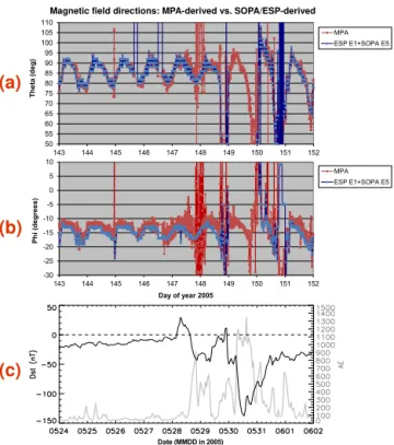
Figure A1. Magnetic field directions derived from MPA aboard
LANL-01A compared to those from SOPA and ESP during a 9-day
period.(a)The time series of magnetic field directions’ polar angle
theta (θ) derived from MPA (red) are compared to those from SOPA
and ESP (blue). LANL-01A crosses midnight at∼23:00 UT each
day in 2005.(b)Time series of field directions’ azimuthal angle Phi
(φ).(c)Dst (black) and Auroral Electrojet (AE) (gray) indices for
the period. A double-dip storm occurred during the period with the
minimum Dst∼ −135 nT reached on 30 May (DOY 149).
Appendix A: Inferring magnetic field directions from LANL GEO SOPA and ESP measurements
The algorithm applied to the SOPA and ESP data first bins each of the three SOPA telescopes and the lone ESP tele-scope into spin phase using accumulations over a 4 min win-dow to flesh out the distribution as a function of spin phase. The count from each accumulation bin is either placed into one of 32 spin-phase bins for SOPA data or into one of 180 spin-phase bins for ESP data. Next, the spin-phase angle,
φ, is found, about which the particle distribution measured by the ESP E1 (0.7–1.8 MeV) channel is most symmetric. This angle points parallel or antiparallel to the projection of the background magnetic field into the plane perpendicular to the spin axis, or, for certain particle distributions, points 90◦
perpendicular to the magnetic field. These ambiguities are cleared up in the second stage of the analysis, wherein every angle,θ, measured from the spin axis, is tested in 2◦
increments as a potential field line direction when combined withφ. The pair (φ,θ )specifies a tested magnetic field di-rection, and the spin-resolved SOPA E5 (225–315 keV)
elec-tron channel counts are binned into pitch angles under the assumption that this pair is the correct one. A smooth poly-nomial function is fitted to the pitch angle binned counts, and the root mean squared error (RMSE) of the fit is calculated. The pair (φ,θ )that produces the lowest RMSE is chosen as the field direction. Because the three telescopes for SOPA may not be perfectly calibrated to one another, multiplicative constants for T1and T3are found that map the pitch angle binned counts for T1 and T3so that they best match those from T2. This “calibration” of T1and T3is done separately for each 4 min time bin, each energy channel, and each hy-pothesized magnetic field direction (φ,θ ). SOPA Channel E5 was chosen to estimate the magnetic field direction because it had the best combination of anisotropy and count rate over the broadest range of conditions, but a better algorithm could be devised that analyzes all energy channels simultaneously, as in Thomsen et al. (1996), or selects the best energy at any given time.
Acknowledgements. This work was supported by the Los Alamos National Laboratory internal funding, the NASA Heliophysics Guest Investigators program (14-GIVABR14_2-0028), and the LANL Center of Space and Earth Science (CSES) program (special large project 2015-007). We want to acknowledge the PIs, instru-ment teams, and data support teams of LANL GEO SOPA and ESP, NOAA GOES magnetometer, as well as the data hosts CDAWeb and SSCWeb. We are grateful for the use of IRBEM-LIB codes for cal-culating magnetic coordinates. We also want to thank the referees for providing constructive and helpful comments that are incorpo-rated into this paper.
The topical editor, G. Balasis, thanks three anonymous referees for help in evaluating this paper.
References
Baker, D. N., Belian, R. D., Higbie, P. R., and Klebesadel, R. W.: Deep dielectric charging effects due to high-energy electrons in Earth’s outer magnetosphere, J. Electrostat., 20, 3–19, 1987. Belian, R., Gisler, G., Cayton, T., and Christensen, R.: High-Z
ener-getic particles at geosynchronous orbit during the great solar pro-ton event series of October 1989, J. Geophys. Res., 97, 16897– 16906, 1992.
Belian, R. D., Cayton, T. E., Christensen, R. A., Ingraham, J. C., Meier, M. M., and Reeves, G. D.: Relativistic electrons in the outer zone: An 11 year cycle; Their relation to the solar wind, in: Workshop on the Earth’s Trapped Particle Environment, New York: Am. Inst. Phys. Conf. Proc., 13–18, 1996.
Chen, Y., Friedel, R. H. W., and Reeves, G. D.: Multisatellite determination of the relativistic electron phase space density at geosynchronous orbit: Methodology and results during ge-omagnetically quiet times, J. Geophys. Res., 110, A10210, doi:10.1029/2004JA010895, 2005.
Chen, Y., Reeves, G. D., and Friedel, R. H. W.: The energization of relativistic electrons in the outer Van Allen radiation belt, Nat. Phys., 3, 614–617, doi:10.1038/nphys655, 2007a.
Chen, Y., Friedel, R. H. W., Reeves, G. D., Cayton, T. E., and Chris-tensen, R.: Multisatellite determination of the relativistic electron phase space density at geosynchronous orbit: An integrated in-vestigation during geomagnetic storm times, J. Geophys. Res., 112, A11214, doi:10.1029/2007JA012314, 2007b.
Chen, Y., Friedel, R. H. W., Henderson, M. G., Claudepierre, S. G., Morley, S. K., and Spence, H.: REPAD: An empirical model of pitch angle distributions for energetic electrons in the Earth’s outer radiation belt, J. Geophys. Res., 119, 1693–1708, doi:10.1002/2013JA019431, 2014.
Huang, C.-L., Spence, H. E., Singer, H. J., and Tsyganenko, N. A.: A quantitative assessment of empirical magnetic field models at geosynchronous orbit during magnetic storms, J. Geophys. Res., 113, A04208, doi:10.1029/2007JA012623, 2008.
Li, X., Baker, D. N., Temerin, M., Reeves, G., Friedel, R., and Shen, C.: Energetic electrons, 50 keV to 6 MeV, at geosynchronous or-bit: Their responses to solar wind variations, Adv. Space. Res., 3, S04001, doi:10.1029/2004SW000105, 2005.
McCollough, J. P., Gannon, J. L., Baker, D. N., and Gehmeyr, M.: A statistical comparison of commonly used exter-nal magnetic field models, Adv. Space. Res., 6, S10001, doi:10.1029/2008SW000391, 2008.
Meier, M. M., Belian, R. D., Cayton, T. E., Christensen, R. A., Gar-cia, B., Grace, K. M., Ingraham, J. C., Laros, J. G., and Reeves, G. D.: The Energy Spectrometer for Particles (ESP): Instrument description and orbital performance, in: Workshop on the Earth’s Trapped Particle Environment, New York: Am. Inst. Phys. Conf. Proc., 383, 203–210, 1996.
Meredith, N. P., Johnstone, A. D., Szita, S., Horne, R. B., Ander-son, R. R.: “Pancake” electron distributions in the outer radiation belts, J. Geophys. Res., 104, 12431–12444, 1999.
Olson, W. and Pfitzer, K.: Magnetospheric magnetic field model-ing, Tech. Rep., McDonnell Douglas Astronaut. Co., Huntington Beach, California, 1977.
Reeves, G. D., McAdams, K. L., Friedel, R. H. W., and O’Brien, T. P.: Acceleration and loss of relativistic elec-trons during geomagnetic storms, Geo. Res. Lett., 30, 1529, doi:10.1029/2002GL016513, 2003.
Reeves, G. D., Chen, Y., Cunningham, G. S., Friedel, R. W. H., Hen-derson, M. G., Jordanova, V. K., Koller, J., Morley, S. K., Thom-sen, M. F., and Zaharia, S.: Dynamic Radiation Environment Assimilation Model: DREAM, Adv. Space Res., 10, S03006, doi:10.1029/2011SW000729, 2012.
Singer, H. J., Matheson, L., Grubb, R., Newman, A., and Bouwer, S. D.: Monitoring space weather with the GOES magnetometers, in: GOES-8 and Beyond, edited by: Washwell, E. R., Proc. SPIE, Vol. 2812,299–308, Int. Soc. for Opt. Eng., Bellingham, Wash-inghton, 1996.
Thomsen, M., McComas, D., Reeves, G., and Weiss, L.: An obser-vational test of the Tsyganenko (T89a) model of the magneto-spheric field, J. Geophys. Res., 101, 27187–27198, 1996. Tsyganenko, N. A.: A magnetospheric magnetic field model with a
wrapped tail current sheet, Planet. Space Sci., 37, 5–20, 1989. Tsyganenko, N. A. and Sitnov, M. I.: Modeling the dynamics of
the inner magnetosphere during strong geomagnetic storms, J. Geophys. Res., 110, A03208, doi:10.1029/2004JA010798, 2005. Tsyganenko, N. A., Singer, H., and Kasper, J.: Storm time distortion of the inner magnetosphere: How severe can it get?, J. Geophys. Res., 108, 1209, doi:10.1029/2002JA009808, 2003.