Observed and predicted characteristics of equatorial F1 layer during solar minimum

(1)

www.ann-geophys.net/32/571/2014/ doi:10.5194/angeo-32-571-2014

Observed and predicted characteristics of equatorial F1 layer

during solar minimum

C.-C. Lee

General Education Center, Chien Hsin University of Science and Technology, No.229, Jianxing Rd., Zhongli City, Taoyuan County 320, Taiwan

Correspondence to:C.-C. Lee ([email protected])

Received: 25 November 2013 – Revised: 8 April 2014 – Accepted: 15 April 2014 – Published: 28 May 2014

Abstract. This study aims to assess the predictability of IRI-2012 on the equatorial F1 layer during solar minimum. The observed characteristics of F1 layer by the Jicamarca digisonde are compared with the model outputs. The results show that the time range for F1-layer appearance of observa-tion is longer than that of IRI-2012, by at least 1 h in the early morning and later afternoon. In IRI-2012, there are three options for the occurrence probability of F1 layer: IRI-95, Scotto-97 no L, and Scotto-97 with L options. The first option predicts the probability well, but the last two underes-timate the probability. The peak density of F1 layer (NmF1) of observation is very close to that of IRI-2012. For the F1 peak height (hmF1), the modeled values are smaller than the observed ones. The observed seasonal variation of hmF1 is not found in the modeled results. Nevertheless, the observed diurnal variation of hmF1 is similar to the modeled results with the B0 choices of Bil-2000 and ABT-2009. Regarding the shape parameter, the values of D1 (the shape parameter of F1 layer in observation) are much greater than the values of C1 (the shape parameter of F1 layer in IRI-2012). The D1 values are 3–6 times the C1 values. The diurnal variation of D1 is similar to that of C1, but the seasonal variation of D1 is not.

Keywords. Ionosphere (equatorial ionosphere; modeling and forecasting)

1 Introduction

In 1969, the Committee on Space Research (COSPAR) and the International Union of Radio Science (URSI) initiated the International Reference Ionosphere (IRI). IRI is an empirical standard model of the ionosphere, based on all worldwide

available data from ground-based and satellite observations (e.g., Bilitza, 1990). Since the late 1960s, IRI has been con-tinuously improved with newer data and better model tech-niques. These processes have resulted in several major mile-stone editions of the model, including the IRI-78 (Rawer et al., 1978), IRI-85 (Bilitza, 1986), IRI-1990 (Bilitza, 1990), IRI-2001 (Bilitza, 2001), and IRI-2007 (Bilitza and Reinisch, 2008). The latest edition of IRI model is the IRI-2012 (http: //iri.gsfc.nasa.gov/).

In order to evaluate the predictability of IRI, the modeled outputs are usually compared with measured ionospheric variables. In the equatorial ionosphere, there were many studies applying ionosonde and digisonde data to validate the F2-layer parameters of IRI model (Adeniyi and Adim-ula, 1995; Adeniyi and Radicella, 1998a, b; Reinisch and Huang, 1998; Adeniyi et al., 2003; Obrou et al., 2003; Abdu et al., 2004; Batista and Abdu, 2004; Lee and Reinisch, 2006, 2012; Lee et al., 2008). The F2-layer parameters are the F2-layer peak electron density (NmF2), its height (hmF2), and the bottom-side profile parameters (B0 and B1). In these previous studies, the comparisons between the ob-served and predicted results were conducted in different lon-gitudinal sectors and in different solar epochs. Unlike the study of F2 layer, however, there is less work on the equato-rial F1 layer than on the equatoequato-rial F2 layer. Adeniyi (1996) might be the only study, which compared the observed F1-layer peak density (NmF1) and height (hmF1) with the IRI modeled outputs at Ibadan, Nigeria (7.4◦_{N, 3.9}◦_{E; dip} lati-tude: 6.3◦_S).

(2)

572 C.-C. Lee: Observed and predicted characteristics of equatorial F1 layer during solar minimum

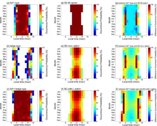
Figure 1.The F1-layer occurrence probabilities for the(a)foF1,(b)ledge, and(c)foF1+ledge types of the Jicamarca digisonde, and for the

(d)IRI-95,(e)SC-no-L, and(f)SC-with-L options of IRI-2012 during January–December 1996. The differences in occurrence probabilities

(g)betweenfoF1 type and IRI-95 option,(h)betweenfoF1 type and SC-no-L option, and(i)betweenfoF1+ledge type and SC-with-L option are presented.

characteristics of IRI is required. The aim of this paper is to investigate how well the IRI-2012 predicts the F1-layer characteristics at Jicamarca, Peru (12◦_{S, 76.9}◦_{W; dip} lati-tude: 1.0◦_{N), during solar minimum. The occurrence} prob-ability, NmF1, hmF1, and profile shape parameter (D1) of F1 layer obtained from the observed ionogram are compared with those modeled by IRI-2012. The data period is between January and December 1996. It is noted that the solar cycle 23 started in May 1996 with the monthly smoothed sunspot number of 8.0.

2 Data

In this study, the ionograms were observed by the Jica-marca digisonde (12◦

S, 76.9◦

W), located near the geomag-netic equator. The recorded ionograms in 1996 provide the hourly data of F1-layer characteristics during solar mini-mum. It is noted that the Jicamarca ionograms were down-loaded from the Digital Ionogram DataBase (DIDBase), and

the ionograms were manually edited with the SAO Explorer software package (http://ulcar.uml.edu/digisonde.html). The occurrence probability is the number of F1-layer events in a certain hour divided by the number of observed ionograms in this hour for a month.NmF1 is calculated from the critical plasma frequency,foF1, of the F1 layer byNmF1 (el m−3₎₌

(3)

Figure 2.The monthly medianNmF1 values for the(a)foF1 and(b)foF1+ledge types of the Jicamarca digisonde, and for(c)SC-no-L and

(d)SC-with-L options of IRI-2012 during January–December 1996. The differences inNmF1(e)betweenfoF1 type and SC-no-L option, and(f)betweenfoF1+ledge type and SC-with-L option are displayed.

fully developed, but a ledge (L-condition) is observed be-low the F2 layer. To eliminate the effects of geomagnetic disturbances, the data only under geomagnetic quiet condi-tions (6Kp≤24) are included in the study. It is noted that the geomagnetic quiet condition is defined as6Kp≤24, where

6Kp is the sum of the eight 3-hourly Kp indices for a day. In addition to the observed data, the values of occurrence probability,NmF1,hmF1, and C1 modeled by the IRI-2012 are applied in this work. C1 is a shape parameter describ-ing the shape of F1-layer profile of IRI-2012 (Bilitza et al., 1990). Because both C1 and D1 are used to describe the shape of F1-layer profile, C1 of IRI-2012 is compared with D1 of observation. The F1-layer occurrence probability of IRI-2012 has three options: (1) IRI-95 (DuCharme et al., 1973), (2) Scotto-97 no L (SC-no-L), and (3) Scotto-97 with L (SC-with-L) (Scotto et al., 1997). It is noted that “L” in the labels of the last two options represents the L-condition (the ledge type of F1 layer) (Scotto et al., 1997). For the IRI-95 option, an F1 layer (foF1 type) is only assumed to exist when the solar zenith angle (χ )is smaller than or equal toχm.χmis

the maximum solar zenith angle, which is calculated from a function of geomagnetic latitude (λ)and 12-month smoothed sunspot number (R12). The detailed definition ofχmcan be found in DuCharme et al. (1973). The occurrence probabil-ity for this option is 0 % (100 %), asχ > χm(χ≤χm). Re-garding the other two options, the occurrence probabilities are calculated from a function of χ, λ, andR12. The defi-nition of the probability function for the no-L and with-L options is described by Scotto et al. (1997). The SC-no-L option gives the occurrence probability of foF1 type,

while the SC-with-L option provides the occurrence proba-bility offoF1+ledge type, which means that bothfoF1 and ledge types are taken together. ForNmF1, only one option is built in the model (DuCharme et al., 1973). RegardinghmF1, the value will be affected by the choice of B0 (Bilitza, 1990). Therefore, all three choices of B0 – (1) Gul-1987 (Gulyaeva, 1987), (2) Bil-2000 (Bilitza et al., 2000), and (3) ABT-2009 (Altadill et al., 2008, 2009) – are applied to modelhmF1. Based on the results of Reinisch and Huang (2000), since IRI-2001, the C1 value has been 2.5 times that of the earlier edition. Furthermore, the observed Ap and F10.7 indices are inputted in the IRI modeling to consider the month-to-month variability. Also, the hourly data of occurrence probability, NmF1, hmF1, and C1 under geomagnetic quiet conditions are used in this study.

3 Results and discussions 3.1 Occurrence probability

Figure 1a–c show that the occurrence probabilities of F1 layer, obtained from the Jicamarca ionograms, for the (a)foF1, (b) ledge, and (c)foF1+ledge types during January– December 1996. For thefoF1 type (Fig. 1a), the F1 layer appears from 08:00 to 16:00 LT. The occurrence probabil-ity does not vary with the seasons. The occurrences are almost 100 % during 10:00–14:00 LT, and exceed 80 % at 09:00 and 15:00 LT. This demonstrates that the F1 layer of foF1 type certainly appears, whenχ is smaller than 35◦

(4)

15:00–17:00 LT. The seasonal variation is also not found in the ledge type. In Fig. 1c, it is found that the appearance be-gins at 07:00 and ends at 17:00 LT, when thefoF1 and ledge types are taken together. The occurrences are almost 100 % between 08:00 and 16:00 LT. This indicates that the F1 layer of foF1+ledge type certainly appears, asχ <65◦

. For the foF1 type, the occurrence probabilities in this study are sim-ilar to the results at low solar activity in Adeniyi (1996) and Adeniyi and Radicella (1997). Adeniyi (1996) and Adeniyi and Radicella (1997) investigated the equatorial F1 layer at Ibadan, Nigeria (7.4◦

N, 3.9◦

E; dip latitude: 6.3◦ S), and Ouagadougou, Burkina Faso (12.4◦

N, 1.8◦

W; dip latitude: 5.9◦

N), respectively. For the ledge type, Adeniyi and Radi-cella (1997) also reported that, at low solar activity, this type of F1 layer generally appears in the early morning and late afternoon. This result reveals that a ledge-like profile occurs just at the bottom of F2 layer, when an F1 layer starts to be formed in the early morning. And, before the layer vanishes, thefoF1-type F1 layer transforms into the ledge type in the late afternoon.

The occurrence probabilities of F1 layer predicted by IRI-2012 are displayed in Fig. 1d–f. The results for the options of IRI-95, SC-no-L, and SC-with-L are presented in Fig. 1d, e, and f, respectively. In Fig. 1d, the occurrence probabil-ities are 100 %. The appearance is during 09:00–15:00 LT for January–March and September–December, and during 10:00–14:00 LT for April–August. For the no-L and SC-with-L options, the occurrence probability will be outputted by IRI-2012, when its value is greater than or equal to 50 %. In Fig. 1e, the time ranges of appearance for the SC-no-L option are the same as those for the IRI-95 option. The occurrence probability has a diurnal variation with a daily maximum value at 12:00 LT. Moreover, the occurrence prob-abilities are larger in the summer and equinoctial months but smaller in the winter months. In Fig. 1f, it is found that the diurnal and seasonal variations for the SC-with-L option are similar to those for the SC-no-L option. Nevertheless, the oc-currence probability and time range of appearance for the with-L option are slightly larger than those for the SC-no-L option.

Figure 1g–i present the differences in occurrence proba-bilities between observation and model. In Fig. 1g, the oc-currence probabilities of IRI-95 option are compared with those of observation (foF1 type). It is found that the IRI-95 prediction is close to the observation during 10:00–14:00 LT. The positive differences exist at 08:00–09:00 LT and 15:00– 16:00 LT, because the time range of appearance is not pre-dicted well by the IRI-95 option. Figure 1h shows the com-parison result between observation (foF1 type) and SC-no-L option, while Fig. 1i displays the comparison result be-tween observation (foF1+ledge type) and SC-with-L option. In Fig. 1h and 1i, it is found that the time ranges of appear-ance of the two options are shorter than those of observa-tion, too. These results suggest that the time range of appear-ance predicted by IRI-2012 should be extended by at least 1 h

Figure 3.The monthly medianhmF1 values for the(a)foF1 and

(b)foF1+ledge types of the Jicamarca digisonde during January– December 1996.

in the early morning and late afternoon. Furthermore, both SC-no-L and SC-with-L options significantly underestimate the occurrence probabilities, except during 11:00–13:00 LT of January–March and September–December. These signif-icant differences are mainly because the seasonal variation in occurrence probabilities does not exist in the Jicamarca observation. These results demonstrate that the SC-no-L and SC-with-L options (Scotto et al., 1997) do not predict the oc-currence probability of F1 layer well.

3.2 Peak density

(5)

Figure 4.The monthly medianhmF1 values for(a)SC-no-L and(b)SC-with-L options, modeled by IRI-2012 with the B0 choice of Gul-1987, during January–December 1996. The differences inhmF1(c)betweenfoF1 type and SC-no-L option, and(d)betweenfoF1+ledge type and SC-with-L option are displayed.

χ. Here, the correlation coefficient between log(NmF1) and log[cos(χ )] for each month is calculated. The correlation co-efficient is estimated to be about 0.98 for all 12 months. This further suggests thatNmF1 can be represented by the relation ofNmF1=a·cosn(χ ). The values ofa andnare derived to be 2.50×1011ele m−3_{and 0.33, respectively. The}_n_{of 0.33}

indicates that the F1 layer is not an idealized Chapman layer, whosenis 0.5 (e.g., Rishbeth and Garriott, 1969). Moreover, according to Rishbeth and Garriott (1969),NmF1 would vary slowly with χ compared to the peak density of idealized Chapman layer, because the linear loss rate decreases with an increasing height. The values ofaandnare close to those in Adeniyi and Radicella (1997), in whicha andnwere found to be 2.75×1011ele m−3_{and 0.34. However, there is no}

sea-sonal variation inNmF1 in Adeniyi (1996) and Adeniyi and Radicella (1997).

Figure 2c–d show the monthly median values of NmF1, provided by IRI-2012, during January–December 1996. Be-cause the NmF1 variation of IRI-95 option is the same as that of SC-no-L option, the results of only SC-no-L (Fig. 2c) and SC-with-L (Fig. 2d) options are presented. For both op-tions, the diurnal and seasonal variations appear in NmF1. And these variations generally follow a solar zenith angle variation. The correlation coefficient between log(NmF1) and

log[cos(χ )] is also calculated and the value is 1. It is expected that coefficient is 1, because IRI-2012 applies the relation of NmF1=a·cosn(χ )to predictNmF1. Moreover, the values of

a andnare derived to be 2.45×1011ele m−3_{and 0.20,}

re-spectively.

In Fig. 2e–f, the differences inNmF1 between observa-tion and IRI-2012 are calculated. The apparent differences in Fig. 2e are located at 08:00–09:00 LT and 15:00–16:00 LT. In Fig. 2f, the apparent differences exist at 07:00–08:00 LT and 16:00–17:00 LT. These differences are primarily caused by the shorter time ranges of appearance of IRI-2012. Except the apparent differences, IRI-2012 provides a good prediction of NmF1, because both observed and modeledNmF1 have the same dependence onχ. Nevertheless, it is necessary to notice thata for IRI-2012 is slightly smaller than for observation, whilenfor IRI-2012 is greater than for observation.

3.3 Peak height

(6)

Figure 5.The monthly medianhmF1 values for(a)SC-no-L and(b)SC-with-L options, modeled by of IRI-2012 with the B0 choice of Bil-2000, during January–December 1996. The differences inhmF1(c)betweenfoF1 type and SC-no-L option, and(d)betweenfoF1+ledge type and SC-with-L option are displayed.

withχ. Conversely, the seasonalhmF1 variation shows that hmF1 is positively correlated withχ, becausehmF1 is higher (lower) whenχis larger (smaller) in the winter (equinoctial) months. These suggest that the relationship between hmF1 andχ can not be used to explain thehmF1 variations. Fur-thermore, these diurnal and seasonal variations would not be caused by the E×B vertical velocity, because the velocity would not affect the ionosphere below 200 km (Radicella and Adeniyi, 1999; Lee, 2012). In Fig. 3b, the seasonal varia-tion offoF1+ledge type is similar to that offoF1 type. How-ever, the diurnalhmF1 variation offoF1+ledge type is par-tially different to that of foF1 type, when the ledge type is included. hmF1 descends from 07:00 to 08:00 LT, and then rises to a maximum height at 12:00 LT. Afterward,hmF1 de-scends again, and then rises from 16:00 to 17:00 LT. Since the ledge-like profile (ledge type) is located just below the F2 layer, the hmF1 values are higher in the early morning and late afternoon.

The monthly median values of hmF1, modeled by IRI-2012, are presented in Figs. 4a–b, 5a–b, and 6a–b. It is noted that thehmF1 variations of only SC-no-L and SC-with-L op-tions are shown in these figures, because thehmF1 variation of IRI-95 option is the same as that of SC-no-L option. The hmF1 variations for the B0 choice of Gul-1987 are displayed

in Fig. 4a–b. In Fig. 4a (SC-no-L option), thehmF1 values are highest and lowest in the winter and summer months, respectively. In the summer and equinoctial months,hmF1 starts to rise at 09:00 LT, and has a maximum at 11:00 LT. Af-terward,hmF1 descends to a minimum at 14:00 LT, and then rises again. For the winter months,hmF1 rises gradually dur-ing daytime. For the other option (Fig. 4b), the diurnal and seasonal variations of SC-with-L option are similar to those of SC-no-L option. Figure 4c–d show the differences inhmF1 between observation and IRI-2012 with B0 choice of Gul-1987. The apparent differences are found at 08:00–09:00 LT and 15:00–16:00 LT in Fig. 4c, and at 07:00–08:00 LT and 16:00–17:00 LT in Fig. 4d, because the time range of ap-pearance for IRI-2012 is shorter than for observation. The significant negative differences are located between March and September. On the other hand, IRI-2012 underestimates hmF1 at 12:00–14:00 LT in November and December.

(7)

Figure 6.The monthly medianhmF1 values for(a)SC-no-L and(b)SC-with-L options, modeled by IRI-2012 with the B0 choice of ABT-2009, during January–December 1996. The differences inhmF1(c)betweenfoF1 type and SC-no-L option, and(d)betweenfoF1+ledge type and SC-with-L option are displayed.

SC-with-L option (Fig. 5b) are similar to those of SC-no-L option (Fig. 5a). For the B0 choice of Bil-2000, the differ-ences in hmF1 between observation and IRI-2012 are dis-played in Fig. 5c–d. In addition to the apparent positive dif-ferences due to the shorter time range, the positive differ-ences exist at 08:00–09:00 and 14:00–16:00 LT in January, February, November, and December. Moreover, it is found that IRI-2012 with B0 choice of Bil-2000 significantly over-estimateshmF1 during February–October.

Figure 6a–b present the hmF1 variations of IRI-2012 with B0 choice of ABT-2009. In Fig. 6a,hmF1 has a diur-nal variation with a daily maximum near noon in January, February, and April–September. In March, and October– December,hmF1 starts to rise at 09:00 LT, and has a max-imum at 11:00 LT. Afterward,hmF1 descends to a minimum at 14:00 LT, and then rises again. There is no noticeable sea-sonal variation inhmF1 for this B0 choice. In Fig. 6c–d, the differences inhmF1 between observation and IRI-2012 with B0 choice of ABT-2009 are shown. It is also found that the apparent positive differences due to the shorter time range exist in the early morning and late afternoon. For this B0 choice, IRI-2012 overestimates hmF1 in all 12 months of 1996.

In addition to the differences inhmF1 described above, the seasonal variation in observedhmF1 (Fig. 4) is not similar to those in the IRI-2012 results for all three choices of B0. Overall, IRI-2012 does not give a good prediction ofhmF1 at Jicamarca during solar minimum. Moreover, among three B0 choices, the B0 choice of Bil-2000 provides a better rep-resentation ofhmF1. This is not consistent with the result of Bilitza and Rawer (1990), in which they proposed that the B0 choice of Gul-1987 produced a more accurate value ofhmF1.

3.4 Shape parameter

(8)

Figure 7.The monthly median D1 values for the(a)foF1 and(b)foF1+ledge types of the Jicamarca digisonde, and the monthly median C1 values for(c)SC-no-L and(d)SC-with-L options of IRI-2012 during January–December 1996. The differences between D1 and C1(c)for foF1 type and SC-no-L option, and(d)forfoF1+ledge type and SC-with-L option are displayed.

Figure 7c–d present the monthly median C1 values of IRI-2012 during January–December 1996. It is noted that the C1 value is applied to calculate the monthly median value, when the corresponding NmF1 is greater than 0. Because the C1 variation of IRI-95 option is the same as that of SC-no-L option, the results of only SC-no-L (Fig. 7c) and SC-with-L (Fig. 7d) options are presented. For both options, the diurnal C1 variation has a daily maximum at 12:00 LT. There is no seasonal variation existing in C1. These variations of C1 are expected, because the C1 values are derived from an Epstein function for a given location and time (Bilitza, 1990).

The differences between D1 and C1 are displayed in Fig. 7e–f. The C1 values are evidently smaller than the D1 values in all 12 months of 1996. The positive differences are greater in the summer and winter months, but they are smaller in the equinoctial months. The difference values greater than 1.5 are found at 12:00 LT in May–August and at 13:00 LT in January–February. And the corresponding ratios of D1 to C1 are greater than 6.0, since the C1 values are 0.28– 0.29. Moreover, in the early morning and late afternoon, the difference values are about 0.4, and the corresponding ratio of D1 to C1 is about 3. These results indicate that the D1 val-ues of observation are 3–6 times the C1 valval-ues of IRI-2012 at Jicamarca during solar minimum.

4 Conclusion and summary

In order to know how well IRI-2012 predicts the character-istics of F1 layer near the geomagnetic equator during so-lar minimum, the observed F1-layer characteristics of the

Jicamarca digisonde are compared with the modeled results. The period of observed and predicted data is between Jan-uary and December 1996. It is noted that this period is under the solar minimum between the solar cycle 22 and 23. The characteristics are the occurrence probability,NmF1,hmF1, and D1 (C1) of F1 layer.

For observation, thefoF1 type of F1 layer appears dur-ing 08:00–16:00 LT, while thefoF1+ledge type exists dur-ing 07:00–17:00 LT. However, the time ranges of appearance are between 09:00 and 15:00 LT for the IRI-95 and SC-no-L options, and between 10:00 and 16:00 LT for the SC-with-L option. There is need to extend the time range of appearance predicted by IRI-2012. During 10:00–14:00 LT, the IRI-95 option predicts the occurrence probability offoF1 type well, but the SC-no-L option underestimates the probability. The SC-with-L option underestimates the occurrence probability offoF1+ledge type during 08:00–16:00 LT. Furthermore, the seasonal variation in occurrence probability is not found in the observed result, but it is found in the modeled results of the SC-no-L and SC-with-L options.

(9)

For thefoF1 type,hmF1 begins to ascend at 08:00 LT, has a maximum height at noon, and then falls. This kind of diurnal variation is qualitatively similar to the diurnal hmF1 varia-tions for the B0 choices of Bil-2000 and ABT-2009, except in March and October–December for ABT-2009. However, for all three B0 choices, IRI-2012 generally overestimates thehmF1 values. For thefoF1+ledge type, the diurnalhmF1 variations of observation are different to those of IRI-2012 for all three B0 choices. For the seasonal variation, the ob-servedhmF1 values are highest and lowest in the winter and equinoctial months, respectively. The seasonal variation of observation is not similar to those of the model. Overall, IRI-2012 does not predict thehmF1 values well.

The diurnal variation of D1 has a daily maximum at noon for thefoF1 andfoF1+ledge types. Although this kind of di-urnal variation can be found in C1 of IRI-2012, the values of C1 are obviously smaller than those of D1. The D1 values are greater in the summer and winter months, but they are smaller in the equinoctial months. However, there is no sea-sonal variation in C1. Moreover, the D1 values are 3–6 times the C1 values.

Acknowledgements. C.-C. Lee was supported by the grant of Na-tional Science Council NSC 2111-M-231-001 and NSC 102-2119-M-231-001. The author would like to thank University of Massachusetts Lowell for access to DIDBase (http://ulcar.uml.edu/ DIDBase/). The author also thank the NASA’s National Space Science Data Center (NSSDC) for providing the IRI-2012 model (http://iri.gsfc.nasa.gov/), and the National Geophysical Data Cen-ter (NGDC) (http://www.ngdc.noaa.gov/) for providing data of Ap, sunspot number, and F10.7 solar flux.

Topical Editor H. Kil thanks S. Tulasi Ram and two anonymous referees for their help in evaluating this paper.

References

Abdu, M. A., Batista, I. S., Reinisch, B. W., and Carrasco, A. J.: Equatorial F-layer heights, evening prereversal electric field, and night E-layer density in the American sector: IRI validation with observation, Adv. Space Res., 34, 1953–1965, 2004.

Adeniyi, J. O.: Equatorial F1 characteristics and the international reference ionosphere model, Radio Sci., 31, 893–897, 1996. Adeniyi, J. O. and Adimula, I. A.: Comparing the F2 layer model of

IRI with observations at Ibadan, Adv. Space Res., 15, 141–144, 1995.

Adeniyi, J. O. and Radicella, S. M.: Electron density and height at F1 region minimum gradient at low solar activity for an equato-rial station, Radio Sci., 32, 1867–1874, 1997.

Adeniyi, J. O. and Radicella, S. M.: Diurnal variation of ionospheric profile parameters B0 and B1 for an equatorial station at low so-lar activity, J. Atmos. Soso-lar-Terr. Phys., 60, 381–385, 1998a. Adeniyi, J. O. and Radicella, S. M.: Variation of bottomside

pro-file parameters B0 and B1 at high solar activity for an equatorial station, J. Atmos. Solar-Terr. Phys., 60, 1123–1127, 1998b.

Adeniyi, J. O., Bilitza, D., Radicella, S. M., and Willoughby, A. A.: Equatorial F2-peak parameters in the IRI model, Adv. Space Res., 31, 507–512, 2003.

Altadill, D., Arrazola, D., Blanch, E., and Buresova, D.: Solar activ-ity variations of ionosonde measurements and modeling results, Adv. Space Res., 42, 610–616, 2008.

Altadill, D., Torta, J. M., and Blanch, E.: Proposal of new models of the bottom-side B0 and B1 parameters for IRI, Adv. Space Res., 43, 1825–1834, 2009.

Batista, I. S. and Abdu, M. A.: Ionospheric variability at Brazilian low and equatorial latitudes: comparison between observations and IRI model, Adv. Space Res., 34, 1894–1900, 2004. Bilitza, D.: International Reference Ionosphere: Recent

develop-ment, Radio Sci., 21, 343–346, 1986.

Bilitza, D. (Ed.): International Reference Ionosphere 1990, NSSDC 90-22, Greenbelt, Maryland, 1990.

Bilitza, D.: International Reference Ionosphere 2000, Radio Sci., 36, 261–275, 2001.

Bilitza, D. and Rawer, K.: New options for IRI electron density in the middle ionosphere, Adv. Space Res., 10, 7–16, 1990. Bilitza, D. and Reinisch, B. W.: International Reference Ionosphere

2007: Improvements and new parameters, Adv. Space Res., 42, 599–609, doi:10.1016/j.asr.2007.07.048, 2008.

Bilitza, D., Radicella, S., Reinisch, B. W., Adeniyi, J., Mosert, M., Zhang, S., and Obrou, O.: New B0 and B1 models for IRI, Adv. Space Res., 25, 89–95, 2000.

DuCharme, E. D., Petrie, L. E., and Eyfrig, R.: A method for predicting the F1 layer critical frequency based on the Zurich smoothed sunspot number, Radio Sci., 10, 837–839, 1973. Gulyaeva, T. L.: Progress in ionospheric informatics based on

elec-tron density profile analysis of ionogram, Adv. Space Res., 7, 39–48, 1987.

Huang, X. and Reinisch, B. W.: Vertical electron content from iono-grams in real time, Radio Sci., 36, 335–342, 2001.

Lee, C. C.: Examination of the absence of noontime bite-out in equatorial total electron content, J. Geophys. Res., 117, A09303, doi:10.1029/2012JA017909, 2012.

Lee, C. C. and Reinisch, B. W.: Quiet-conditionhmF2,NmF2, and B0 variations at Jicamarca and comparison with IRI-2001during solar maximum, J. Atmos. Solar-Terr. Phys., 68, 2138–2146, 2006.

Lee, C. C. and Reinisch, B. W.:Variations in equatorial F2-layer parameters and comparison with IRI-2007 during a deep solar minimum, J. Atmos. Solar-Terr. Phys., 74, 217–223, 2012. Lee, C. C., Reinisch, B. W., Su, S.-Y., and Chen, W. S.:

Quiet-time variations of F2-layer parameters at Jicamarca and compar-ison with IRI-2001 during solar minimum, J. Atmos. Solar-Terr. Phys., 78, 184–192, 2008.

Obrou, O. K., Bilitza, D., Adeniyi, J. O., and Radicella, S. M.: Equa-torial F2 layer peak height and correlation with vertical ion drift and M(3000)F2, Adv. Space Res., 31, 513–520, 2003.

Piggott, W. R. and Rawer, K.: U.R.S.I. Handbook of Ionogram In-terpretation and Reduction, Rep. UAG-23A, World Data Center A for Solar Terr. Phys., Boulder, Colorado, 1972.

Radicella, S. M. and Adeniyi, J. O.: Equaotrial ionospheric electron density below the F2 peak, Radio Sci., 24, 1153–1163, 1999. Rawer, K., Bilitza, D., and Ramakrishnan, S.: International

(10)

Reinisch, B. W.: Modern Ionosondes, in: Modern Radio Science, edited by: Kohl, H., Ruester, R., and Schlegel, K., European Geo-physical Society, Katlenburg-Lindau, Germany, 440–458, 1996. Reinisch, B. W. and Huang, X.: Finding better B0 and B1

param-eters for the IRI F2 profile function, Adv. Space Res., 22, 741– 747, 1998.

Reinisch, B. W. and Huang, X.: Redefining the IRI F1 layer profile, Adv. Space Res., 25, 81–88, 2000.

Rishbeth, H. and Garriott, O. K.: Introduction of ionospheric physics, Academic Press, New York and London, 1969. Scotto, C., Mosert de Gonzáles, M., Radicella, S. M., and Zolesi, B.: