A Work Project, presented as part of the requirements for the Award of a Masters Degree in Economics from the NOVA−School of Business and Economics.
An RBC Model with a rich fiscal sector
Sara Cristina Cantarino Valente de Almeida Msc Student No. 512
A Project carried out in the under the supervision of: Professor João Valle e Azevedo
And also with the collaboration of: Sara Riscado (European University Institute)
An RBC Model with a rich fiscal sector*
Abstract
Contributing to the general understanding of fiscal policy effectiveness, this study consists in the reformulation and estimation of the DSGE model developed in Azevedo and Ercolani (2012), to measure the potential relations between the private sector and the consumption and investment components of government expenditures. The estimation results show that public consumption and capital have both a substitutability effect on private factors. For the study of the dynamic effects, the model is augmented with strict fiscal rules, whose imposition creates a "crowding-out" effect of the simulated fiscal policy shocks on government consumption and investment.
Keywords: Public Spending Externalities, Public Investment Externalities, Fiscal Policy, Bayesian Estimation.
1
Introduction
The large-scale fiscal stimulus packages recently applied to overcome the worldwide 2008 finan-cial crisis triggered a general concern with fiscal policy effectiveness.
Focusing on the investigation of the several channels through which government spending and investment can affect the private sector, this study contributes to the vivid discussion by revisiting the concept ofpublic externalities. Considering the existence of a substitution or complementarity rela-tionship between public purchases and private factors, government spending and investment decisions can have collateral effects on the household’s marginal utility of consumption and the production function of final goods. In this context, the core of this work lies in qualifying the nature of such relationships and observe how they influence the impact of fiscal policy.
For a wide scope of empirical literature on this subject the Ricardian equivalence holds and thus, whether the government funds public expenditures through collecting taxes or issuing debt is irrelevant from the household’s point of view. Growing apart from such framework, in the present model the
setting for income taxes and lump-sum transfers from the government allow to observe the costs of debt financing. How such alternative fiscal regime will coexist with the externalities channels in the model economy is yet another key question this work tries to address.
We follow closely the model proposed in Azevedo and Ercolani (2012) to evaluate the nature of the relationship between private and public consumption and investment. The model developed by these authors will help us to understand the research question because it allows government consumption to directly affect the marginal utility of consumption, through a Constant Elasticity of Substitution (CES) consumption aggregator, and public capital to shift the productivity of private factors. We then propose an extension of the model at two distinct levels. In the light of our main objectives, instead of considering public capital productivity1, a CES capital aggregator is added to production function of final goods. Furthermore, following Traum and Yang (2010), two stabilizers of public debt, in the form of income taxes and lump-sum transfers, are imposed to the fiscal policy sector.
Representing the externalities created by public consumption and capital on the private sector, the CES aggregators combine the two types of productive inputs, allowing to observe relationship between both. Moreover, the new fiscal rules enrich the analysis by changing the transmission mechanism of fiscal shocks with fiscal variables responding to the level of the public debt.
Overall, our main interest rises from the fact that despite the extensive theoretical debate, few are the ones who effectively quantify these relationships and observe their role in a model economy with strict fiscal rules and a general production function. To answer our first purpose we estimate the model through Bayesian methods, without fiscal rules. With the results obtained, we report several impulse response functions and two dynamic multipliers related to government consumption an investment shocks, with and without the augmentations described.
Using U.S. data from 1969 to 2008, the estimation results support a substitutability effect between public and private consumption and, to a lesser extent, between public and private capital. Although opposite to the evidence found in Coenen, Straub and Trabandt (2012) for an open economy, both studies reflect the possibility of public and private capital having a weaker relationship than consump-1Simultaneously with strong evidence of substitutability between public and private consumption, the results
tion factors. When looking at the output dynamic multipliers, the value measured from the model with the substitution effects decreases the impact of a public consumption shock from 0.95 to 0.07, whereas with a shock in government investment the value of the output multiplier goes from 1.09 to 0.90, when the substitution effect of public capital is considered. In turn, the imposition of the fiscal rules implies that both shocks have a significant negative effect on economy, due to the distortionary properties of income taxation.
The remaining of the paper is organized as follows. Section 2 makes a brief review of literature on the topic of interest. Section 3 describes the theoretical model of analysis, while section 4 presents the quantitative analysis. Model dynamics are explained in section 5 and section 6 concludes, presenting conclusions and final remarks.
2
Literature Review
The potential of expansionary policy to foster aggregate economic variables as output, consump-tion or employment is an issue widely present in economic literature. Addressing this quesconsump-tion, this paper contributes to two main fields of fiscal policy analysis. First, it explores the existence of cause-effect relationships between either public and private capital or consumption and, secondly, observes the implications of assuming Non-Ricardian Households, through the imposition of strong fiscal rules. Empirical results on the relationship between public and private consumption hold evidence on both substitutability and complementarity hypothesis. A great set of earlier studies departs from a par-tial equilibrium model, using Euler equations to estimate the value for the elasticity of substitution. For example, Karras (1994) addresses different components of consumption, arriving to a general evidence of complementarity between public and private consumption. In contrast, Graham (1993) performs an extension to the model in Aschauer (1985), showing a crowding out effect of public consumption on the private sector, under the assumption of permanent income. Diverging from these studies, our analysis estimates the elasticity of substitution of both factors within a general equilibrium model, like Bouakez and Rebei (2007). The authors use the maximum likelihood estimation method, finding that a government spending shock leads to a persistent increase in the level of private consumption.
pe-riods of the U.S. history, the analysis finds a substitutability effect between public and private capital, as the national rate of capital accumulation rises with an increase in public investment. However, nar-rowing the study, he also observes that public infrastructure capital fosters the productivity of private capital stocks, thus raising private investment. In fact, both effects seem to have an important role in economy, although the thesis of complementarity is slightly preferred among academics. Particularly, some important contributors to this literature include studies on developing countries like Greene and Villanueva (1991) or Blejer and Khan (1984).
Leaning now onto the last focus of our study, under Ricardian equivalence dynamics of fiscal financing assume a passive role (see Leeper (1991)). In these cases, for market clearing purposes, government debt is omitted from the analysis through the adjustment of lump-sump taxes. As an alternative to such absence of public debt issuing theory, the fiscal section of the model economy in the present study is grounded on the work of Traum and Yang (2010). Although with different purposes, the data and assumptions of both studies are quite similar and so will be the fiscal rules. For the Euro Area, Coenen, Straub and Trabandt (2012), while assessing the impact of the European Economics Recovery Plan on the Euro Area GDP, estimates the model with fiscal rules and the aforementioned externality channels. Our approach proposes a slight different study in the sense that they calibrate the share of public capital on the CES aggregator to 90%, whereas we estimate the model unrestricting the share of public capital and calibrating fiscal rules.
3
The Model
The model economy is an extension of the RBC model in Azevedo and Ercolani (2012), with a more general production function and a more complex fiscal block, where income taxes and lump-sum transfers from the government respond to the public debt level.
The Baseline model, which will be later subject to estimation, is achieved after replacing the pri-vate capital factor in the production function,Kj,t, by effective capital, ˜Kt, discarding public capital
productivity,KtG. Furthermore, the augmentation proposed is complete when labor and capital taxes are replaced by an income tax,τi, and the lump-sum transfers from the government,Tt, are
3.1 Households
The model is composed by households that, facing an inter-temporal budget constraint, will choose the level of consumptionCt and work Lt that maximize their lifetime utility. Ct enters the utility
function through a CES aggregator of private and public consumption,Gt, specified as follows:
˜ Ct=
φ(Ct) v−1
v +(1−φ)G
v−1 v t
v v−1
, (1)
whereν∈(0;∞) is the elasticity of substitution betweenCtandGtand the weight of private
consump-tion in the effective consumpconsump-tion aggregator is given byφ.
The households, deriving utility from effective consumption and desutility from working, define their lifetime expected utility as:
E0 ∞ X
t=0
βkeεbt
˜
Ct−hC˜At−1
1−σc
1−σc −χ
1 1+σL(Lt)
1+σL
, (2)
with β∈(0,1) as the subjective discount factor and and χa positive number. εbt represents the preference shock, assumed to follow a first-order autoregressive process with an i.i.d.-normal error term: εbt =ρbεbt−1+ηbt. The aggregate level of effective consumption at time t−1, ˜Ct−A1, introduces an external habit formation degreeh∈(0; 1). The parameter σc denotes the degree of relative risk
aversion andσLis the inverse of the Frisch elasticity of labor supply. The existence of a steady-state growth path is assured by assuming complete separability between consumption and labour, given the neoclassical production function, but requiring settingσcequal to one.
Each household sets the levels of consumption, labor supply, next period’s physical capital stock, Kt+1, level of investment, It, and installed capital stock utilization intensity, ut, subject to taxation
on labor (τw), consumption (τc) and capital (τk), expressed in marginal rates. They participate in a market of state-contingent securities, payingZth+1att+1 if statehrealizes, at the costEt
h 1 1+rt,t+1Z
h
t+1
i , where 1/(1+rt,t+1) is the stochastic discount factor. The budget constraint (expressed in real terms) is
represented as follows:
(1+τc)Ct+It+Et
" 1 1+rt,t+1
Zth+1 #
= (3)
Zth+(1−τw)WtLt+(1−τk)
h
rtkut−a(ut)
i
Kt+DIVt−Tt,
the cost of using capital at intensityut.DIVt are the dividends paid, whileTt are lump-sum transfers
from the government.
As capital enters the decision process with one period discrepancy, the link between capital stock for two consecutive periods is given by:
Kt+1=(1−δk)Kt+It
"
1−S eεIt It
It−1 !#
, (4)
whereδkis the depreciation rate and investment adjustments costs are set in the functionS(.), adopted
from Christiano, Eichenbaum and Evans (2005). S(.)= κ2eεIt It
It−1−e
γ2, whereεI
t is a shock to the
investment cost function that follows a first-order autoregressive process with an i.i.d.-normal error term andγis the steady-state growth rate of productivity.
3.2 Government and Fiscal Policy
For each period, public consumption Gt and investment Itg represent a determined fraction of
output,Gt=ξtgYtandItg=ξ ig
t Yt, whereξtgandξ ig
t follow:
ξtg=exp(εgt +ssg)/(1+exp(εgt +ssg)) ; ξtig=exp(εigt +ssig)/(1+exp(εigt +ssig)).
In turn, real government expenditure and investment shocks,εgt andεigt respectively, are exogenous and stochastic univariate first-order autoregressive processes:
εgt =ρgεgt−1+ηgt (5)
εigt =ρigεiigt−1+ηigt , (6)
whereηgt andηigt are normal i.i.d. and mutually independent with mean zero. ξgt andξigt are defined in order tossgandssig, so that their steady-state levels are fixed :
ssg=log(ξg,ss/(1−ξg,ss)) ; ssig=log(ξig,ss/(1−ξig,ss)).
Given that in this model public investment is split into defense and non-defense items: Itg,de f =ξtig,de fYt
ξgt,de f =exp(εgt,de f+ssg,de f)/(1+exp(εgt,de f+ssg,de f))
where defense investment is Itg,de f, ssg,de f =log(ξg,de f,ss/(1−ξg,de f,ss)) and ηigt ,de f is a normal i.i.d. defense investment shock with mean zero. Note that, with this specification, defense items are not embedded in public capitalItg.
Since the paths ofξtg, ξtigandξtig,de f are considered exogenous while the paths forGt,ItgorI
g,de f
t
are not, facing a drop on the total factor productivity and the output level, government consumption and investment are expected to fall, without intervention of automatic stabilizers.
Whenever the balanced budget hypothesis holds, the following expression defines the govern-ment’s budget constraint:
τcCt+τwWtLt+τk
h
rktut−a(ut)
i
Kt+Tt=Gt+Itg+I
g,de f
t . (8)
With respect to the extension of the fiscal policy section, following Traum and Yang (2010), the extended model sets income tax,τit, and lump-sum transfers from the government, Tt, to depend on
past levels of public debt, Bt.The equations for both fiscal rules, measured in deviations from the
steady-state (denoted with hats), are:
bτit=ρτbτit−1+(1−ρτ)γτbrbt−4+ετt (9)
b
Tt=ρzTbt−1+(1−ρz)γzbrbt−1+εzt (10)
wherebrbt is the debt-to-output ratio,B[t/Yt, andετt andεzt are, respectively, the exogenous shocks
of income tax and lump-sum transfers, both following an i.i.d. normal distribution.
As a result, the new budget constraints for the government and households are respectively defined as:
τcCt+τit(WtLt+
h
rtkut−a(ut)
i
Kt)+Tt+(1+rtb)Bt−1=Bt+Gt+Itg+I
g,de f
t (11)
and (1+τc)Ct+It+Et
" 1 1+rt,t+1
Zht+1 #
+Bt=Zht +(1−τit)(WtLt+
h
rktut−a(ut)
i
Kt)+DIVt−(1+rtb)Bt−1−Tt,
(12) where rbt represents the interest the government needs to pay relative to the debt owed in the previous period,Bt−1.
3.3 Firms and labor market
Each firm j, under a monopolistic competitive set, produces a single variety of final goodsYj,twith
allocate their consumption equally between all goods. In this framework, we can abandon indexjand consider a representative firm that produces a final goodYt, using effective capital ˜Kt, labor Lt and
the fraction of public capital that does not produce any externality, represented by the defense public investmentItg,de f. From the solution of the profit maximization problem, competitive firms set price levelPj,tas a markupλp,ssto the marginal cost. The production function is then given by2:
Yj,t=max(AtK˜tαL1j,−tα−AtΦ,0), (13)
whereΦis the production fixed cost andAt is a productivity shock. The process for ln(At) has a
unit-root and evolves according to:
ln(At)=γ+ln(At−1)+εat, (14)
whereγis the steady-state growth rate of productivity andεat =ρaεt−a1+ηat , whereηat is an i.i.d.-normal sequence.
The effective capital CES aggregator, ˜Kt adopted from Coenen, Straub and Trabandt (2012) is
adjusted to enter the final goods production function of firms, allowing to measure the elasticity of substitution between public and private investment,vk:
˜ Kt=
"
φk(Kt) vk−1
vk +(1−φk) (KtG) vk−1
vk
# vk vk−1
, (15)
where φk is the share of private capital stock in effective physical capital and KtG denotes the "productivity" of public capital. Relatively to the elasticity of substitution, when vk1 private and
public capital are substitutes, for values lower than 1, as it tends to zero the complementarity effect emerges and ifvk=1 any cause-effect relationship is observed.
The public capital and the productivity of defense capital are assumed to evolve respectively ac-cording to:
KtG+1=(1−δKg)KtG+ξ ig
t , (16)
and
KtG+,1de f=(1−δKg,de f)KtG,de f+ξtig,de f (17)
whereδKgis the depreciation rate.
With respect to the Labor Market, households answer the demand that allows setting the wage rate 2The specification is the same as in the model of Azevedo and Ercolani (2012), but in our modelKG
t enters
the production function through the CES aggregator and since we discard the productivity of public capital
Wi,tthat maximizes their utility, according to labor demand,Lt, and aggregate nominal wage,Wt.The
wage setting definesWi,tas a markupλw,t, over the marginal rate of substitution between consumption
and leisure.λw,tis stochastic and exogenous and follows a first order autoregressive process.
3.4 Remaining Considerations
In a standard Real Business Cycle model, prices have perfect flexibility, automatically adjusting to assure market clearing conditions under perfect competition. In equilibrium, supply will equal demand, for every market. Labour demanded by firms equals differentiated labour services supplied by households, at the aggregate wage rateWt , capital services demanded by firms equals capital
supplied by households and the final goods supply equals demand by households and the government: Yt=Ct+It+a(ut)Kt+Gt+Itg+I
g,de f
t . (18)
3.4.1 The Solution
The process for the solution of the steady-state followed the standard procedure of DSGE models solution. Considering identical agents, the first order conditions associated with the households’ and firms’ problems are derived and combined with market clearing conditions and exogenous processes. The variables subject to generational growthCt,It, Kt,Wt,T axt,Tt,Gt, Itg,I
g,de f
t andBt need to be
stationarized by the level of technologyAt. The same treatment is required for the Lagrange multipliers
associated with the budget constraint and the capital accumulation equation, respectivelyΛt andQt
(Tobin’s q). The conditions which solve the equilibrium for the present model can be found in the Appendix C. For estimation purposes, apart from variablesξgt ,ξigt andξigt ,de f, the model equations are log-linearized around the steady state.
4
Identification, Calibration and Estimation
With U.S. quarterly data from 1969Q1 to 2008Q3, the baseline model is identified and estimated by Bayesian methods, using the statistical software platform DYNARE of Matlab.
From the acknowledgment of unidentification issues on the estimation of DSGE models, our anal-ysis attains the identification sufficient conditions established in Iskrev (2010), leaving the analanal-ysis on the strength of identification for later improvements to the study.
in-formation based approach, but only the former is used in the identification package developed for DYNARE3.
Without an exhaustive description of the concept, consider a parameter spaceΘ⊂Rk, defined as the set of all theoretically admissible values of the deep parameters vectorθ. Given the observed data, it is possible to definemT: [µ′, σ′T]′, a (T−1)ℓ2+ℓ(ℓ+3)/2−dimensional vector that collects the
parameters which determine the first two moments of the data,µ′andσ′T. It follows thatmTis a
func-tion ofθ, assuming that to each admissible value ofθcorresponds a unique value ofτ, the vector of the reduced form parameters. In case the model’s random vector of structural shocks,ut, is Gaussian
and no further assumptions on structural shocks are established, the restrictions onmT have all the
useful information for the estimation ofθ. The parameter is identified if that information is sufficient according to the following theorem:
Theorem 1 Considering mT as a continuously differentiable function of the vector of deep
parametersθ,θ0 is locally identifiable if the Jacobian Matrix J(T)= δmq
δθ′ has full column
rank atθ0, for q≤T.
Whenq=T, this conditions is only sufficient for identification ifutis normally distributed. In addition
is also required that the number of deep parameters does not exceed the dimension ofmt.
Because the distribution of the data depends onθthroughτthe program yet triggers theJacobian4 of the transformation fromθ toτ, J2(T). Pointθ0 is locally identifiable if the rank ofJ2(T)= δθδτ′ is
equal to the dimension ofθ. Note that, in practice, deep parameters are unknown. To overcome this issue the program relies on the prior distributions set by the analyst, assuming the mean values as the deep parameters of the model.
With both rank conditions verified, this section proceeds with the report of the Bayesian estima-tion5 results and calibrated parameters. For estimation purposes, seven observable macroeconomic time-series are considered, mapped from the data through measurement equations in log-differences,
3The information matrix is used for the sensitivity analysis, which we do not address in our study 4Denoted by H in DYNARE.
5Dynare uses a Bayesian MH-MCMC algorithm, performing different iterations chains. The initial
except for consumption and investment, which are specified in levels. Data description and measure-ment equations are described in Appendix D.
Bayesian estimation combines the prior probabilities of the parameters with the likelihood func-tion, which when maximized finds the values of the parameters that more probably generated the data, given the prior values defined. This posterior distribution is obtained as:
p(θ|YT)= L(Y
T|θ)p(θ)
∈L(YT|θ)p(θ)dθ,
the quotient between the likelihoodL(YT|θ) and its marginal value, of sample Y, with T
observa-tions and wherep(θ) is the prior probability of vectorθ.
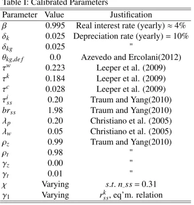
Calibrations and priors imposed to the model’s parameters are shown in Table I. The calibrations enter the estimation process as very strict priors. Generally, these parameters directly affect the steady-state, whereas the ones defining the dynamics of the model are preferably estimated. vk andv are
re-parameterized tovk=evik andv=evb ∈(-∞;+∞), normally distributed with mean−1 and standard
deviation 10. For values less than unity, asvk tends to zero, public and private capital become more
complements. They are considered substitutes for the opposite space and not related ifvk =1. The
share of private capital on the final goods production function,φkis uniformly distributed in the range
[0,1]. Finally, we want to make clear theFiscal Strategymodel is not subject to estimation and thus, tax values are fixed. Nevertheless, on behalf of the remaining empirical evidence we need to specify the calibrations applied to the components of the fiscal rules,ρz,ρt,γz,gammat and the steady state
levels ofbrt andtauit,brss6andtauiss.
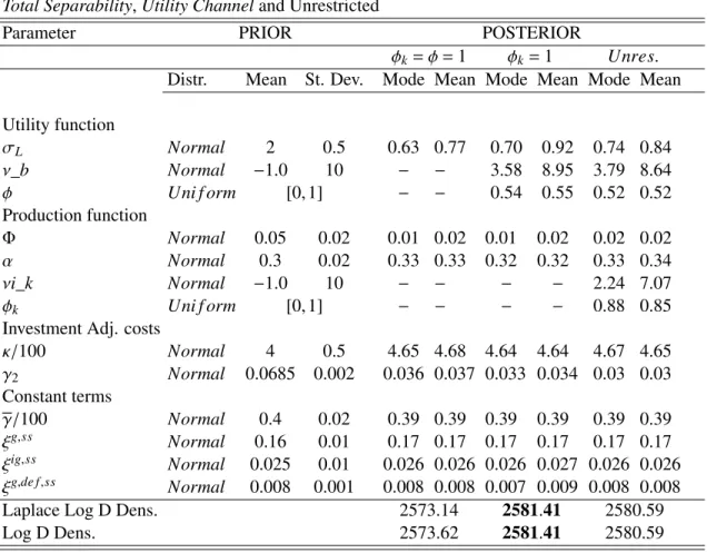
The estimation results for three variations of the baseline model are presented in Table II7. Firstly,
φk andφare both set to unity, showing a model economy where government decisions do not have collateral effects on private inputs. The next stage studies the externality channel on utility, only restrictingφk. Finally, the model is estimated without the imposition of any restrictions.
The highest marginal data is achieved when the externality channel on the production function is closed, with the share of private consumption on utility estimated to be around 52%. As the result obtained in Azevedo and Ercolani (2012), government and private consumption are estimated to be 6The calibrated value in each quarter corresponds to an annual public debt to output ratio around 50% in the
steady state.
Table I: Calibrated Parameters
Parameter Value Justification
β 0.995 Real interest rate (yearly)≈4%
δk 0.025 Depreciation rate (yearly)=10%
δkg 0.025 "
θkg,de f 0.0 Azevedo and Ercolani(2012) τw 0.223 Leeper et al. (2009)
τk 0.184 Leeper et al. (2009)
τc 0.028 Leeper et al. (2009)
τiss 0.20 Traum and Yang(2010)
brss 1.98 Traum and Yang(2010) λp 0.20 Christiano et al. (2005) λw 0.05 Christiano et al. (2005)
ρz 0.99 Traum and Yang(2010)
ρt 0.98 "
γz 0.00 "
γt 0.01 "
χ Varying s.t.n_ss=0.31 γ1 Varying rkss, eq’m. relation
strongly substitutes with a posterior mean forνibof 8.4. Relatively toνik, public and private investment
seem also to be substitutes, but with a weaker relationship. However, the wide confidence interval8of the estimated parameter leaves some reservations regarding the strength of such effect and the accuracy of the estimation9. Besides, the share of private capitalφkis estimated to be 85% with the unrestricted
version, but the accuracy of the model slightly decreases10, which shows preference for the model with φk equal to one. Curiously, the main results are opposite to those found in Coenen, Straub
and Trabandt (2012)11 for an open economy. Still, also in their study, the elasticity of substitution between public and private capital is lower than the one between public and private consumption. In between, Mazraani (2010) finds a substitution effect between private and public consumption and a
8Appendix B.
9Identification issues seem to damage the estimation of this parameter. Further investigations should be done
regarding its specification and contribution to the model.
10Following the work of Smets and Wouters (2003),the overall fit of DSGE models can be measured by its
marginal data density, useful for comparison purposes.
11Please recall that the share of private investment is calibrated by the authors to 90%, the parameterφ
k in
complementarity effect between public and private investment.
Table II Priors and Posteriors of selected parameters 1969Q1-2008Q3 Total Separability,Utility Channeland Unrestricted
Parameter PRIOR POSTERIOR
φk=φ=1 φk=1 Unres.
Distr. Mean St. Dev. Mode Mean Mode Mean Mode Mean Utility function
σL Normal 2 0.5 0.63 0.77 0.70 0.92 0.74 0.84
ν_b Normal −1.0 10 − − 3.58 8.95 3.79 8.64
φ Uni f orm [0,1] − − 0.54 0.55 0.52 0.52
Production function
Φ Normal 0.05 0.02 0.01 0.02 0.01 0.02 0.02 0.02
α Normal 0.3 0.02 0.33 0.33 0.32 0.32 0.33 0.34
νi_k Normal −1.0 10 − − − − 2.24 7.07
φk Uni f orm [0,1] − − − − 0.88 0.85
Investment Adj. costs
κ/100 Normal 4 0.5 4.65 4.68 4.64 4.64 4.67 4.65
γ2 Normal 0.0685 0.002 0.036 0.037 0.033 0.034 0.03 0.03 Constant terms
γ/100 Normal 0.4 0.02 0.39 0.39 0.39 0.39 0.39 0.39
ξg,ss Normal 0.16 0.01 0.17 0.17 0.17 0.17 0.17 0.17
ξig,ss Normal 0.025 0.01 0.026 0.026 0.026 0.027 0.026 0.026
ξg,de f,ss Normal 0.008 0.001 0.008 0.008 0.007 0.009 0.008 0.008
Laplace Log D Dens. 2573.14 2581.41 2580.59
Log D Dens. 2573.62 2581.41 2580.59
5
Model Dynamics
5.1 Dynamic Effects
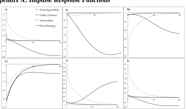
The following section analyses impulse response functions to a shock both in government con-sumption and investment and tries to unveil the main implications behind the imposition of the ex-ternalities channels and fiscal rules. For the simulations we use the posterior mode of the parameters estimated for the unrestricted model12, which generate the lines in the plots displayed from figure 1 to 3.2 in Appendix A. Specifically, figure 1 presents the impulse response functions of a one standard deviation increase in public consumption, figure 2 shows the impact of a shock with the same magni-tude in public investment and in figures 3.1 and 3.2 are alternative versions of the augmented model, 12Although the unrestricted version is not preferred, we opt to use this version since it allows to observe the
again subject to a shock in government spending.
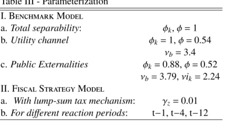
Conditional on specific parameterization (summarized in table III) we define four different ver-sions of the model: theTotal Separability(i) , theUtility Channel(ii), thePublic externality(iii) and theFiscal Strategy (iv). The notation adopted gives intuition for the mechanisms observed in each version. Looking at the figures, the first version, with a dashed grey line, shows the reaction of a model without either substitution effects or fiscal rules (φ=φk=1). Secondly, (ii) considers the public
externality on private consumption and in (iii) we add the substitutability between public and private capital, which are respectively represented by the blue and red dashed lines. Finally, a solid black line is traced for the model with strict fiscal rules13.
Moreover, in the final version –Fiscal Strategy– income tax,τit, depends on the level of public debt one year ago,Bt−4, and supports by itself the burden of public debt (γz=0, as earlier shown in Table
I). We further explore this specification by setting different timings for the government’s reaction and by assuming lump sum transfers to share the funding of public debt withτit.14
Table III - Parameterization
I. BenchmarkModel
a.Total separability: φk,φ=1
b.Utility channel φk=1,φ=0.54
νb=3.4
c.Public Externalities φk=0.88,φ=0.52
νb=3.79,νik=2.24
II. FiscalStrategyModel
a. With lump-sum tax mechanism: γz=0.01
b.For different reaction periods: t−1, t−4, t−12
Regarding the shock in government consumption (figure 1), with theTotal Separability model, output, the interest rate and the level of labor are upward driven, in contrast with private consump-tion, investment and wage level. In turn, when subject to the public externality, private consumption decreases further, because families suffer from the combination of a negative wealth and substitution effect. With respect to the remaining variables, this shock loses impact and the return to the steady is 13Note that although this version was not subject to estimation, this exercise still adopts the posterior mode
estimates of the unrestricted model. We simply adjust thePublic externalityversion with the imposition of the fiscal rules to get theFiscal Strategyframework.
considerably faster. Regarding theFiscal Strategymodel, the decrease of private investment is empha-sized and the decrease in consumption gains persistence. The distortionary tax represents an opposing force to the shock’s expansionary effect and leads output to decrease soon after impact. In addition, an increase on taxes also generates a disincentive to work, reducing the number of hours individuals devote to labor.
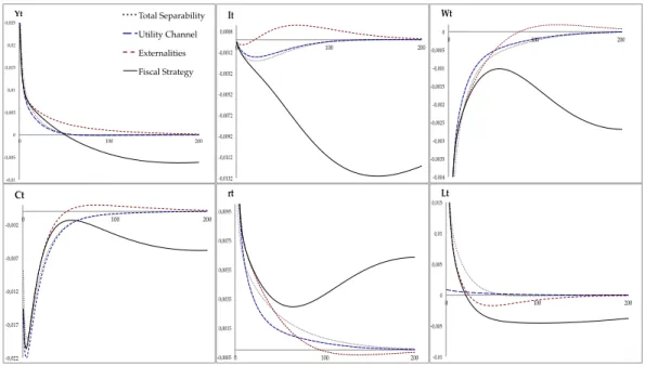
Turning to the effect of a shock in government investment (figure 2), please recall that in the context of the Public Externalities framework public capital competes with private capital. With an increase of the former, the interest rate increases on impact and there is an incentive for private agents to slowdown investment. However, in this case, the negative substitution effect is dominated by a positive wealth effect and investment increases around 6 years after impact. In parallel with the dynamics observed for the previous shock, in the long run, the imposition of fiscal rules represents a deterioration of the living standards at al levels.
Focusing on theFiscal StrategyModel, when government transfers share the funding of the public debt level with tax (figure 3.1), the fiscal policy shock is less damaging. Income taxation,τi, reaches a lower maximum level and the steady state is sooner re-attained. As a result, the output period of adjustment is also shorter and debt reacts to a lesser extent, inclusively dropping with the course of recovery.
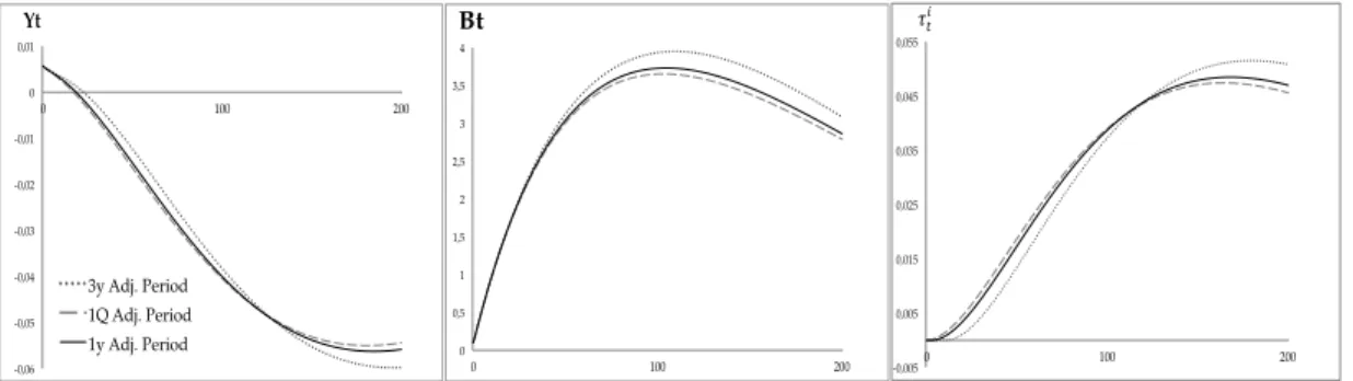
Finally, we assume the government reacts to the debt level by increasing income taxes at the first quarter (t−1) or three years after impact (t−12) (figure 3.2), in alternative to the baseline assumption of one year (t−4). Although the marginal effect is quite low, there is evidence that if government waits longer before increasing taxes the increase will have to be stronger than if the reaction is immediate.
5.2 Government Consumption and Investment Multiplier
Resorting to the formulation in Mountford and Uhlig (2009), to quantify the influence of fiscal policy, dynamic multipliers are computed by discounting the cumulated responses of output facing one standard deviation policy shock. The value for the dynamic multiplier expressed for t quarters after the shock is given by:
ϕt= t
P
k=1
(1+rss)−k∆yk t
P
k=1
where∆yk represents the deviation of output from its steady-state at time k and∆gk represents
the marginal variations of government purchases measured as a fraction of the steady-state output.rss
is the steady-state real interest rate. This multiplier measures the cost of returning to equilibrium, in output terms, inherent to an increase in government consumption/investment.
In tables IV and V are presented the results of the dynamic multipliers of output, in response to the government policy shocks, for different periods.
When any of the externalities mechanism is allowed, the shock of public consumption has a strong effect on output, with the respective impact multiplier reaching a maximum level of 0.95, slightly different from the 1.072 found with the baseline model in Straub and Tchakarov (2007). With public consumption affecting the utility function, the impact on output is much smaller due to the negative wealth and substitution effects on households consumption. Remarkably, the high estimated value of 48%15for the share of public capital on the effective consumption function causes such a low value of the multiplier with the model’s preferred version.
After the the introduction of fiscal rules, the contractionary effect on output is evident in the long-run. Coenen, Straub and Trabandt (2012) uses the same formulation of the multiplier, but finds an effect of 1.02 on impact and 0.84 in the long-run, with consumption and labour taxes adjusting to the public debt value.
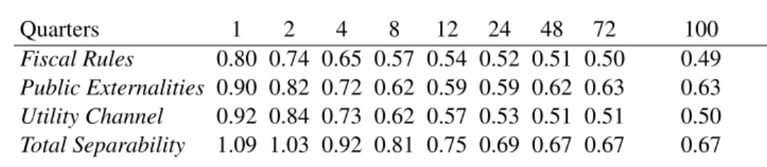
Finally, the output to government investment multiplier for the first quarter decreases from 1.09 to 0.90 when the substitution effect between public an private capital is considered.
All in all, the model dynamics show that a shock in public consumption is generally unproductive, opposite to the effect of an increase in public investment.
Table IV - Dynamic Multipliers,Government Consumption Shockon Output Y
Quarters 1 2 4 8 12 24 48 72 100
Fiscal Rules 0.09 0.09 0.08 0.07 0.06 0.05 0.03 0.01 −0.01 Public Externalities 0.07 0.06 0.06 0.05 0.05 0.04 0.04 0.04 0.04 Utility Channel 0.07 0.06 0.06 0.05 0.05 0.05 0.05 0.04 0.04 Total Separability 0.95 0.90 0.82 0.69 0.65 0.63 0.63 0.62 0.62
15The share of public capital in the CES aggregator is given by (1−φ
Table V - Dynamic Multipliers ofGovernment Investment Shockon Output Y
Quarters 1 2 4 8 12 24 48 72 100
Fiscal Rules 0.80 0.74 0.65 0.57 0.54 0.52 0.51 0.50 0.49 Public Externalities 0.90 0.82 0.72 0.62 0.59 0.59 0.62 0.63 0.63 Utility Channel 0.92 0.84 0.73 0.62 0.57 0.53 0.51 0.51 0.50 Total Separability 1.09 1.03 0.92 0.81 0.75 0.69 0.67 0.67 0.67
6
Concluding Remarks
Two main objectives have driven this study. On one hand, an attempt was made to complement the evidence found in Azevedo and Ercolani (2012) by establishing a more general production function. On the other, in order to observe how the imposed channels behave under a more realistic fiscal policy, the set up economy is extended with more complex fiscal rules.
The empirical evidence shows a substitution relationship between private and public capital. else constant, as public investment increases, firms seem to be discouraged to invest. However, the pres-ence of this externality on the estimated model does not constitute the preferred version and the respec-tive elasticity of substitution is estimated in a wide confidence interval. Given the lack of robustness in these results and the limited set of DSGE models applications to this study, the overall validity of our conclusion is questionable and there is a need for further investigation.
As for public and private consumption, results support the evidence found in Azevedo and Ercolani (2012), showing the model is able to fit the data with a strong substitutability effect even adopting a normal prior distribution centered in complementarity. In this framework, the substitutability effect reduces the capacity of a shock in government spending to foster the output level.
References
[1] Almeida, Vanda. 2009. “Bayesian estimation of a DSGE model for the Portuguese economy." Banco de Portugal: Working papers series 16/2009.
[2] Aschauer, David. 1985. “Fiscal Policy and Aggregate Demand." American Economic Review, American Economic Association, 75(1): 117-27.
[3] Aschauer, David. 1989b. “Is Does Public Capital Crowd Out Private Capital?." Jornal of Mon-etary Economics, 24: 171-188.
[4] Autery, Monica and Costantini, Mauro. 2010. “A panel co-integration approach to estimating substitution elasticities in consumption." Economic Modelling, Elsevier, 273: 782-787. [5] Azevedo, João and Ercolani, Valerio. 2012, “The Effects of Public Spending Externalities."
Bank of Portugal, Economics and Research Department, Working papers 10/2012.
[6] Blanchard, Olivier and Perotti, Roberto. 2002. “An Empirical Characterization Of The Dy-namic Effects Of Changes In Government Spending And Taxes On Output." The Quarterly Journal of Economics, MIT Press, 1174: 1329-1368.
[7] Blejer, Mario and Khan, Mohsin. 1984. “Government policy and private investment in devel-oping countries." IMF StaffPapers, 31(2).
[8] Bouakez, Hafedh and Rebei, Nooman. 2007. “Why does private consumption rise after a gov-ernment spending shock?" Canadian Journal of Economics, Canadian Economics Association, 40(3): 954-979.
[9] Canova, Fabio and Sala, Luca. 2009. “Back to square one: Identification issues in DSGE model." Journal of Monetary Economics, Elsevier, 564: 431-449.
[10] Carvalho, Fabia and Valli, Marcos. 2011. “Fiscal Policy in Brazil through the Lens of an Es-timated DSGE Model". Central Bank of Brazil, Research Department, Working papers series 240.
[11] Christiano, Lawrence J., Eichenbaum, Martin and Evans, Charles L. 2005. “Nominal Rigidities and the Dynamic Effects of a Shock to Monetary Policy." Journal of Political Economy, 113(1). [12] Coenen, Gunter, Straub Roland and Trabandt, Mathias. 2012. “Gauging the effects of fiscal
stimulus packages in the Euro Area." European Central Bank, Working papers 1483.
[13] Coutinho, Rui M. and Gallo, Giampiero M. 1991. Do Public And Private Investment Stand In Each Other’s Way. World Development report background paper, mimeo.Washigton, D.C.:World Bank.
[14] Davig, Troy and Leeper, Eric M. 2011. “Monetary-fiscal policy interactions and fiscal stimu-lus." European Economic Review, Elsevier, 552: 211-227.
[15] Fatás, Antonio and Mihov, Illian. 2001. “Government size and automatic stabilizers: interna-tional and internainterna-tional evidence." Journal of Internainterna-tional Economics, Elsevier, 551: 3-28. [16] Fernald, John. 1997. “Roads to prosperity? assessing the link between public capital and
pro-ductivity." Board of Governors of the Federal Reserve System U.S.,International Finance dis-cussion paper 592.
[17] Fernández-Villaverde, Jesús. 2010. “The Econometrics of DSGE Models." Spanish Economic Association, 11: 3-49.
[19] Getachew, Yoseph Y. 2011. “Public Investment Policy, Distribution, and Growth: What Levels of Redistribution through Public Investment Maximize Growth?" DEGIT Conference papers, c016-072.
[20] Greene, Joshua and Villanueva, Delano. 1991. “Private Investment in Developing Countries: An Empirical Analysis." IMF staffpapers, 381: 33-58.
[21] Guerrón-Quintana, Pablo, Inoue, Atsushi and Kilian, Lutz. 2009. “Frequentist Inference in Weakly Identified DSGE Models." CEPR Discussion Papers, CEPR Discussion Paper 7447. [22] Guerrón-Quintana, Pablo and Nason, James. 2012. “Bayesian estimation of DSGE models."
Federal Reserve Bank of Philadelphia, Working Papers 12-4.
[23] Hatano, Toshiya. 2012. “Crowding in effect of public investment on private investment."Policy Research Institute of Japan Ministry of Finance, Public Policy Review 61.
[24] Iskrev, Nikolay. 2008. “Essays on Identification and Estimation of Dynamic Stochastic General Equilibrium Models." University of Michigan, UMI No 3328855.
[25] Iskrev, Nikolay. 2010. “Local Identification in DSGE Models." Journal of Monetary Eco-nomics, Elsevier, 57(2):189-202.
[26] Karras, Georgios. 1994. “Government spending and private consumption: Some international evidenceâ ˘A˙I. Journal of Money, Credit and Banking, 26 (1): 9â ˘A ¸S22.
[27] Karagedikli, Ozer, Matheson, Troy, Smith, Christie and Vahey, Shaun. 2010, “RBCs and DS-GEs: The computational approach to business cycle theory and evidence." Journal of Economic Surveys, Wiley Blackwell, 24(1): 113-136, 02.
[28] Kliem, Martin and Kriwoluzky, Alexander. 2010. “Toward a Taylor rule for fiscal policy." Deutsche Bundesbank: Economic Studies 26/2010.
[29] Komunjer, Ivana and Ng, Serena. 2011. “Dynamic Identification of Dynamic Stochastic Gen-eral Equilibrium Models." Econometrica, 796: 1995-2032.
[30] Kydland, Finn E. and Prescott, Edward C.. 1996. “The Computational Experiment: An Econo-metric Tool." American Economic Association, Journal of Economic Perspectives, 101: 69-85. [31] Leeper, Eric M. 1991. “Equilibria under Active and Passive Monetary and Fiscal Policies."
Journal of Monetary Economics, 27(1): 129-147.
[32] Leeper, Eric M., Plante, Michael and Traum, Nora. 2009. “Dynamics of Fiscal Financing in the United States." National Bureau of Economic Research: NBER Working papers series 15160. [33] Mazraani, Samah. 2010. “Public Expenditures in an RBC Model: A Likelihood Evaluation of Crowding-in and Crowding-out Effects.â ˘A˙I University of Pittsburgh, Department of Eco-nomics mimeo.
[34] Mountford, Andrew and Uhlig, Harald. 2009. “What are the effects of Fiscal Policy Shocks?" Journal of Applied Econometrics, 24(6): 960-992.
[35] Novales, Alfonso and Ruiz, Jesus. 2002. “Dynamic Laffer curves," Journal of Economic Dy-namics and Control, Elsevier, 27(2): 181-206.
[36] Qu, Zhongjun. 2011. “Inference and Specification Testing in DSGE Models with Possible Weak Identification." Department of Economics, Boston University, Working papers 058/2011. [37] Qu, Zhongjun and Tkachenko, Denis. 2011. “Frequency Domain Analysis of Medium Scale DSGE Models with Application to Smets and Wouters 2007." Department of Economics, Boston University, Working papers 060/2011.
[39] Servén, L. 1996. “Does public capital crowd out private capital? : evidence from India." The World Bank, Policy Research Working papers 1613.
[40] Smets, Frank and Wouters, Rafael. 2007. “Shocks and Frictions in US Business Cycles: A Bayesian DSGE Approach." American Economic Review, 97(3): 586-606.
[41] Traum, Nora and Yang, Shu-Chun S. 2011, “Monetary and fiscal policy interactions in the post-war U.S."European Economic Review, Elsevier, 55 (1): 140-264.
[42] Zubairy, Sarah. 2010. “Explaining the Effects of Government Spending Shocks." University Library of Munich, MPRA Paper 26051.
Appendix A: Impulse Response Functions
! ! ! ! ! -0,06! -0,04! -0,02! 0! 0,02! 0,04! 0,06! 0,08! 0,1!
0! 100! 200!
Yt! -0,12! -0,1! -0,08! -0,06! -0,04! -0,02! 0!
0! 100!
It! -0,05! -0,04! -0,03! -0,02! -0,01! 0!
0! 100! 200!
Wt! -0,25! -0,2! -0,15! -0,1! -0,05! 0!
0! 100! 200!
Ct! 0! 0,01! 0,02! 0,03! 0,04! 0,05! 0,06! 0,07! 0,08! 0,09! 0,1!
0! 100! 200!
rt! -0,04! -0,02! 0! 0,02! 0,04! 0,06! 0,08! 0,1! 0,12! 0,14!
0! 100! 200!
Lt! Total Separability!
Utility Channel!
Externalities!
Fiscal Strategy!
Figure 1. Effects on output (Y), consumption (C), investment (I), wages (W), hours (L) and return on capital (rt), of a one standard
deviationgovernment consumption shock. The dashed grey line is the IRF obtained with the “Total Separability" model (φ=1,φk=1),
the dashed blue line corresponds to “Utility Channel" model, the red line represents the “Public Externalities model" and finally the solid
! ! ! !!!! -0,01! -0,005! 0! 0,005! 0,01! 0,015! 0,02! 0,025!
0! 100! 200!
Yt! -0,0132! -0,0112! -0,0092! -0,0072! -0,0052! -0,0032! -0,0012! 0,0008!
0! 100! 200!
It! -0,004! -0,0035! -0,003! -0,0025! -0,002! -0,0015! -0,001! -0,0005! 0!
0! 100! 200!
Wt! -0,022! -0,017! -0,012! -0,007! -0,002!
0! 100! 200!
Ct! -0,0005! 0,0015! 0,0035! 0,0055! 0,0075! 0,0095!
0! 100! 200!
rt! -0,01! -0,005! 0! 0,005! 0,01! 0,015!
0! 100! 200!
Lt! Total Separability!
Utility Channel!
Externalities!
Fiscal Strategy!
Figure 2. TheFiscal Strategymodel: effects on output (Y), consumption (C), investment (I), wages (W), hours (L) and return on capital (rt), of a one standard deviationgovernment investment shock. The dashed grey line is the IRF obtained with the “Total
Separability" model (φ=1,φk=1), the dashed blue line corresponds to “Utility Channel" model, the red line represents the “Public
Externalities model" and finally the solid black line is theFiscal Strategyresponse.
Impulse Response Functions (IRFs) of theFiscal Strategymodel:
Lump-Sum Tax Adjustment
!!!!-0,06! !
-0,05! -0,04! -0,03! -0,02! -0,01! 0! 0,01!
0! 100! 200!
Yt! -2,00! -1,00! 0,00! 1,00! 2,00! 3,00! 4,00!
0! 100! 200!
St! -0,01! 0! 0,01! 0,02! 0,03! 0,04! 0,05! 0,06!
0! 100! 200!
!!
!!
Var. Lump-sum Tax !
Fiscal Strategy!
4!
Bt!
Figure 3.1 Impulse Response Functions (IRFs) of theFiscal Strategymodel: effects on output (Y), public debt (B) and income tax (τi) of a one standard deviationgovernment consumption shock. The dashed grey line is the IRF obtained with lump-sum tax responding
Imediate and Late Fiscal Policy Reaction
! -0,06!
-0,05! -0,04! -0,03! -0,02! -0,01! 0! 0,01!
0! 100! 200!
Yt!
0!
0,5!
1!
1,5!
2!
2,5!
3!
3,5!
4!
0! 100! 200! St!
-0,005!
0,005!
0,015!
0,025!
0,035!
0,045!
0,055!
0! 100! 200!
!!
!!
3y Adj. Period! 1Q Adj. Period! 1y Adj. Period!
4!
Bt!
Figure 3.2 Impulse Response Functions (IRFs) of theFiscal Strategymodel: effects on output (Y), public debt (B) and income tax (τi) of a one standard deviationgovernment consumption shock. The pointed grey line is the IRF obtained with a late tax increase
(t=12), the dashed line is the result when the reaction of the government is imediate (t=1) and the solid black line corresponds to the
originalFiscal Strategymodel (t=4).
Appendix B: Estimation Results
Table I - B Priors and Posteriors of selected parameters 1969Q1-2008Q3
Utility Channelspecification vs. Unrestricted
Parameter PRIOR POSTERIOR
φk=1 Unrestricted
Distr. Mean St. Dev. Mode Mean 5% 95% Mode Mean 5% 95% A. Utility function
σL Normal 2 0.5 0.70 0.92 0.43 1.41 0.74 0.84 0.46 1.24
ν_b Normal −1 10 3.59 8.96 0.53 17.23 3.79 8.64 0.69 16.9
φ Uni f orm [0,1] 0.54 0.55 0.42 0.67 0.52 0.52 0.39 0.64
B. Production function
Φ Normal 0.05 0.02 0.009 0.02 0.00 0.039 0.007 0.022 0.00 0.04
α Normal 0.3 0.02 0.32 0.32 0.28 0.34 0.33 0.33 0.31 0.35
νi_k Normal −1 10 − − − − 2.24 7.07 −0.63 15.1
φk Uni f orm [0,1] − − − − 0.88 0.85 0.73 0.99
C. Investment Adj. costs
κ/100 Normal 4 0.5 4.64 4.64 3.89 5.38 4.67 4.65 3.92 5.40
γ2 Normal 0.0685 0.002 0.033 0.034 0.029 0.039 0.03 0.029 0.023 0.035
D. Constant terms
γ/100 Normal 0.4 0.02 0.39 0.39 0.36 0.43 0.39 0.39 0.36 0.43
ξg,ss Normal 0.16 0.01 0.17 0.17 0.16 0.18 0.17 0.17 0.16 0.17
ξig,ss Normal 0.025 0.001 0.026 0.027 0.025 0.029 0.026 0.025 0.024 0.028
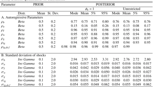
Table II - B Priors and Posteriors of Shocks parameters 1969Q1-2008Q3
Utility Channelspecification vs. Unrestricted
Parameter PRIOR POSTERIOR
φk=1 Unrestricted
Distr. Mean St. Dev. Mode Mean 5% 95% Mode Mean 5% 95% A. Autoregressive Parameters
ρb Beta 0.5 0.2 0.77 0.75 0.71 0.80 0.76 0.76 0.75 0.76
ρa Beta 0.5 0.2 0.15 0.16 0.05 0.26 0.15 0.13 0.08 0.17
ρI Beta 0.5 0.2 0.96 0.95 0.91 0.98 0.95 0.95 0.94 0.95
ρw Beta 0.5 0.2 0.95 0.93 0.88 0.98 0.95 0.95 0.94 0.96
ρg Beta 0.5 0.2 0.97 0.97 0.96 0.99 0.97 0.98 0.93 0.97
ρig Beta 0.5 0.2 0.94 0.90 0.91 0.98 0.95 0.94 0.93 0.95
ρig,de f Beta 0.5 0.2 0.98 0.98 0.96 0.99 0.98 0.97 0.99
B. Standard deviation of shocks
σb Inv Gamma 0.1 2.0 2.94 2.93 2.53 3.31 2.92 2.76 2.72 2.80
σa Inv Gamma 0.1 2.0 0.016 0.017 0.015 0.019 0.017 0.016 0.016 0.017
σI Inv Gamma 0.1 2.0 0.042 0.042 0.029 0.056 0.040 0.039 0.036 0.042
σw Inv Gamma 0.1 2.0 0.026 0.034 0.020 0.050 0.025 0.026 0.025 0.027
σg Inv Gamma 0.1 2.0 0.015 0.015 0.014 0.017 0.015 0.015 0.015 0.016
σig Inv Gamma 0.1 2.0 0.030 0.031 0.029 0.033 0.030 0.03 0.029 0.030
σig,de f Inv Gamma 0.1 2.0 0.054 0.055 0.048 0.062 0.054 0.055 0.049 0.062
Appendix C: Equilibrium Conditions with Transformed Variables
Equilibrium conditions follow from the first order conditions (F.O.C.s) of households’ and firms’ problems while imposing symmetry, fiscal policy equations, market clearing conditions and processes for the exogenous processes. VariablesCt,It,Kt,Wt,T axt,Tt,Gt,Igt,I
g,de f
t andBtare divided by the
level of technology,At. Lower case letters indicate transformed variables. The same treatment is
re-quired for the Lagrange multipliers associated with the budget constraint and the capital accumulation equation, respectivelyλt andqt(Tobin’s q).
• Consumption F.O.C.:
(1+τc)λtexp(−(γ+εat))=eεbt
φ ect
ct
!1 vh
ectexp(γ+εat)−γect−1−1 i
(19)
• Aggregator (consumption): ect=
φ(ct) v−1
v +(1−φ) (gt) v−1
v
v v−1
(20)
• Labor supply F.O.C.: λt=
χLσn t
(1−τw)w t
(21)
• Risk free asset F.O.C.: βEt
"
λt+1
λt
exp(−(γ+εat+1))(1+rt)
#
• Investment F.O.C.:
λt=λtqtEt
1−κ
2 e
εtIitexp(γ+ε a
t)
it−1
−eγ !2
− it
it−1
exp(γ+εat)κeεtI eεtIitexp(γ+ε a
t)
it−1
−eγ!+
(23) +βEt
λt+1qt+1exp(−(γ+εat+1)) e εI
t+1it+1
exp(γ+εat+1) it
!2
κeεIt+1 eεit+1it+1
exp(γ+εat+1) it
−eγ!
• Next period capital F.O.C.:
λtqt=Et
h
βλt+1exp(−(γ+εat+1))r
k
t+1ut+1−a(ut+1)](1−τ
k)+q
t+1(1−δ)
i
(24) wherea(ut)=γ1(ut−1)+γ22(ut−1)2represents the cost of using capital at intensityut.
• Capital law of motion:
kt+1=(1−δ)ktexp(−(γ+εat))+it
1−κ
2 e εI
titexp(γ+ε a
t)
it−1
−eγ !2
(25)
• Capacity utilization F.O.C.: rk
t =a′(ut)=γ1+γ2(ut−1) (26)
• MRS consumption/labor: mrst=eε
b
t χL
σn t
(1+τc)λ t
(27)
• Wage markup: 1+λw,t=
wt(1−τw)
mrst
(28) 1+λw,t=wt(1−τ
i
t)
mrst
(29)
• Production function:
yt=exp(−α(γ+εat))ekαt(Lt)1−α)−Φ (30)
• Aggregator (capital):
ekt=
"
φ(kt) vk−1
vk +(1−φ) (kg
t)
vk−1 vk
# vk vk−1
(31)
• Factor demands:
(1−α) yt Lt(1+λp,ss)
=wt (32) α
yt
ekt(1+λp,ss)
exp(γ+εat)φk
ekkt
t 1 vk
=rkt (33)
• Marginal cost:
MCt=
rktαw1t−α
αα(1−α)1−αφ
k e kt kt 1 vk
(KtG,de f)θg,de f
(34)
• Price markup:
1 MCt
• Evolution of the productivity of public capital:
KtG+1=(1−δKg)KtG+ξigt (36) whereξigt =igt/yt=exp(εigt +ssig)/(1+exp(ε
ig
t +ssig)) andssig=log(ξig,ss/(1−ξig,ss))
KtG+,1de f =(1−δKg,de f)KtG,de f+ξtig,de f (37) whereξigt ,de f=igt,de f/yt=exp(εigt ,de f+ssig,de f)/(1+exp(ε
ig,de f
t +ssig,de f)) andssig,de f=log(ξig,de f,ss/(1−
ξig,de f,ss))
• Government consumption:
ξtg=gt/yt=exp(εgt +ssg)/(1+exp(ε g
t +ssg)) (38)
wheressg=log(ξg,ss/(1−ξg,ss))
• Fiscal Rules:
bτit=ρτbτit−1+(1−ρτ)γτbrbt−4+ετt (39)
b
Tt=ρzTbt−1+(1−ρz)γzbrbt−1+εzt
• Government budget:
– Balanced:
τcct+τwwtLt+τk
h
rtkut−a(ut)
i
kt+tt=ξtgyt+ξtigyt+ξtig,de fyt (40) – Fiscal Strategy Model:
τcct+τit
wtLt+
h
rtkut−a(ut)
i
kt)+tt+(1+rbt)bt−1=bt+ξgtyt+ξtigyt (41)
• Shocks processes: εbt =ρbεbt−1+ηbt (42)
εIt =ρiεIt−1+ηIt
εat =ρaεat−1+ηat
εgt =ρgεgt−1+ηgt
εigt =ρigεiigt−1+ηigt
ετt =ρτεiτt−1+ητt
εTt =ρTεiTt−1+ηTt
εigt ,de f =ρig,de fεiigt−,1de f+ηigt ,de f
λw,t=(1−ρw)λw,ss+ρwλw,t−1+ηwt
Appendix D: Data Description
Tables bellow summarize the data and notation for the observed variables. Azevedo and Ercolani (2012) followed Smets and Wouters (2007).
Variable Designation Source CODE
Gross Domestic Product (Nominal) GDP U.S. Dep. of Commerce - BEA A191RC1 Personal Cons. Expenditures (Nominal) C U.S. Dep. of Commerce - BEA DPCERC1 Personal Cons.Expenditures - Durables (Nominal) Durables U.S. Dep. of Commerce - BEA DDURRC1 Private Fixed Domestic Investment (Nominal) PFI U.S. Dep. of Commerce - BEA A007RC1 Federal Cons. Expenditures (Nominal) G_Federal U.S. Dep. of Commerce - BEA A957RC1 State & Local Cons. Expenditures (Nominal) G_StateLocal U.S. Dep. of Commerce - BEA A991RC1 State & Local Gross Investment (Nominal) IG_StateLocal U.S. Dep. of Commerce - BEA A799RC1 Gross Domestic Product Deflator GDPDEF U.S. Dep. of Commerce - BEA GDPDEF Hourly Compensation, Non Farm Sector (Nominal) Wages Bureau of Labor Statistics PRS85006103 Civilian noninstitutional population, 16 years and over POPULATION Bureau of Labor Statistics LNU00000000Q
Table II -D - Observables for measurement equations
Ytobs=(GDP/GDPDEF)/POPULATION
Cobs
t =((C-Durables)/GDPDEF)/POPULATION
Iobs
t =((PFI+Durables)/GDPDEF)/POPULATION Wtobs=(Wages/GDPDEF)/POPULATION
ξgt,obs=(G_Federal+G_StateLocal)/GDP