Insper and NOVA School of Business and Economics
Double Degree Masters in Economics Program
Bruno Jordan Orfei Abe
Insper: 110168141
NOVA SBE: 770
BRAZILIAN EQUITY RISK PREMIUM ANALYSIS:
A MACROECONOMIC APPROACH
São
Paulo / Lisbon
Bruno Jordan Orfei Abe
BRAZILIAN EQUITY RISK PREMIUM ANALYSIS:
A MACROECONOMIC APPROACH
Work Project presented to the Double Degree Masters in Economics Program from Insper and NOVA School of Business and Economics as a part of the pre requisites for the entitlement as Master in Economics.
Area of Expertise: Macrofinance
Advisor: Prof. Dr. Ricardo Dias de Oliveira Brito
Co-Advisor: Prof. Dr. Andre C. Silva
São Paulo / Lisbon
Abe, Bruno Jordan Orfei
Brazilian Equity Risk Premium Analysis: A Macroeconomic Approach/Bruno Jordan Orfei Abe; Advisor: Prof. Dr. Ricardo Dias de Oliveira Brito; Co-Advisor: Prof. Dr. André C. Silva. – Lisboa: Universidade Nova de Lisboa 2014.
Work Project (Masters – Masters in Economics. Area of expertise: Macrofinance) – Insper Instituto de Ensino e Pesquisa and NOVA School of Business and Economics.
APPROVAL SHEET
Bruno Jordan Orfei Abe
Brazilian Equity Risk Premium Analysis: A Macroeconomic Approach
Work Project presented to the Double Degree Masters in Economics Program from Insper and NOVA School of Business and Economics as a part of the pre requisites for the entitlement as Master in Economics. Area of Expertise: Macrofinance
Approved in: January, 2015
Committee
Prof. Dr. Ricardo Dias de Oliveira Brito
Institution: Insper Signature:
Prof. Dr. André C. Silva
Institution: NOVA SBE Signature:
Prof. Dr. Marco Lyrio
Institution: Insper Signature:
Prof. Dr. José Tavares
ABSTRACT
Abe, Bruno Jordan Orfei. Brazilian Equity Risk Premium Analysis: A Macroeconomic Approach. Master’s Thesis – Insper, São Paulo, 2015 and NOVA School of Business and Economics, Lisbon, 2015.
This research studies the role of fluctuations in the aggregate consumption-wealth
ratio 𝑐𝑎𝑦 proposed by Lettau and Ludvigson (2001) as a predictor of stock returns in the Brazilian economy. Using quarterly data, evidence for predictability of asset growth was
found with an 𝑅̅2of over 45% and a highly significant coefficient as expected, in contrast
to absence of statistical evidence for predictability of stock returns or excess returns.
Regressions containing those fluctuations also resulted in worse 𝑅̅2. For the data used,
dividend yield was not capable of showing predictive power also. The predictability of the
returns on the Brazilian economy is not rejected but data fails to show the expected
results. Finding macroeconomic data that represent the same agent was a big obstacle.
After testing many different datasets and different model specifications, data still failed to
show any explanatory power over returns or excess returns.
Summary
1. Introduction ... 6
2. Model and Methodology ... 8
2.1. The Consumption-Wealth Ratio ... 8
2.2. Dynamic Dividend Growth Model ... 11
3. Data ... 12
3.1. Population ... 12
3.2. Consumption and Labor Income ... 13
3.3. Asset Holdings ... 14
4.4.1 Real Estate ... 15
4.4.2 Financial Assets ... 16
4. Results ... 16
1. Introduction
A fundamental discussion in finance is how predictable are stock returns and what
drives its intertemporal variation. Over the past years researchers tried to find and improve
explanatory power for models willing to accomplish that objective. The capital asset pricing
model (CAPM) of Sharpe (1964) and Lintner (1965) marks the birth of asset pricing theory
as the first coherent framework to answer part of this question. As this theory was later
proven inconsistent with numerous empirical regularities as in Basu (1977), Banz (1981),
Shanken (1985), and Fama and French (1992, 1993), asset pricing theory has fallen on
hard times. Why has the CAPM failed? One possibility is that its framework fails to account
for effects of time-varying investment opportunities in the calculation of an asset’s risk. In response to this failure, intertemporal asset pricing models, such as the most
prominent of them, the consumption CAPM (CCAPM) developed by Breeden (1979),
initially tried to remedy this defect. Unfortunately, these models also proved disappointing
empirically as in Hansen and Singleton (1982, 1983), Mankiw and Shapiro (1986),
Breeden, Gibbons, and Litzenberger (1989), Campbell (1996), and Cochrane (1996). The
results presented by these researches suggest that both the CAPM and the CCAPM may
have inadequate allowances for time variation in the conditional moments of returns.
Lettau and Ludvigson (2001) explore a conditional version of the consumption
CAPM. They try to express the stochastic discount factor not as an unconditional linear
model, as in traditional derivations of the CCAPM, but as a conditional, or scaled, factor
model. As they discuss, conditioning the model improves the fit of the CCAPM because
some stocks are highly correlated with growth in consumption in bad times, or when the
risk aversion is high, than in the good times, when the risk aversion is low. In their model,
they were able to argue that their results go a long way toward resolving this controversy
and show that the scaled multifactor version of the CCAPM can explain a substantial
fraction of the cross-sectional variation in average returns on stock portfolios sorted
according to size and book-to-market equity ratios.
Their results helped shedding the light on why the three-factor model by Fama and
French (1996) had performed so well relatively to the unscaled size: while analyzing the
data they figure that the Fama-French factors are somehow mimicking portfolios for risk
In addition to that, expected excess returns on common stocks appear to vary with
the business cycle, which suggests that stock returns should be forecastable by business
cycle variables at cyclical frequencies. Financial indicators such as the ratios of price to
dividends, price to earnings, or dividend to earnings have been most successful at
predicting returns, Fama and French (1988) argues that the power of dividend yields to
forecast stock returns increases with return horizon. Campbell (1991), and Campbell, Lo,
and MacKinlay (1997) show that this variable performs better in horizons that excess two
years. Lettau and Ludvigson (2001) conclude that, for the U.S market, the
consumption-wealth ratio was able to add significantly explanatory power to most of the models
discussed above.
This article follows Lettau and Ludvigson (2001) applying their micro-founded
model that uses the consumption-aggregate wealth ratio 𝑐𝑎𝑦 as a proxy for the
intertemporal trade-off in investment opportunities to the Brazilian stock market in order
to check if the same results are found when the model is exposed to another economy.
To accomplish that objective, it explains the assumptions and mechanics of the model
framework and discuss its performance while applied to the Brazilian stock market, also
when compared with other disseminated models.
The rest of the paper is organized as follows. The next section replicates the
framework Lettau and Ludvigson (2001) used on their model showing the link between
consumption, aggregate wealth, and expected returns, and how they express the
important predictive components of the consumption-aggregate wealth ratio in terms of
observable variables. Section three shows how this research managed to deal with the
required time series to replicate their study for the Brazilian market. Section four
documents the main findings on the predictability of stock returns while the model is
2. Model and Methodology
2.1. The Consumption-Wealth Ratio
This section replicates and analyzes the model Lettau and Ludvigson (2001) used
to present a general framework linking consumption, asset holdings, and labor income
with expected returns. The authors use a micro-founded model that studies a
representative agent and its choices while consuming or investing its wealth and income.
Consider a representative agent economy in which all wealth, including human
capital is tradable. Let 𝑊𝑡 be the aggregate wealth (human capital plus asset holdings) in period 𝑡. 𝐶𝑡 is the consumption and 𝑅𝑤,𝑡+1 is the net return on aggregate wealth. The accumulation equation for aggregate wealth may be written1
𝑊𝑡+1 = (1 + 𝑅𝑤,𝑡+1)(𝑊𝑡− 𝐶𝑡) (1)
They define r ≡ log(1 + 𝑅), and use lowercase letters to denote log variables throughout. Campbell and Mankiw (1989) show that, if the consumption-aggregate wealth
ratio is stationary, the budget constraint may be approximated by taking a first-order Taylor
expansion of the equation. The resulting approximation gives an expression for the log
differences in aggregate wealth
∆𝑤𝑡+1≈ 𝑘 + 𝑟𝑤,𝑡+1(1 − 1 𝜌⁄ )(𝑐𝑤 𝑡− 𝑤𝑡) (2)
where 𝜌𝑤 is the steady-state ratio of new investment to total wealth, (𝑊 − 𝐶)/𝑊, and 𝑘 is a constant that plays no role in their analysis.2 Solving this difference equation forward
and imposing that lim
𝑖→∞𝜌𝑤 𝑖 (𝑐
𝑡+1− 𝑤𝑡+1) = 0, the log consumption-wealth ratio may be
written
1 Labor income does not appear explicitly in this equation because of the assumption that the market value of tradable human capital is included in aggregate wealth.
𝑐𝑡− 𝑤𝑡 = ∑ 𝜌𝑤𝑖 (𝑟𝑤,𝑡+𝑖− ∆𝑐𝑡+𝑖) ∞
𝑖=1
(3)
This equation holds simply as a consequence of the agent’s intertemporal budget
constraint and therefore holds ex post, but it also holds ex ante. Accordingly, we can take
conditional expectations of both sides of it to obtain
𝑐𝑡− 𝑤𝑡 = 𝐸𝑡∑ 𝜌𝑤𝑖 (𝑟𝑤,𝑡+𝑖− ∆𝑐𝑡+𝑖) ∞
𝑖=1
(4)
where 𝐸𝑡 is the expectation operator conditional on information available at time 𝑡. This equation shows that, if the aggregate consumption-wealth ratio is not constant, it must
either forecast changing returns on the market portfolio or changing consumption growth.
Put another way, as the equation (4) shows, the aggregated consumption-wealth ratio can
only vary if consumption growth or returns or both of them are predictable.
The aggregate consumption-wealth ratio is a function of expected future returns for
the market portfolio in a broad range of optimal consumption models. The information set
upon which expectations are conditioned will depend on the state variables in the model.
These models may differ in their specification or preferences, or in the assumptions about
the stochastic properties of consumption properties of consumption and asset returns. All
of them, however, will imply that the consumption-aggregate wealth ratio is a function of
expected future returns, and that agents’ expectations about future returns and
consumption growth may be inferred from observable consumption behavior. Moreover,
there is no need to explicitly model how returns to wealth and consumption growth are
determined by some specific set of preferences.
Because aggregate wealth, in particular, human capital, is not observable, the
framework presented above is not directly suited for predicting asset returns. To overcome
this obstacle, assumptions about the nonstationary component of human capital,
𝑧𝑡, where 𝑘 is a constant and 𝑧𝑡 is a mean zero stationary random variable. As shown by
the authors in many models linking labor income to the stock of human capital, the log of
aggregate labor income captures the nonstationary component of human capital.
Let 𝐴𝑡 be the asset holdings, and let 1 + 𝑅𝑎,𝑡 be its gross return. Aggregate wealth is therefore 𝑊𝑡 = 𝐴𝑡+ 𝐻𝑡 and log aggregate wealth may be approximated as
𝑤𝑡 = 𝜔𝑎𝑡+ (1 − 𝜔)ℎ𝑡 (5)
Where 𝜔 equals the average share of asset holdings in total wealth, 𝐴 𝑊⁄ . This ratio may also be expressed in terms of the steady-state labor income and returns as
𝑅ℎ𝐴 (𝑌 + 𝑅⁄ ℎ𝐴).
The return to aggregate wealth can be decomposed into the returns of its two
components
1 + 𝑅𝑤,𝑡 = 𝜔𝑡(1 + 𝑅𝑎,𝑡) + (1 − 𝜔𝑡)(1 − 𝑅ℎ,𝑡). (6)
Campbell (1996) shows that (6) may be transformed into an approximate equation for log
returns taking the form
𝑟𝑤,𝑡 ≈ 𝜔𝑟𝑎,𝑡+ (1 − 𝜔)𝑟ℎ,𝑡. (7)
Substituting (7) into the budget constraint (4) results in
𝑐𝑡− 𝜔𝑎𝑡− (1 − 𝜔)ℎ𝑡= 𝐸𝑡∑ 𝜌𝑤𝑖 {[𝜔𝑟𝑎,𝑡+𝑖+ (1 − 𝜔)𝑟ℎ,𝑡+𝑖] − ∆𝑐𝑡+𝑖} ∞
𝑖=1
This equation still contains the unobservable variable ℎ𝑡, on the left-hand side. To remove it, we substitute ℎ𝑡 = 𝑘 + 𝑦𝑡+ 𝑧𝑡 into (8), which yields an approximate equation describing the log consumption-aggregate wealth ratio using only observable variables on the left
hand side:
𝑐𝑡− 𝜔𝑎𝑡− (1 − 𝜔)𝑦𝑡 = 𝐸𝑡∑ 𝜌𝑤𝑖 {[𝜔𝑟𝑎,𝑡+𝑖+ (1 − 𝜔)𝑟ℎ,𝑡+𝑖] − ∆𝑐𝑡+𝑖} + (1 − 𝜔)𝑧𝑡 ∞
𝑖=1
. (9)
Since all the terms on the right-hand side of (9) are presumed stationary, for this
equality to hold, 𝑐, 𝑎, and 𝑦 must be cointegrated, and the left-hand side of (9) gives the deviation in the common trend of 𝑐𝑡, 𝑎𝑡, and 𝑦𝑡. In what follows, the trend deviation term
𝑐𝑡− 𝜔𝑎𝑡− (1 − 𝜔)𝑦𝑡 is denoted as 𝑐𝑎𝑦𝑡. Moreover, equation (9) shows that 𝑐𝑎𝑦𝑡 will be a
good proxy for market expectations of future asset returns 𝑟𝑎,𝑡+𝑖as long as expected future returns on human capital, 𝑟ℎ,𝑡+𝑖, and consumption growth, ∆𝑐𝑡+𝑖, are not too variable, or as long as these variables are highly correlated with expected returns on assets.
2.2. Dynamic Dividend Growth Model
It is instructive to compare (9) to an expression for another variable that has been
widely used to forecast asset returns, the log dividend-price ratio. Let 𝑑𝑡 and 𝑝𝑡 be the log dividend and log price, respectively, of the stock of asset wealth. Campbell and Shiller
(1988) show that the log dividend-price ratio may be written
𝑑𝑡− 𝑝𝑡= 𝐸𝑡∑ 𝜌𝑎𝑖(𝑟𝑎,𝑡+𝑖− ∆𝑑𝑡+𝑖) ∞
𝑖=1
. (10)
where 𝜌𝑎 = 𝑃 (𝑃 + 𝐷)⁄ . This equation is derived by taking a first-order Taylor approximation of the equation defining the log stock return, 𝑟𝑡= log(𝑃𝑡+ 𝐷𝑡) − log(𝑃𝑡). Put in another way, if the dividend-price ratio is high, agents must be expecting either high
Note the similarity between (10) and (4). The role of consumption in (4) is directly
analogous to that of 𝑑𝑡 in (10): when the consumption-aggregate wealth ratio is high, agents must be expecting either high returns on the market portfolio in the future or low
consumption growth rates.
3. Data
Lettau and Ludvigson (2001) rely on existing data series for the U.S. market in
order to compose the 𝑐𝑎𝑦 index: aggregate consumption, asset holdings, and labor income. For the aggregate consumption, they use data for consumption of nondurable
goods and services, excluding clothing and shoes articles. For the labor income, they
combine a set of factors to generate the model that they believe are the most realistic one
to replicate reality about that information. Data for these series come from the Bureau of
Economic Analysis. Finally, for the household wealth, they use data provided by the
Federal Reserve. All series at quarterly frequency.
To generate comparable results, in this article, prices are expressed in Brazilian
Reais from 1996, deflated by the index IGP-DI3. Series were chosen aiming to
approximate the observed series by the same representative agent. This section show
information used for the estimation of the best model found.
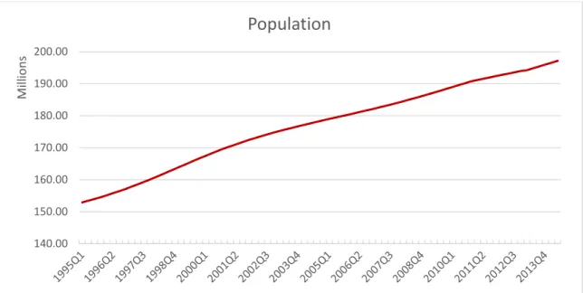
3.1. Population
The population series are from IPEA Data, although, the original provider for this
information is the Brazilian Institute of Geography and Statistics (IBGE). The available
series is annual and it was broken in quarters by an exponential interpolation method
vertex by vertex. As population data are available only until the last quarter of 2012, an
extrapolation procedure was used on the data by using a simple linear trend equation for
the last information (the linear trend equation seemed to be a realistic representative of
the data for the short run).
Figure 1 - Quarterly Population Series in millions of habitants from 1995Q1 - 2014Q2
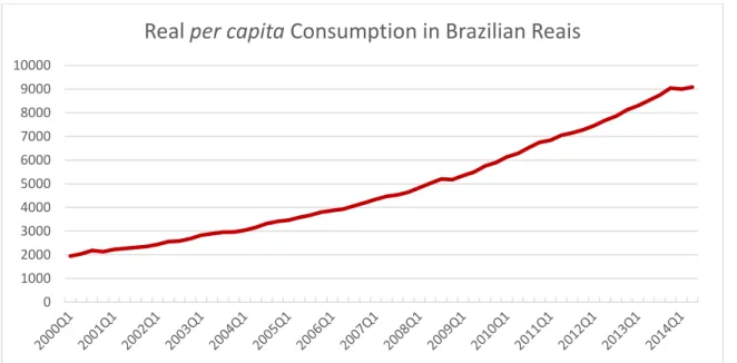
3.2. Consumption and Labor Income
Consumption is the Final Consumption Expenditures and labor income is the Gross
National Disposable Income from the quarterly economic account available with the GDP
decomposition on the complimentary tables, provided by IBGE. This is the best pair of
aggregated information available that represent the same individual. Consumption
contains information about durable goods and it should not, given that these expenditures
represent additions to capital stock and not the flow of capital. Unfortunately, there is no
information available to decompose this series and get only expenditures with non-durable
goods and services. Both series were seasonally adjusted with a Census X12 filter. With
this adjustment, it is expected that the ratio of the share of durable and non-durable goods
in total consumption become more static, diminishing the problem of using this series as
an indicator for the consumption flow. Other macroeconomic series were tested to check
the validity of this choice but all of them generated worse results. Further discussion
containing the other series is in the Results section.
140.00 150.00 160.00 170.00 180.00 190.00 200.00
Mi
ll
ion
s
Figure 2 – Quarterly Seasonally Adjusted Real per capita Consumption in Brazilian Reais from 2000Q1 - 2014Q2
Figure 3 – Quarterly Seasonally Adjusted Real per capita Labor Income in Brazilian Reais from 2000Q1 - 2014Q2
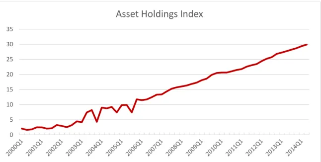
3.3. Asset Holdings
The concept asset holdings is not commonly used in Brazilian literature, as a
consequence, institutional data providers lack to provide this information. There is no
decomposition of the household net worth available. A proxy portfolio containing three
weighted components: real estate, risk free assets, and risky assets, stands for this
information. 0 1000 2000 3000 4000 5000 6000 7000 8000 9000 10000
Real
per capita
Consumption in Brazilian Reais
0 2000 4000 6000 8000 10000 12000
Figure 4 - Asset holdings index from 2000Q1 - 2014Q2
The U.S. household decomposition was the benchmark for the weights used in this
portfolio, approximately 90% of the asset holdings derive from real estate assets, 5% from
risky assets and 5% from risk free assets. More information about each component of this
portfolio is in the next subsections.
4.4.1 Real Estate
The literature suggests that land and building taxes capture variations on the real
estate value. As explored by de Carvalho Jr. (2009), this relationship is not trustable for
Brazil, and the main reason for this fact is that a significant part of the population (in
general the poor population) does not report how much they have to pay for it. Additionally,
the available information for this tax is still too short to enter in our model. To overcome
this difficulty, a private database containing information about many São Paulo’s real
estate assets valuated by a specialized company was used to replicate movements in the
market4. Real estate information for the whole country is not available and as only the
agents that are able to smooth consumption are the focus of the study, this series is the
best representation of their real estate component.
4 I thank Eribaldo Ximenes for providing the worked real estate time series containing information about São Paulo’s real estate market created using the database from Engebanc that contains valuation information for many real estate assets.
0 5 10 15 20 25 30 35
4.4.2 Financial Assets
The perfect representation of the Brazilian market portfolio is almost impossible.
Literature usually relies on the Ibovespa index as a representation of it. Considering that
a small part of the Brazilian population have access to the stock market and the Ibovespa
index weights stocks using trading volume, for the purpose of this study, it is not the best
option. A portfolio that gives more weight to small companies that are traded on the stock
market would better represent all the companies that compose the Brazilian market
portfolio. Using Economatica data for all companies that have common or preferred stocks
traded since January 1st, 1986 until June 30th, 2014 it is possible to create an equally
weighted portfolio index5 and to create a dividend-price series for it. This index represents
the 5% that stands for risky assets. In regressions, excess returns are
the 𝐸𝑞𝑢𝑎𝑙𝑙𝑦 𝑊𝑒𝑖𝑔ℎ𝑡𝑒𝑑 𝑃𝑜𝑟𝑡𝑓𝑜𝑙𝑖𝑜 𝑅𝑒𝑡𝑢𝑟𝑛 − 𝑆𝐸𝐿𝐼𝐶 𝑅𝑒𝑡𝑢𝑟𝑛.
The risk free assets series contains 95% of government bonds that are the
Government Debt Public Bonds issued by the National Treasury from the Brazilian Central
Bank, and 5% savings account that are the saving accounts stock series from the Brazilian
Central Bank. This series represent the last 5% of the asset holdings series that stands
for risk free assets.
4. Results
The first important task while using 𝑐𝑎𝑦 to forecast asset returns is the estimation of the parameters of the shared trend in consumption, asset holdings, and labor income.
Although these three variables are assumed endogenously determined, the asymptotic
properties of cointegrated variables can avoid this difficulty.
Testing for cointegration, requires that all variables are integrated of the same
order. Summary for the unit root tests are on the table below for each variable shows that
all the variables are integrated of first order I(1).
Unit Root Test Summary
(Results are p-value for ADF tests where null hypothesis indicates a unit root)
log(𝐶𝑜𝑛𝑠𝑢𝑚𝑝𝑡𝑖𝑜𝑛) log(𝐴𝑠𝑠𝑒𝑡 𝐻𝑜𝑙𝑑𝑖𝑛𝑔𝑠) log(𝐿𝑎𝑏𝑜𝑟 𝐼𝑛𝑐𝑜𝑚𝑒)
Level 1st Difference Level 1st Difference Level 1st Difference
0.6331 0.0000 0.9988 0.0000 0.8828 0.0001
Table 1 – ADF unity root test summary for all variables composing cay in level and first difference.
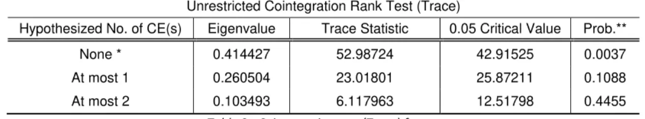
The Johansen cointegration test is highly sensitive to lag specification when
exposed to small samples. This research considers mainly two factors to determine the
number of lags for the models. The first one is statistic, relying on the information criteria;
the second one is economic, considering the business cycles. The information criteria
pointed to the use of a one lag model. Since data is quarterly, and sample is really small,
a one lag VAR6 was estimated and the Johansen cointegration test was applied, indicating
the existence of one cointegration equation between the series. Table 2 and Table 3 show
results for these tests. They indicate that the three components do share a common
long-term trend. How can deviations from this shared trend be interpreted to check if they are
better described as transitory movements in asset wealth or as transitory movements in
consumption and labor income?
Unrestricted Cointegration Rank Test (Trace)
Hypothesized No. of CE(s) Eigenvalue Trace Statistic 0.05 Critical Value Prob.**
None * 0.414427 52.98724 42.91525 0.0037
At most 1 0.260504 23.01801 25.87211 0.1088
At most 2 0.103493 6.117963 12.51798 0.4455
Table 2 - Cointegration test (Trace) for cay
Unrestricted Cointegration Rank Test (Maximum Eigenvalue)
Hypothesized No. of CE(s) Eigenvalue Max-Eigen Statistic 0.05 Critical Value Prob.**
None * 0.414427 29.96923 25.82321 0.0134
At most 1 0.260504 16.90005 19.38704 0.1108
At most 2 0.103493 6.117963 12.51798 0.4455
Table 3 - Cointegration test (Maximum Eigenvalue) for cay
To answer this question, it is instructive to examine the error correction term of a
vector error correction model where log difference in consumption, asset wealth, and labor
income are each regressed on their own lags, also including this cointegration equation.
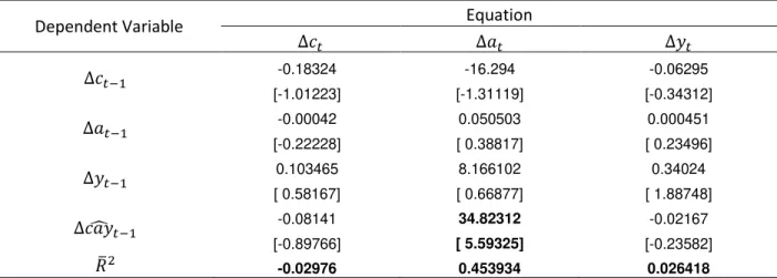
Table 4 presents a summary of this result.
Focusing on the relationship between the estimated trend deviation 𝑐𝑎𝑦̂𝑡−1 and future growth rates of each variable reveals an interesting property of the data on the three
components. As showed in the revision of the framework proposed by Lettau and
Ludvigson (2001), estimation of the asset growth equation shows that 𝑐𝑎𝑦̂𝑡−1 predicts asset growth, implying that deviations in asset wealth from its shared trend with labor
income and consumption uncover important transitory variation in asset. With this in
hands, the focus now is showing that this variable predicts asset growth because the
estimated trend deviation forecasts asset returns.
Dependent Variable Equation
∆𝑐𝑡 ∆𝑎𝑡 ∆𝑦𝑡
∆𝑐𝑡−1 -0.18324 -16.294 -0.06295
[-1.01223] [-1.31119] [-0.34312]
∆𝑎𝑡−1 -0.00042 0.050503 0.000451
[-0.22228] [ 0.38817] [ 0.23496]
∆𝑦𝑡−1 0.103465 8.166102 0.34024
[ 0.58167] [ 0.66877] [ 1.88748]
∆𝑐𝑎𝑦̂𝑡−1 -0.08141 34.82312 -0.02167
[-0.89766] [ 5.59325] [-0.23582]
𝑅̅2 -0.02976 0.453934 0.026418
Table 4 - Estimates from the VECM for the coefficients of the column variable on the row variable, t-statistics appear in brackets. Statistically significant coefficients are bold.
The financial data include stock returns and the dividend-price ratio, Table 5 below
shows some statistics for all this data and also for the trend deviation term 𝑐𝑎𝑦̂𝑡 for the biggest common sample available. Focusing on the discussion on the estimated trend
deviation 𝑐𝑎𝑦̂ , results presented in the summary table are discouraging. This variable is negatively correlated to the excess stock returns. Additionally it is well known that the
price-dividend yield should be very persistent, and for our sample, it does not show that7.
𝑟𝑚− 𝑟𝑓,𝑡 𝑑 𝑡− 𝑝𝑡 𝑐𝑎𝑦̂𝑡 Panel A: Correlation Matrix
𝑟𝑚− 𝑟𝑓,𝑡 1.0000 -0.0587 -0.0509
𝑑 𝑡− 𝑝𝑡 1.0000 0.0324
𝑐𝑎𝑦̂𝑡 1.0000
Panel B: Univariate Summary Statistics
Mean -0.0094 0.0072 0.0000
𝜎 0.0384 0.0031 0.0296
Autocorrelation 0.3150 -0.0240 0.0200
Table 5 - Summary statistics for financial data.
The 𝑐𝑎𝑦̂ also shows a small autocorrelation. Lettau and Ludvigson (2001) show that autocorrelation for their trend deviation term is lower than the dividend-price ratio but
not as low as the ones found with data for Brazil. This affects the forecasting equations,
removing the inference problems that exists for estimations with big autocorrelations as it
would be expected from the dividend yield.
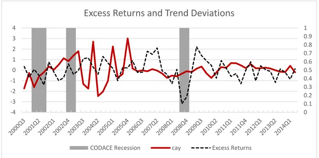
Figure 5 - Standardized cay series with Equally Weighted Portfolio Excess Returns
Figure 5 plots the standardized excess returns paired with the trend deviation. The
𝑐𝑎𝑦 ratio does not seem to work well while predicting changes on the excess returns. At some periods this relation holds, but fails at most others as in 2004Q1, for example, we
see deviations showing an upcoming raise on the excess returns, but on the right next 0 0.1 0.2 0.3 0.4 0.5 0.6 0.7 0.8 0.9 1 -4 -3 -2 -1 0 1 2 3 4
Excess Returns and Trend Deviations
quarter, they lower. Predictive powers seems to get even worse within the CODACE8
recession indicator. Most of the spikes found in the excess returns are not forecasted by
the trend deviations.
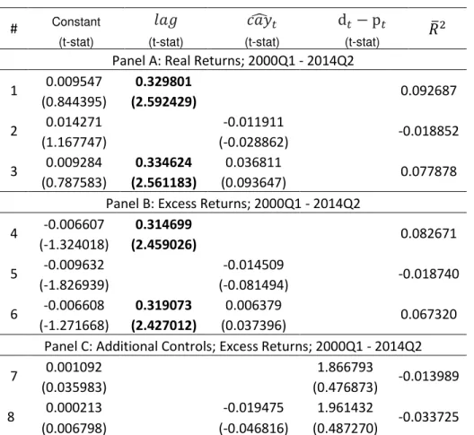
Moving on to assess the forecasting power of detrended wealth for asset returns,
Table 6 show a set of results using the lagged trend deviation, 𝑐𝑎𝑦̂𝑡−1, as a predictive variable for returns and excess returns. All regressions use the equally weighted portfolio
as the benchmark for stock returns. For all the equations, the lagged variable is the only
statistically significant, when present. The most relevant finding is that, for this sample,
the lagged trend deviations are not statistically significant, showing absolute t-statistic
values far below the expected 2. These findings go in the opposite direction as the ones
from Lettau and Ludvigson (2001). Models using 𝑐𝑎𝑦̂𝑡−1 as explanatory variable also diminishes the 𝑅̅2 of the regressions. Data show that, for the chosen samples and set of
information, 𝑐𝑎𝑦̂ is neither a good predictor for real returns nor excess returns in Brazil. What could have generated these results? As Lettau and Ludvigson (2001) say, using
aggregate data in all analyses would most likely bias downward the forecasting power of
the 𝑐𝑎𝑦𝑡, especially because it is known that there is a limited participation in asset markets for the population, but this also affects the model estimated for the U.S. market.
On the other hand, the dividend-price ratio from the equally weighted portfolio does
not show explanatory power, this goes also against Shiller (1984), Campbell and Shiller
(1988), and Fama and French (1988) that find that the ratio of price to dividends have
predictive power for excess returns. Bhargava, Dania, and Malhotra (2011) show that this
ratio is statistically significant for Brazil, but they use monthly data for Ibovespa instead of
quarterly data for an equally weighted portfolio. Using quarterly Ibovespa returns as
explained variable instead of the equally weighted portfolio did not result in any better
estimation.
The most obvious difference between estimations for Brazil and for the U.S.
economy lay down in the information set available for each economy. Data for
consumption considers durable goods, which represent replacements or additions to
stock and not the flow of consumption. Unfortunately, it is not possible to determine which
part of it is attributable to durable goods and which is attributable to nondurables goods
and services. Additionally, the samples available are expressively smaller than the ones
available on the U.S. economy and used by Lettau and Ludvigson (2001). It is possible
that they do not capture the required variability for predicting returns as expected.
# Constant 𝑙𝑎𝑔 𝑐𝑎𝑦̂𝑡 d𝑡− p𝑡 𝑅̅2
(t-stat) (t-stat) (t-stat) (t-stat)
Panel A: Real Returns; 2000Q1 - 2014Q2
1 0.009547 0.329801 0.092687
(0.844395) (2.592429)
2 0.014271 -0.011911 -0.018852
(1.167747) (-0.028862)
3 0.009284 0.334624 0.036811 0.077878 (0.787583) (2.561183) (0.093647)
Panel B: Excess Returns; 2000Q1 - 2014Q2
4 -0.006607 0.314699 0.082671
(-1.324018) (2.459026)
5 -0.009632 -0.014509 -0.018740
(-1.826939) (-0.081494)
6 -0.006608 0.319073 0.006379 0.067320 (-1.271668) (2.427012) (0.037396)
Panel C: Additional Controls; Excess Returns; 2000Q1 - 2014Q2
7 0.001092 1.866793 -0.013989
(0.035983) (0.476873)
8 0.000213 -0.019475 1.961432 -0.033725 (0.006798) (-0.046816) (0.487270)
Table 6 - Estimates From OLS Regressions of Stock Returns on Lagged Variables Named at the Head of a Column.
Different datasets were tested to validate the samples used. Estimations with
average per capita labor income for metropolitan regions from 2001Q3 until 2014Q2 and
Gross Disposable Income from 1996Q1 until 2014Q2, both from IBGE as proxies for
income and Final Household Consumption, following the same time constraint from labor
income, from IBGE as proxy for consumption. All of them, in general, resulted in even
5. Conclusion
Investigating the conditions under which consumption, labor income and asset
holdings share a common long-run trend and that deviations from this trend can contain
information about time-varying investment opportunities and expectations about future
returns on the stock market led to testing the framework of the model developed by Lettau
and Ludvigson (2001).
The same methodology was replicated using the best available Brazilian time
series that represent the consumption, asset holdings and labor income, but facing some
limitations to find specific data and desired sample size. Representation to the same agent
while composing the three series explain difficulties for finding good information sets for
the Brazilian economy.
In the quest to overcome this difficulties, many models were estimated with different
specifications and different datasets, but all of them resulted in undesired lack of
explanation power while using 𝑐𝑎𝑦𝑡 as a predictor to returns or excess returns on the stock market. Effects from 𝑐𝑎𝑦𝑡 into the asset growth, although, are present in most of the estimated models.
The use of 𝑐𝑎𝑦𝑡 as a proxy to the intertemporal variation in the investment opportunities was not capable of adding explanation power to the regressions of real
returns or excess returns for the equally weighted portfolio. Dividend-price ratio series
also faced a lack of explanation power. Results force the belief that the samples used
were not able to account for the information needed to explicit the expected predictability.
Deeper research has to be done in order to create better proxies for the information,
maybe using other datasets that were not available for this work. A subset of information
emphasizing the population of metropolitan areas would also help to clear the data, as
they represent better the part of the population that has access to the stock markets and
also separate the part of the population that are able to smooth consumption as they do
References
Banz, RW 1981, 'THE RELATIONSHIP BETWEEN RETURN AND MARKET VALUE OF COMMON STOCKS', Journal Of Financial Economics, 9, 1, pp. 3-18
BASU, S 1977, 'INVESTMENT PERFORMANCE OF COMMON STOCKS IN RELATION TO THEIR PRICE-EARNINGS RATIOS: A TEST OF THE EFFICIENT MARKET HYPOTHESIS', Journal Of Finance, 32, 3, pp. 663-682
Bhargava, V, Dania, A, & Malhotra, D 2011, 'The Relationship between Price-Earnings Ratios, Dividend Yield, and Stock Prices: Evidence from BRIC Countries', Journal Of Emerging Markets, 16, 1, pp. 31-43
Black, F 1972, 'Capital Market Equilibrium with Restricted Borrowing', Journal Of Business, 45, 3, pp. 444-455
Breeden, DT 1979, 'An Intertemporal Asset Pricing Model with Stochastic Consumption and Investment Opportunities', Journal Of Financial Economics, 7, 3, pp. 265-296
BREEDEN, D, GIBBONS, M, & LITZENBERGER, R 1989, 'Empirical Tests of the Consumption-Oriented CAPM', Journal Of Finance, 44, 2, pp. 231-262
Campbell, JY 1996, 'Understanding risk and return', Journal Of Political Economy, 104, 2, p. 298
Campbell, J, Campbell, J, Shiller, R, & Shiller, R 1988, 'The dividend-price ratio and expectations of future dividends and discount factors', Review Of Financial Studies, 1, 3
Campbell, J, & Mankiw, N 1989, 'Consumption, Income, and Interest Rates: Reinterpreting the Time Series Evidence', NBER/Macroeconomics Annual (MIT Press), 4, 1, pp. 185-216
Cochrane, JH 1996, 'A Cross-Sectional Test of an Investment-Based Asset Pricing Model', Journal Of Political Economy, 104, 3, pp. 572-621
de Carvalho Jr., Pedro Humberto Bruno (2009) : Aspectos distributivos do IPTU e do patrimônio imobiliário das famílias brasileiras, Texto para Discussão, Instituto de Pesquisa Econômica Aplicada (IPEA), No. 1417
Duffie, D, & Zame, W 1989, 'THE CONSUMPTION-BASED CAPITAL ASSET PRICING MODEL', Econometrica, 57, 6, p. 1279
Enders, Walter. CHAPTER 5: Multiequation Time Series Models In: Enders, Walter. Title: Applied Econometric Time Series p. 313, 3rd edition. Publisher: John Wiley & Sons, Inc.
Fama, E, & French, K 1988, 'DIVIDEND YIELDS AND EXPECTED STOCK RETURNS', Journal Of Financial Economics, 22, 1, pp. 3-25
Fama, E, & French, K 1993, 'Common risk factors in the returns on stocks and bonds', Journal Of Financial Economics, 33, 1, pp. 3-56
Fama, E, & French, K 1996, 'Multifactor Explanations of Asset Pricing Anomalies', Journal Of Finance, 51, 1, pp. 55-84
Fama, Eugene F., and Kenneth R. French. 2004. "The Capital Asset Pricing Model: Theory and Evidence." Journal of Economic Perspectives, 18(3): 25-46.
GUO, H, WANG, Z, & YANG, J 2013, 'Time-Varying Risk-Return Trade-off in the Stock Market', Journal Of Money, Credit & Banking (Wiley-Blackwell), 45, 4, pp. 623-650
Hansen, L, & Singleton, K 1982, 'GENERALIZED INSTRUMENTAL VARIABLES ESTIMATION OF NONLINEAR RATIONAL EXPECTATIONS MODELS', Econometrica, 50, 5, pp. 1269-1286
Hansen, L, & Singleton, K 1983, 'Stochastic Consumption, Risk Aversion, and the Temporal Behavior of Asset Returns', Journal Of Political Economy, 91, 2, pp. 249-265
Jagannathan, R, & Zhenyu, W 1996, 'The Conditional CAPM and the Cross-Section of Expected Returns', Journal Of Finance, 51, 1, pp. 3-53
Lettau, M, & Ludvigson, S 2001, 'Consumption, Aggregate Wealth, and Expected Stock Returns', Journal Of Finance, 56, 3, pp. 815-849
Lettau, M, & Ludvigson, S 2001, 'Resurrecting the (C)CAPM: A Cross-Sectional Test When Risk Premia Are Time-Varying', Journal Of Political Economy, 109, 6, pp. 1238-1287
Lettau, M, & Ludvigson, S 2004, 'Understanding Trend and Cycle in Asset Values: Reevaluating the Wealth Effect on Consumption', American Economic Review, 94, 1, pp. 276-299
LINTNER, J 1965, 'SECURITY PRICES, RISK, AND MAXIMAL GAINS FROM DIVERSIFICATION', Journal Of Finance, 20, 4, pp. 587-615
Mankiw, N, & Shapiro, M 1986, 'RISK AND RETURN: CONSUMPTION BETA VERSUS MARKET BETA', Review Of Economics & Statistics, 68, 3, p. 452
MARKOWITZ, H 1952, 'PORTFOLIO SELECTION', Journal Of Finance, 7, 1, pp. 77-91
Merton, RC 1973, 'AN INTERTEMPORAL CAPITAL ASSET PRICING MODEL', Econometrica, 41, 5, pp. 867-887
Shanken, J 1985, 'Multivariate Tests of the Zero-Beta CAPM', Journal Of Financial Economics, 14, 3, pp. 327-348