www.scielo.br/cam
Size exclusion during particle suspension
transport in porous media: stochastic
and averaged equations
A. SANTOS1 and P. BEDRIKOVETSKY2 1Universidade Católica do Rio de Janeiro (PUC-Rio/DEC/GTEP)
Rua Marques de São Vicente 225, 22453-900, Rio de Janeiro, RJ, Brazil
2Universidade Estadual do Norte Fluminense (UENF/LENEP)
Rod. Amaral Peixoto, km 163 – Av. Brenand s/no 27925-310, Macaé , RJ, Brazil
E-mails: [email protected] / [email protected]
Abstract. A population balance model is formulated for transport of stable particulate
sus-pensions in porous media. Equations for particle and pore size distributions were derived from the stochasticMaster equation. The model accounts for particle flow reduction due to restriction for large particles to move through small pores. An analytical solution for low particle concen-tration is obtained for general particle and pore size distributions. The averaged equations differ
significantly from the traditional deep bed filtration model.
Mathematical subject classification: 76S05, 60H15.
Key words: deep bed filtration, particle size distribution, pore size distribution, size exclusion
mechanism, stochastic model, averaging.
Introduction
Injection of particulate suspensions in porous media has long been recognised to cause formation damage, which occurs due to particle capture by the porous media. This phenomenon is named deep bed filtration and its understanding is essential for industrial and environmental technologies such as water flooding of oil reservoirs, water filtration, wastewater treatments, etc.
Different physical mechanisms (electrical forces, size exclusion, diffusion, bridging, etc.) are responsible for the capture of suspended particles during
fluid injection. In the current work, the size exclusion mechanism (where large particles are captured by thin pores) is discussed.
The core-scale deep bed filtration model operates with averaged concentrations for suspended and deposited particles [8, 10]. The model is widely used in industrial filtration [8, 10, 14], in poor quality water injection into oil reservoirs [17, 24] and in environmental studies [7, 12]. Several analytical solutions for direct prediction problems [8, 14, 24] and for inverse data treatment problems [3, 4, 24] were obtained. The model exhibits a good agreement with laboratory data and can be used for prediction purposes, such as forecast of well injectivity decline based on laboratory coreflood data.
Nevertheless, the model does not distinguish between different mechanisms of formation damage. Also, the model operates with phenomenological filtration coefficient and does not include real parameters such as pore and particle sizes, ionic strength and electrical charges. Therefore, it cannot be used for diagnostic predictive purposes based on real physical parameters, such as forecast of well injectivity decline based on pore and particle sizes data.
For the size exclusion mechanism, the larger the particles are and the smaller the pores are, the more intensive the capture is, resulting in major formation damage [1, 18, 20]. Simultaneous zoom of the porous media and flowing particle ensemble would not affect the capture rate. Therefore, the filtration coefficient in the size exclusion mechanism should be a monotonically increasing function of the particle-pore size ratio. Nevertheless, several attempts to correlate the formation damage with sizes of particles and pores were unsuccessful [4, 16]. This failure means that either size exclusion mechanisms did not dominate in the laboratory experiments studied, or that the phenomenological model for average concentrations does not describe adequately the size exclusion filtration. One way around the problem is micro-scale modelling of each capture mechanism.
The capture rate due to the size exclusion mechanism is determined by the concentration of particles that are larger than the pores. Therefore, it is essential to consider the particle and pore size distributions in modelling the size exclusion filtration. The stochastic approach using size distributions has been used to model the deep bed filtration in pore networks [12, 19, 21].
par-ticle size distributions is also present in the literature. The population balance equations are derived in [20-22] from continuity equations for each particle size. The closed system of equations is presented. The model captures change of pore and particle size distributions due to different retention mechanisms. Several an-alytical solutions have been obtained and interpreted physically. Nevertheless, the model assumes that particles of any size move with carrier water velocity, while in reality particles move only through large pores resulting in reduction of particle flow.
In the current paper, a population balance model for filtration with size exclu-sion mechanism is derived from the stochasticMaster equation[11]. The particle flow reduction due to restriction for large particle flow through small pores is considered. The derived non-linear system allows for linearization for low sus-pended particle concentration. An analytical solution for injection of low particle concentration suspension is presented. Averaging of the developed model allows proposing corrections to the widely used classical deep bed filtration theory.
In section 1, the classical deep bed filtration model is presented. Its stochas-tic generalization accounting for pore and parstochas-ticle size distributions is derived in Section 2. The initial-boundary value problem for suspension injection is of Goursat type [23], yielding exact formulae for particle and pore populations at the inlet cross-section without solving the initial-boundary value problem (Section 3). Section 4 contains the linearized system for the injection of low sus-pended particle concentration. Exact analytical solutions and averaged equations for deep bed filtration are also derived in section 4. Finally, a section explaining the nomenclature used is included at the end of this paper.
For high injected concentration, the non-linear system derived allows find-ing asymptotic solutions, which are subject of a forthcomfind-ing publication [6]. The analysis of the averaged non-linear system for overall concentrations with analytical solutions for direct and inverse problems will appear in [5].
1 Classical deep bedfiltration theory
Let us discuss the classical deep bed filtration model in order to compare it with the averaged deep bed filtration equations derived further in the paper.
kinetics of the particle capture and of the modified Darcy’s law [8, 10]:
⎧ ⎪ ⎪ ⎪ ⎪ ⎪ ⎪ ⎪ ⎪ ⎨
⎪ ⎪ ⎪ ⎪ ⎪ ⎪ ⎪ ⎪ ⎩
∂
∂Tc (X, T ) + ∂
∂Xc (X, T )= − 1 φ
∂
∂Tσ (X, T ) ∂
∂Tσ (X, T )=λ (σ ) φ c (X, T )
U = −k0k (σ ) µ L
∂p ∂X
(1.1)
where dimensionless length and time are given by the following formulae:
X= x
L; T = 1 Lφ
t
o
U (t )dt . (1.2)
In the above,c(X, T )is the suspended particle concentration (number of sus-pended particles per unit pore volume),σ (X, T )is the deposited particle con-centration (number of captured particles per unit rock volume),φis the porosity, Lis the core length. The filtration coefficientλ(σ )expresses the particle capture rate. The formation damage functionk(σ )shows how permeability decreases due to particle retention.
The velocityU is independent of the linear coordinateXdue to the aqueous suspension incompressibility.
The first two equations represent the kinematics of particle transport and cap-ture; the third equation is a dynamical model that predicts pressure gradient increase due to permeability decline resulting from particle deposition. The third Eq. (1.1) decouples from the first and second Eqs. (1.1): the system of the two kinematics equations can be solved independently.
The initial and boundary conditions for particulate suspension injection into a porous media initially filled by particle-free fluid are:
T = 0 : c = 0, σ = 0; X = 0 : c = cinj . (1.3)
For constant filtration coefficient, the solution of the initial-boundary value prob-lem (1.1), (1.3) forT > X(see [8, 14, 24]) is:
c (X, T ) =cinjexp(−λ X) ,
σ (X, T )=λ φ (T −X) cinjexp(−λ X) .
Ahead of the concentration front (T < X) both concentrations are zero.
The suspended concentration distribution reaches the steady state (first for-mula (1.4)) at the momentT =1. Therefore, for constant filtration coefficient, the outlet concentration is equal to zero before the particle breakthroughT <1, and it is constant afterwards. AfterT =1, the deposition rate becomes constant. The deposit accumulates, and the deposited concentration grows proportionally to time (second formula (1.4)).
The explicit formula for suspended concentration (1.4) allows calculating the constant filtration coefficient from the constant outlet concentration [17, 24]. For generalλ(σ ), the breakthrough curvec(1, T )determines the filtration coefficient, and the solution of the inverse problem is unique and stable [3].
The solution (1.4) allows for the following physical interpretation of the filtra-tion coefficient – the average dimensionless particle penetrafiltra-tion depth is equal to 1/λ:
∞
0
X c (X, T )dX
∞
0
c (X, T )dX = 1
λ. (1.5)
It is worth mentioning that particles move with the carrier water velocity according to the continuity equation (1.1). The analytical solution for one-dimensional deep bed filtration (1.4) contains a suspended concentration shock that moves with the carrier water velocity along the trajectoryX=T [8].
2 Stochastic equations for deep bedfiltration
A stochastic model for deep bed filtration should capture the feature that the larger the particle is, the higher its capture rate is. A particle can be captured only by a smaller pore,rp < rs (the so called size exclusion mechanism of particle retention). Pore and particle sizes vary up to 2-3 orders of magnitude, and there is a significant overlap between pore and particle size distributions causing size exclusion capture [9, 18, 19]. Therefore, the distributions of pore and particle sizes should be taken into account in deep bed filtration models.
Let us consider the concentration C(rs, x, t )drs of suspended particles with radii in the interval [rs, rs +drs]:
C(rs, x, t )drs =c(x, t )fs(rs, x, t )drs. (2.1)
wherec(x, t )is the total suspended particle concentration (total number of sus-pended particles per unit volume) andfs(rs, x, t )is the normalised suspended particle size distribution:
∞
0
fs(rs, x, t )drs =1 . (2.2)
Integration of (2.1) considering (2.2) allows calculating the total suspended par-ticle concentration:
∞
0
C(rs, x, t )drs =c(x, t ) . (2.3)
The concentrationS(rs, x, t ) drs of captured particles with radii in the interval [rs, rs+drs] and the total captured particle concentrationσ (x, t )are related in the same way:
∞
0
S(rs, x, t )drs =σ (x, t ) , (2.4)
where
andfσ(rs, x, t )is the normalised captured particle size distribution:
∞
0
fσ(rs, x, t )drs =1. (2.6)
The vacant pore concentration with radii in the interval [rp, rp + drp] is H (rp, x, t )drp. It is related to the total vacant pore concentration and pore size distribution as follows:
H (rp, x, t )drp=h(x, t )fp(rp, x, t )drp, (2.7)
wherefp(rp, x, t )is the normalised pore size distribution function:
∞
0
fp(rp, x, t )drp =1. (2.8)
Integration of (2.7) accounting for (2.8) allows calculation of the total vacant pore concentration:
∞
0
H (rp, x, t )drp =h(x, t ). (2.9)
Let us consider the transport of anrs-particle populationC(rs, x, t )through a porous medium with a pore size distributionH (rp, x, t ). In a time intervalτ, thex-coordinates of individual particles will increase by an amountdue to the carrier water flow. The totalrs-particle population variation is equal to the sum of all “transitions” that accumulaters-particles at positionx, minus the sum of all “transitions” that removers-particles from the positionx(Fig. 2):
φC(rs, x, t+τ )+S(rs, x, t+τ )
−φC(rs, x, t )+S(rs, x, t )
= ∞
0
C(rs, x−, t )(rs, x−, t; , τ )d+
− ∞
0
C(rs, x, t )(rs, x, t;, τ )d ,
whereφ is the porosity and(rs, x, t;, τ ) denotes the probability density that a suspendedrs-particle moves fromxtox+during timeτ without being captured.
The first integral in (2.10) corresponds to all displacements that bring sus-pended particles to the positionx and, hence, it represents a net gain to the function [φC(rs, x, t )+S(rs, x, t )]. Similarly, the second integral (2.10) corre-sponds to all transitions that remove suspended particles fromx and, hence, it represents a netlossto the function [φC(rs, x, t )+S(rs, x, t )].
The Eq. (2.10) is called theMaster equation[11]. The integration on the right hand side of (2.10) is performed from zero to infinity because it is assumed that particles cannot perform negative displacements.
Let us consider the probabilityβ(, τ ) d that the carrier fluid experiences a shift betweenand+dduring a time intervalτ:
∞
0
β(, τ )d=1. (2.11)
The velocityU is an average fluid displacement per unit time:
U = 1 τ
∞
0
β(, τ )d . (2.12)
Let us assume that, due to the carrier fluid flow, particles perform advective “jumps” along the distancex without dispersion. In this case, the probability density β(, τ ) for a fluid particle to perform a displacement during the intervalτ is:
β(, τ )=δ(−U τ ) , (2.13)
whereδis Dirac’s delta function (Fig. 3).
On the other hand, for size exclusion mechanism, only the fraction of the fluid flow through large pores will effectively transport suspended particles. So, the probabilitythat anrs-particle flows through pores larger thanrsis:
(rs, x, t;, τ ) d=β (, τ ) d ∞
rs
q rp, x, t
drp
∞
0
q rp, x, t
drp
whereq(rp, x, t )drpis the flow through pores with radii in the interval[rp, rp+ drp]and the ratio on right hand side of (2.14) is the flow fraction through large pores (Fig. 1a). So, flow of large particles through small pores is not allowed.
Expanding the right hand side of Eq. (2.10) in Taylor series inresults in:
C (rs, x−, t ) (rs, x−, t;, τ )
− C (rs, x, t ) (rs, x, t;, τ )
= − ∂ ∂x
C (rs, x, t ) (rs, x, t;, τ )
+ 2 2
∂2 ∂x2
C (rs, x, t ) (rs, x, t;, τ )
+ · · · .
(2.15)
Substituting (2.15) into (2.10) and considering (2.14) and (2.13) we obtain:
1 τ
φC (rs, x, t+τ )+S (rs, x, t+τ )
−φC (rs, x, t )+S (rs, x, t )
= − ∂
∂xJ (rs, x, t )+U τ ∂2
∂x2J (rs, x, t )+ · · ·,
(2.16)
where:
J (rs, x, t )=U C(rs, x, t ) ∞
rs
q(rp, x, t )drp
∞
0
q(rp, x, t )drp
. (2.17)
The fluid velocityUis given by (2.12). Tendingτto zero in (2.16) and neglecting porosity variations due to particle retention yields:
φ ∂
∂tC (rs, x, t )+ ∂
∂xJ (rs, x, t )= − ∂
∂tS (rs, x, t ) . (2.18) Eq. (2.18) is the population balance equation forrs-particles.
pores with radiirp[8, 20]:
P (rs, rp, x, t ) drsdrp ∝ U C(rs, x, t )drs
q(rp, x, t )drp ∞
0
q(rp, x, t )drp
. (2.19)
The concentration of particles with radii rs captured by pores with radii rp isS(rs, rp, x, t ). The number of particles with radii rs captured by pores rp per unit time is called the particle-capture rate. This rate is proportional to the probabilityP:
∂ ∂t
S rs, rp, x, t
=λ′ rs, rp
U C (rs, x, t )
q(rp, x, t )drp ∞
0
q(rp, x, t )drp
. (2.20)
The proportionality coefficient is denoted byλ′(rs, rp). It equals zero forrs > rp when capture does not occur. Consequently,
λ′(rs, rp)=0 : rp > rs. (2.21)
Integration of (2.20) inrpfrom zero to infinity, accounting for (2.21), yields the expression for the total number of captured particles with radiirs per unit time: rs 0 ∂ ∂t
S rs, rp, x, t
drp = ∂
∂tS (rs, x, t ) . (2.22)
Substitution of (2.20) in (2.22) results in:
∂
∂ tS (rs, x, t )=U C (rs, x, t ) rs
0
λ′ rs, rp
q rp, x, t
drp
∞
0
q rp, x, t
drp
. (2.23)
It is assumed that the capture of one particle plugs only one pore. Therefore, the change of the total number of pores with radiirpis equal to the total amount of particles captured in the pores with sizerp:
H rp, x,0
−H rp, x, t
= ∞
rp
S rs, rp, x, t
The integral in (2.24) represents the total number of particles captured in pores with radiirp. The integration on the right hand side of (2.24) is performed from rpto infinity because
λ′(rs, rp)=0 for rs < rp.
Differentiation of (2.24) overtresults in:
∂
∂ tH rp, x, t = − ∂ ∂ t ∞ rp
S rs, rp, x, t
drs . (2.25)
Substituting (2.20) into (2.25), we obtain:
∂
∂tH rp, x, t
= − U q rp, x, t
∞
0
q rp, x, t
drp ∞
rp
λ′ rs, rp
C (rs, x, t ) drs . (2.26)
Eqs. (2.18), (2.23) and (2.26) form a closed system for three unknowns C(rs, x, t ),S(rs, x, t )andH (rp, x, t ). Following [2] we assume that the flow through a pore with radiirp is proportional torp4, as in Hagen-Poiseuille flow [13]. This assumption allows to specify the flux expression in (2.17) and the closed system (2.18), (2.23), (2.26), takes the following form:
⎧ ⎪ ⎪ ⎪ ⎪ ⎪ ⎪ ⎪ ⎪ ⎪ ⎪ ⎪ ⎪ ⎪ ⎪ ⎪ ⎪ ⎨ ⎪ ⎪ ⎪ ⎪ ⎪ ⎪ ⎪ ⎪ ⎪ ⎪ ⎪ ⎪ ⎪ ⎪ ⎪ ⎪ ⎩
φ∂t∂C (rs, x, t )+U∂x∂ ⎡
⎢
⎣C (rs, x, t )
∞
rs
rp4H(rp,x,t)drp
∞
0
r4
pH(rp,x,t)drp
⎤
⎥ ⎦
= −∂t∂S (rs, x, t )
∂
∂tS (rs, x, t )=U C (rs, x, t )
rs
0
λ′(rs,rp)rp4H(rp,x,t)drp
∞
0
r4
pH(rp,x,t)drp
∂
∂tH rp, x, t
= −U r
4
pH(rp,x,t)
∞
0
r4
pH(rp,x,t)drp
∞
rp
λ′ rs, rpC (rs, x, t ) drs
(2.27)
⎧ ⎪ ⎪ ⎪ ⎪ ⎪ ⎪ ⎪ ⎪ ⎪ ⎪ ⎪ ⎪ ⎪ ⎪ ⎪ ⎪ ⎨ ⎪ ⎪ ⎪ ⎪ ⎪ ⎪ ⎪ ⎪ ⎪ ⎪ ⎪ ⎪ ⎪ ⎪ ⎪ ⎪ ⎩ ∂
∂TC (rs, X, T )+ ∂ ∂X
⎡
⎢
⎣C (rs, X, T )
∞
rs
r4
pH(rp,X,T)drp
∞
0
r4
pH(rp,X,T)drp
⎤
⎥ ⎦
= −1φ∂T∂ S (rs, X, T )
∂
∂TS (rs, X, T )=φC (rs, X, T )
rs
0
λ(rs,rp)rp4H(rp,X,T)drp
∞
0
r4
pH(rp,X,T)drp
∂
∂TH rp, X, T
= −φ r
4
pH(rp,X,T)
∞
0
r4
pH(rp,X,T)drp
∞
rp
λ rs, rpC (rs, X, T ) drs
(2.28)
whereλ=λ′L.
The boundary condition at the core/reservoir inlet (X = 0) corresponds to the injection of particle suspension with a given size distribution. The initial conditions correspond to the absence of particles in the porous medium and to a given pore size distribution of the medium before the injection:
X=0:C(rs,0, T )=Cinj(rs)
T =0:C(rs, X,0)=0; S(rs, X,0)=0; H (rp, X,0)=H0(rp, X).
(2.29)
It is important to emphasize that the population balance equation (first Eq. (2.28)), compared with the model proposed in [20], contains the delay factorα in the advective term:
α(rs, x, t )= ∞
rs
H rp, x, t
rp4drp ∞
0
H rp, x, t
r4 pdrp
≤ 1. (2.30)
The water carrying particles with a given size flows through the pores that are larger than the particles. So, the particles are carried by a fraction of the overall fluxU(Fig. 1a). Consequently, the delay factor is smaller or equals one, i.e. the particle front lags behind the injected water front.
3 Dynamics of particle and pore populations at the inlet cross section
boundaryX=0 (this is a Goursat problem, [23]). This means that the concentra-tion of the immobile species should not be specified at the inlet. Nevertheless, these values can be calculated using the boundary conditions for the mobile species (2.29) and the kinetic equations for the immobile species (second and third equation of the system (2.28)).
Let us find the particle-capture and pore-plugging kinetics at the inlet cross section X = 0. We substitute the boundary condition (2.29) into the second and third equations of the system (2.28). This substitution yields a system of two ordinary integro-differential equations for captured particle and vacant pore concentrations at the inlet cross-section:
⎧ ⎪ ⎪ ⎪ ⎪ ⎪ ⎪ ⎪ ⎨ ⎪ ⎪ ⎪ ⎪ ⎪ ⎪ ⎪ ⎩ d dTS
(0)(r
s, T )=φCinj(rs)
rs
0
λ(rs,rp)r4pH(0)(rp,T)drp
∞
0
r4
pH(0)(rp,T)drp
d dTH
(0) r p, T
= −φ r
4
pH(0)(rp,T)
∞
0
r4
pH(0)(rp,T)drp
∞
rp
λ rs, rp
Cinj(rs) drs
(3.1)
where:H(0)(rp, T )=H (rp, X=0, T ), S(0)(rs, T )=S(rs, X=0, T ). The second equation (3.1) is independent of the first equation, and it can be solved separately. Afterwards, the first equation allows calculating the deposition kinetics.
There are no deposited particles and plugged pores at the beginning of deep bed filtration. This fact provides the initial conditions for the system of ordinary integro-differential equations (3.1):
T =0: S(0)(rs,0)=0; H0(rp, T =0)=H0(0)(rp). (3.2) The solution of the system of ordinary integro-differential equations (3.1) de-termines the particle-capture and pore-plugging kinetics at the inlet cross section.
4 Low suspended particle concentration
In many deep bed filtration processes of practical interest, such as flooding of petroleum reservoirs by seawater or water filtration in aquifers, the injected suspended particle concentration is low:
This assumption allows to linearize the basic system of governing equations (2.28) and to obtain exact analytical solutions for deep bed filtration of low concentration suspensions. It also permits derivation of averaged equations for the transport of low concentration suspensions in natural rocks.
4.1 Linearization of governing equations
Substituting the second equation (2.28) into the first one, we reduce the system of three equations (2.28) to two equations:
⎧ ⎪ ⎪ ⎪ ⎪ ⎪ ⎪ ⎪ ⎪ ⎪ ⎪ ⎪ ⎪ ⎪ ⎪ ⎨ ⎪ ⎪ ⎪ ⎪ ⎪ ⎪ ⎪ ⎪ ⎪ ⎪ ⎪ ⎪ ⎪ ⎪ ⎩ ∂
∂TC (rs, X, T )+ ∂ ∂X
⎡
⎣C (rs, X, T )
∞
rs
r4
pH(rp,X,T)drp
∞
0
r4
pH(rp,X,T)drp
⎤
⎦
= −C (rs, X, T )
rs
0
λ(rs,rp)rp4H(rp,X,T)drp
∞
0
r4
pH(rp,X,T)drp
∂
∂TH rp, X, T
= −φ r
4
pH(rp,X,T)
∞
0
r4
pH(rp,X,T)drp
∞
rp
λ rs, rp
C (rs, X, T ) drs
(4.2)
Let us consider a suspension with particle radius distribution constant in time injected into a rock with homogeneous pore radius distribution. So, the boundary and initial distributions in (2.29) become:
⎧ ⎨
⎩
X =0:C =Cinj(rs)
T =0:C =0; H (rp, X,0)=H0(rp).
(4.3)
For low concentration suspensions (4.1), the problem (4.2), (4.3) contains a small parameter
ε = cinj
h0 << 1, (4.4)
where:cinj = ∞
0
Cinj(rs)drs andh0= ∞
0 H0 rp
drp.
Let us find the first order expansion of the solution for the problem (4.2), (4.3) over the small parameterε:
C (rs, X, T ) = C0(rs, X, T )+εC1(rs, X, T ) H (rs, X, T )=H0(rs, X, T )+εH1(rs, X, T ) .
Substituting the expansion (4.5) into (4.2) and (4.3), we obtain the zero order approximation system: ⎧ ⎪ ⎪ ⎪ ⎪ ⎪ ⎪ ⎪ ⎪ ⎪ ⎪ ⎪ ⎪ ⎪ ⎪ ⎨ ⎪ ⎪ ⎪ ⎪ ⎪ ⎪ ⎪ ⎪ ⎪ ⎪ ⎪ ⎪ ⎪ ⎪ ⎩ ∂ ∂TC 0(r
s, X, T )+∂X∂ ⎡
⎢ ⎣C
0(r s, X, T )
∞
rs
rp4H0(rp,X,T)drp
∞
0
r4
pH0(rp,X,T)drp
⎤
⎥ ⎦
= −C0(rs, X, T )
rs
0
λ(rs,rp)rp4H0(rp,X,T)drp
∞
0
r4
pH0(rp,X,T)drp
∂ ∂TH
0 r p, X, T
= −φ r
4
pH0(rp,X,T)
∞
0
r4
pH0(rp,X,T)drp
∞
rp
λ rs, rp
C0(rs, X, T ) drs
(4.6)
subject to initial and boundary conditions
⎧ ⎨
⎩
X=0:C0=0 T =0:C0=0; H0(r
p, X,0)=H0(rp).
(4.7)
The solutionC0(rs, X, T )=0 satisfies the first equation (4.6) and boundary conditions (4.7). From the second equation (4.6) and (4.7) it follows that
H0(rp, X, T )=H0(rp). (4.8) Therefore, if only the zero order approximation is considered, the solution shows that there is no particle transport or pore plugging.
In first order approximation, the initial-boundary value problem (4.2), (4.3) becomes: ⎧ ⎪ ⎪ ⎪ ⎪ ⎪ ⎪ ⎪ ⎪ ⎪ ⎪ ⎪ ⎪ ⎪ ⎪ ⎨ ⎪ ⎪ ⎪ ⎪ ⎪ ⎪ ⎪ ⎪ ⎪ ⎪ ⎪ ⎪ ⎪ ⎪ ⎩ ∂
∂TC1(rs, X, T )+ ∂ ∂X ⎡ ⎢ ⎣C 1(r s, X, T )
∞
rs
r4
pH0(rp)drp
∞
0
r4
pH0(rp)drp
⎤
⎥ ⎦
= −C1(rs, X, T )
rs
0
λ(rs,rp)rp4H0(rp)drp
∞
0
r4
pH0(rp)drp
∂ ∂TH
1 r
p, X, T= −φ
rp4H0(rp)
∞
0
r4
pH0(rp)drp
∞ rp
λ rs, rpC1(rs, X, T ) drs
⎧ ⎨
⎩
X=0:C1=Cinj(rs)
T =0:C1=0; H1(rp, X,0)=0.
(4.10)
Let us consider the case of constantλ. From the first equation (4.9) it follows that the flux reduction factorαis independent ofXandT. In this case, the first two equations (2.28), considering the first order approximation (4.5), become linear:
⎧ ⎪ ⎪ ⎪ ⎨
⎪ ⎪ ⎪ ⎩
∂
∂TC (rs, X, T )+α (rs) ∂
∂XC (rs, X, T )= − 1 φ
∂
∂TS (rs, X, T ) ∂
∂TS (rs, X, T )=λφ[1−α (rs)]C (rs, X, T )
(4.11)
where:
α (rs)= rpmax
rs
fp rp, T =0
rp4drp rpmax
rpmin
fp rp, T =0
r4 pdr
. (4.12)
The carrier water velocity in dimensionless variables (1.2) is equal to one. The velocity of characteristic lines in the first equation (4.11) (i.e., the velocity of particles with sizers)equalsα(rs) <1. The capture rate in the model (2.28) is proportional to the flow through small pores, so in (4.11) the term[1−α(rs)] does appear in the expression for the capture kinetics. Particles of different sizes undergo deep bed filtration independently of each other.
The effect of particle velocity reduction compared with carrier water velocity was observed in laboratory tests [15].
4.2 Analytical solution
The analytical solution for the linear system (4.11) subject to initial and boundary conditions (2.29) is obtained using the method of characteristics [23]:
C(rs, X, T )=Cinjexp
−λ1−α(rs) α(rs)
X
: X < α(rs)T (4.13)
S(rs, X, T )=λφ[1−α(rs)]
T − X α(rs)
C(rs, X, T ). (4.15)
The concentration front for particles with sizers moves with velocityα(rs) (see (4.13) and (4.15)). The decrement of the suspension concentration is also a function of particle size.
Let us consider the existence of minimum and maximum pore sizes. The flux reduction termα(rs)for large particles (rs > rpmax) equals zero. From Eqs. (4.13)–(4.15) it follows that:
C(rs, X, T )=S(rs, X, T )=0. (4.16)
So, large particles(rs > rpmax)do not penetrate into the porous medium. All large injected particles are captured at the inlet cross-section(X=0). The de-posited concentration at the inlet cross section is obtained from the first equation (3.1):
S (rs, X=0, T ) =λ φ Cinj(rs) T . (4.17)
For small particles(rs < rpmin), the flux reduction termα(rs)is equal to one, Eq. (4.12). Forα(rs)=1, Eqs. (4.13)–(4.15) become:
C(rs, X, T )=Cinj , X < T , (4.18)
C(rs, X, T )=0 , X > T , (4.19)
S(rs, X, T )=0. (4.20)
Equations (4.18)–(4.20) show that small particles flow through porous media without being captured.
The dynamics of suspended particle and vacancy distributions is shown in Fig. 5. The injected particle size distribution and the initial pore size distribution are presented in Fig. 5a. Fig. 5b shows the suspended particle and vacancy distributions forT >0. In first order approximation, the flux reduction factor is not affected by deep bed filtration of low concentration suspension. In the interval [rpmin, rpmax]the particle concentration decreases fromCinj(rs =rpmin)to zero forrs =rpmax.
The larger the particles are, the larger the decrement (1−α(rs))/α(rs) of the exponent in (4.13) is. So smaller particles have higher relative concentration (C(rs, X, T )/Cinj(rs)) and their concentration profile moves faster. Fig. 6 shows different particle size concentration history at the core outlet (X = 1). The smaller the particle is, the earlier it arrives to the outlet and the higher its relative concentration is.
The simplified assumption that the filtration coefficient is constant was used in the current and previous sections in order to illustrate the effects of the flux reduction factorα on the velocity of the concentration front and on the con-centration decrement. In reality, analytical solutions like (4.13)–(4.15) can be obtained for anyλ=λ(rs, rp). When the filtration coefficient is independent of pore radius,λ = λ(rs), the obtained system (4.11) is not changed. Therefore, the solution (4.13)–(4.15) is still valid. In the general caseλ = λ(rs, rp), the termλ(1−α)in (4.11), (4.13) and (4.14) must be substituted by
rs
0
λ rs, rp
r4 pH rp
drp
∞
0 r4
pH rp
drp ,
i.e., in general, the effects of capture and flux reduction cannot be separated. For injection of low suspended particle concentration, the system (3.1) allows calculating immobile concentrations at the inlet cross-section:
S (rs, X=0, T )=λ φ Cinj [1−α (rs)] T , (4.21)
H rp, X=0, T
= ⎡
⎢
⎣h (0,0) − ∞
rpmin
S (rs, X=0, T ) drs ⎤
⎥ ⎦f rp
The lower limit of the integral in (4.22) isrpminbecauseS(rs, X, T )is zero for rs < rpmin.
4.3 Penetration depth
Let us calculate the average dimensionless penetration depth for particles with different sizesX(rs, T ):
X(rs, T ) = αT
0
XC (rs, X, T )dX
αT
0
C (rs, X, T )dX
, (4.23)
where:α =α(rs).
The particle concentrationC(rs, X, T )is zero ahead of the propagation front Xf(rs, T ) = αT, so the integration in (4.23) is performed from zero toαT. Substituting (4.13) and (4.15) into (4.23), we calculate the average dimensionless penetration depth dynamics for particles with intermediate sizes:
X(rs, T ) = α λ (1−α)
1−λ (1−α) T exp [−λ (1−α) T] 1−exp [−λ (1−α) T]
. (4.24)
The maximum dimensionless penetration depth distribution for an ensemble with a fixed particle sizeX(rs)maxis obtained by lettingT tend to infinity in (4.24):
X(rs)max= lim
T→∞X(rs, T ) . (4.25) Substituting (4.24) into (4.25) we obtain the expression for maximum dimen-sionless penetration depth:
X(rs)max= 1 λ
α (rs) 1−α (rs)
. (4.26)
Fig. 7 shows how the maximum penetration depth depends of the particle radii. Three different probability distribution functions (PDF) were used for pore sizes: normal, lognormal and uniform. These three PDFs are bi-parametrical, so we assumed the same mean and standard deviation values (rp
Particles with radii larger thanrpmaxdo not penetrate into porous medium, so
X(rs > rpmax)
max = 0. Particles with radii smaller than rpmin flow without being captured, soX(rs < rpmin)
maxtends to infinity when the timeT tends to infinity. Finally, the smaller the particles are, the deeper they penetrate into the porous medium (Fig. 6).
4.4 Averaged concentration model
Let us derive the model for the average concentration and compare it with the classical model for deep bed filtration (1.1).
For small particles (rs < rpmin), the flux reduction factor equals one (α =1). Integration of both equations (4.11) inrs from zero torpmin, yields the averaged equations for the population of small particles:
⎧ ⎪ ⎪ ⎪ ⎨
⎪ ⎪ ⎪ ⎩
∂
∂Tc1(X, T )+ ∂
∂Xc1(X, T )= − 1 φ
∂
∂Tσ1(X, T ) ∂
∂Tσ1(X, T )=0 ,
(4.27)
wherec1is the total concentration of small particles:
c1(X, T )= rpmin
0
C(rs, X, T )drs. (4.28)
The solution for the system (4.27) subject to initial and boundary conditions (2.29) is:
c1(X, T )= ⎧ ⎪ ⎪ ⎨
⎪ ⎪ ⎩
c1inj, X < T
0, X > T , (4.29)
σ1(X, T )=0. (4.30)
Equations (4.29) and (4.30) show that small particles move with the carrier water velocity without entrapment.
rpmax: ⎧ ⎪ ⎪ ⎪ ⎨
⎪ ⎪ ⎪ ⎩
∂
∂Tc2(X, T )+ ∂
∂X[αc2(X, T )]= − 1 φ
∂
∂Tσ2(X, T ) ∂
∂Tσ2(X, T )=λφc2[1− α] ,
(4.31)
wherec2is the total concentration of intermediate size particles:
c2(X, T )= rpmax
rpmin
C(rs, X, T )drs. (4.32)
In Eq. (4.31), the average flux reduction factorαfor intermediate size particles is:
α = rpmax
rpmin
α(rs)fs(rs, X, T ) drs
rpmax
rpmin
fs(rs, X, T ) drs
. (4.33)
So, when compared with the classical deep bed filtration model (1.1), the advective term in the population balance equation (4.31) for intermediate size particles contains an average flux reduction termα. The second equation (4.31) shows that the filtration coefficient for the average concentration model equals the filtration coefficient for the classical model (1.1) times(1− α). The term (1− α)corresponds to the fraction of water flux through thin pores where the capture takes place.
For large particles,α(rs)is equal to zero. Integration of system (4.11) inrs fromrpmaxto infinity allows obtaining the averaged model for large particles:
⎧ ⎪ ⎪ ⎪ ⎨
⎪ ⎪ ⎪ ⎩
∂
∂Tc3(X, T )= − 1 φ
∂
∂Tσ3(X, T ) ∂
∂Tσ3(X, T )=λφ c3,
(4.34)
where:
c3(X, T )= ∞
rpmax
The solution for the system (4.34) is:
c3(X, T )=0: X >0. (4.36)
Equation (4.36) shows that there is no transport of large particles; all the sus-pended large particles are captured by the porous medium at the inlet cross section.
The solutions for systems (4.27), (4.31) and (4.34) show that only intermediate size particles perform deep bed filtration. This means that in the classical theory for deep bed filtration the concentration “c” used in system (1.1) must be equal to c2. Fig. 8 illustrates the portions of overall particle concentration (dashed areas) that should be neglected in the classical theory for deep bed filtration (1.1).
Furthermore, the flux reduction factor (4.33) should be taken into account in the classical theory (1.1).
5 Summary and conclusions
A population balance model for deep bed filtration with size exclusion mechanism was derived from the Master equation. The model accounts for particle flux reduction due to motion of particles with a given size in larger pores only.
For low concentration suspensions, the change of flux reduction factor due to pore plugging can be neglected, allowing linearization of the governing equa-tions. The linearized deep bed filtration problem has exact analytical solution for any particle and pore size distributions. The analysis of the solution leads to the following conclusions:
1. The absence ofrs-particle flow in pores smaller thanrs results in particle flux reduction when compared with the carrier water flux. Consequently, a flux reduction factorα appears in the advective term of the population balance equation.
2. The capture rate is proportional to the flux through small pores. So, the factor (1−α) appears in the expression for the capture kinetics.
velocity. The capture rate for each population is also a function of the particle radius.
4. The penetration depth for the intermediate size particles equals the flux reduction factorαdivided by the filtration coefficient times (1−α). The smaller the particles are, the deeper they penetrate.
5. The averaged model includes three systems of equations: one for small particles, another for large particles and the third for intermediate size particles.
6. Deep bed filtration occurs only when there is an overlap between pore and particle size distributions. Particles larger than the maximum pore radii do not enter the porous media and particles smaller than the minimum pore radii are transported without being captured. Consequently, only intermediate size particle concentration should be taken into account in the classical deep bed filtration theory (1.1) for size exclusion mechanism.
7. The averaged model for intermediate size particles differs from the tradi-tional deep bed filtration model by the flux reduction factorαthat appears in the advective term of population balance equation. This difference is due to particle motion through large pores only. The two models also differ from each other by the filtration coefficient expression, which in the averaged model is proportional to (1−α). This is due to particle capture by small pores only.
6 Acknowledgements
This work was supported by FINEP (under CTPETRO grants 64.99.0465.00, 21.01.0386.00 and 65.00.0327.00), ANP and FENORTE.
Especial gratitude is due to Themis Carageorgos and Poliana Deolindo (North Fluminense State University, Brazil) for permanent support and encouragement.
7 Nomenclature
c total suspended particle concentration,no. L−3 C concentration distribution of suspended particles with
radiusrs,no. L−4
f probability distribution function,L−1 h total vacant pore concentration,no. L−3
H concentration distribution of vacant pores with radiusrp,no. L−4 J particle flux,L−3.T−1
L core length,L
p pressure,ML−1.T−2
P probability density that a particle with radiusrs meets a pore with radiusrp,L−2
rp pore radius,L rs particle radius,L s standard deviation,L
S concentration distribution of retained particles with radiusrs,no. L−4 t, T dimensional and dimensionless times
U fluid velocity,L.T−1
x, X dimensional and dimensionless linear co-ordinates X dimensionless average penetration depth
Greek Letters
α flux reduction factor δ Dirac’s delta function
φ porosity
λ dimensionless filtration coefficient µ viscosity,ML−1.T−1
Subscripts
F front
inj injected
0 initial
p pore
s suspended particle σ captured particles
REFERENCES
[1] F. Al-Abduwani, van den Broek and Currie, P.K.,Visual Observation of Produced Water Re-injection Under Laboratory Conditions, SPE 68977 presented at the SPE European Formation Damage Conference, The Hague, 21-22 May, (2001).
[2] B. Amix, R. Bass and A. Whiting,Applied Reservoir Engineering,McGraw Hill Book Co, NY, (1964).
[3] P. Bedrikovetsky, D. Marchesin, G. Hime, A. Alvarez, A.O. Marchesin, A.G. Siqueira, A.L.S. Souza, F.S. Shecaira and J.R. Rodrigues,Porous media deposition damage from injection of water with particles, Proc., VIII ECMOR (European Conference on Mathematics in Oil Recovery), Austria, Leoben, Sept. 3-6, Sept., (2002).
[4] P. Bedrikovetsky, P. Tran, W.M.G.T. Van den Broek, D. Marchesin, E. Rezende, A. Siqueira, A.L. Souza and F. Shecaira,Damage Characterization of Deep Bed Filtration from Pressure Measurements, SPE Journal P&F,3(2003), 119–128.
[5] P. Bedrikovetsky, A. Santos, A. Siqueira, A.L. Souza and F. Shecaira,A Stochastic Model for Deep Bed Filtration and Well Impairment, SPE 82230 presented at the SPE European Forma-tion Damage Conference to be held in The Hague, The Netherlands, 13-14 May (Submitted to SPE Journal in 2003).
[6] P. Bedrikovetsky and A. Santos,A Stochastic Model for Particulate Suspension Flow in Porous Media, submitted to Transport in Porous Media, (2003).
[7] G. Elimelech, J. Gregory, X. Jia and R.A. Williams,Particle Deposition and Aggregation, Butterworth-Heinemann, USA. (1995).
[8] J.P. Herzig, D.M. Leclerc P.L. and Goff, Flow of Suspensions through Porous Media – Application to Deep Filtration, Industrial and Engineering Chemistry,62(5) (1970), May, 8–35.
[9] A.O. Imdakm and M. Sahimi,Transport of large particles in flow through porous media, Physical Review A,36(1987), 5304–5309.
[11] N.G. Van Kampen,Stochastic Processes in Physics and Chemistry, North-Holland, Amster-dam-Oxford, (1984).
[12] K. Khilar and S. Fogler,Migration of Fines in Porous Media, Kluwer Academic Publishers, Dordrecht/London/Boston, (1998).
[13] L.D. Landau and E.M. Lifshitz,Fluid Mechanics (Course of Theoretical Physics, v.6), 2nd edition, Pergamon Press, Oxford, (1987).
[14] J.D. Logan,Transport Modelling in Hydrogeochemical Systems, Springer-Verlag, NY-Berlin, (2000).
[15] N. Massei, M. Lacroix, H.Q. Wang and J.P. Dupont,Transport of particulate material and dissolved tracer in a highly permeable porous medium: comparison of the transfer parameters, Journal of Contaminant Hydrology57(2002), 21–39.
[16] E. Van Oort, J.F.G. Van Velzen and K. Leerlooijer,Impairment by Suspended Solids Invasion: Testing and Prediction, SPE 23822, (1993).
[17] S. Pang and M.M. Sharma,A Model for Predicting Injectivity Decline in Water Injection Wells, SPE 28489, 275–284. Presented at Society of Petroleum Engineers Annual Technical Conference and Exhibition, New Orleans, LA, September, (1994).
[18] A.S. Payatakes, R. Rajagopalan, and C. Tien,Application of Porous Medium Models to the Study of Deep Bed Filtration, The Canadian Journal of Chemical Engineering, 52
(1974), 727.
[19] A.G. Siqueira, E.J. Bonet and F.S. Shecaira, A 3D Network Model of Rock Permeabil-ity Impairment Due to Suspended Particles in Injected Water, SPE 82232 presented at the SPE European Formation Damage Conference held in The Hague, The Netherlands, 13-14 May, (2003).
[20] M.M. Sharma and Y.C. Yortsos,Transport of Particulate Suspensions in Porous Media: Model Formulation, AIChe J.,33(10) (1987a), 1636.
[21] M.M. Sharma and Y.C. Yortsos,A network model for deep bed filtration processes, AIChE J.,33(10) (1987b), 1644–1653.
[22] M.M. Sharma and Y.C. Yortsos, Fines migration in porous media, AIChE J., 33 (10) (1987c), 1654–1662.
[23] A.N. Tikhonov and A.A. Samarskii, Equations of Mathematical Physics, Dover, New York, (1990).
www.scielo.br/cam
Erratum:
(Computational and Applied Mathematics, Vol. 23, N. 2-3, pp. 259–284)
Size exclusion during particle suspension
transport in porous media: stochastic
and averaged equations
A. SANTOS1 and P. BEDRIKOVETSKY2
1Universidade Católica do Rio de Janeiro (PUC-Rio/DEC/GTEP)
Rua Marques de São Vicente 225, 22453-900 Rio de Janeiro, RJ, Brazil 2Universidade Estadual do Norte Fluminense (UENF/LENEP)
Rod. Amaral Peixoto, km 163 – Av. Brenand s/n. 27925-310 Macaé, RJ, Brazil
E-mails: [email protected] / [email protected]
Abstract. A pore scale population balance model is formulated for deep bed filtration of stable
particulate suspensions in porous media. The particle capture from the suspension by the rock
occurs by the size exclusion mechanism. The equations for particle and pore size distributions
have been derived from the stochasticMaster equation. The model proposed is a generalization
of stochastic Sharma-Yortsos equations – it accounts for particle flux reduction due to restriction
for large particles to move via small pores. Analytical solution for low particle concentration is
obtained for any particle and pore size distributions. The averaged macro scale equations, derived
from the stochastic pore scale model, significantly differ from the traditional deep bed filtration
model.
Mathematical subject classification: 76S05, 60H15.
Key words: deep bed filtration, particle size distribution, pore size distribution, size exclusion
mechanism, stochastic model, averaging.
Figure 1 – Geometric model of the porous medium (a) Sketch for particulate suspension transport in porous media: particles are captured due to size exclusion. (b) Connectivity
in the porous medium model.
Figure 2 – Transition probabilities for particle displacement inMasterequation.
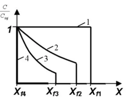
Figure 4 – Concentration waves for different particle sizes. Each front moves with velocityα(rs). Line 1 corresponds to transport of small particles (rs1 <rpmi n). Lines 2 and 3 are related to filtration of intermediate size particles,rs2 <rs3. Line 4 shows
the large particle concentration (rs4>rpmax).
Figure 5 – Concentration distributions for suspended particles and vacant pores during filtration: (a) initial distributions; (b) distributions behind the concentration front for
Figure 6 – Suspended concentration at the core outlet. Lines 1 and 3 are related to large and small particles, respectively. Line 2 corresponds to intermediate size particle
concentration.
Figure 7 – Effect of particle size on dimensionless penetration depthhX(r s)imax for
intermediate size particles. Three curves were calculated for three different pore size distributions assuming the same average pore size(hr pi =11µm), standard deviation
Figure 8 – Shapes of suspended particle and vacant pore size distributions. Areasc1and
c3represent the fraction of particles that do not perform deep bed filtration (small and