www.scielo.br/cam
On a continuum theory of brittle materials
with microstructure
FERNANDO PEREIRA DUDA1
and ANGELA CRISTINA CARDOSO DE SOUZA2
1Programa de Engenharia Mecânica, COPPE/UFRJ, Cx. Postal 68503 21945-970 Rio de Janeiro, Brasil
2Laboratório de Mecânica Teórica e Aplicada, PGMEC/TEM/UFF Rua Passo da Pátria 156, sala 409 – 24210-240 Niterói, Brasil
E-mails: [email protected] / [email protected]
Abstract. This paper deals with a finite strain continuum theory of elastic-brittle solids with microstructure. A single scalar microstructural field is introduced, meant to represent – even if in a summary way – the concentration of microdefects within the material. A system of micro-forces, dual to the microstructural field, is axiomatically introduced. The corresponding balance, augmented with suitable constitutive information, yields,inter alia, a kinetic equation for the mi-crostructural field, criteria for damage nucleation, growth and healing as well as a failure criterion based on attainment of a critical value of the microstructural field. The theory is applied for the description of the Mullins effect.
Mathematical subject classification: 74C15, 74C20.
Key words:continuum mechanics, damage mechanics, brittle materials.
1 Introduction
There are many circumstances where the macroscopic behavior of solids is strongly influenced by processes on the microscale. This is the case, for in-stance, of the dynamic fracture behavior of brittle solids, where the macroscopic behavior is governed by nucleation, growth and coalescence of microcracks (see Ravi-Chandar, 1998).
In this paper we deal with the development of a finite strain continuum theory for the behavior of elastic-brittle solids that accounts for: microscale processes, by introducing a scalar microstructural field and the corresponding microforce system; rate and nonlocal effects, by including constitutive dependences on the rate and the gradient of the microstructural field. The microstructural field may represent, for instance, the cohesion state within the material: it varies from 1 (pristine material) to 0 (cracked-up material).
The main ingredients of our theory are the following: i) basic laws: the standard force and moment balances; the microforce balance; the dissipation inequality that includes, via the microforces, the power expended during microstructural changes, ii) constitutive theory: constitutive equations consistent with the dis-sipation inequality, that include both rate and gradient dependence on the mi-crostructural field. The basic laws are postulated following the framework de-veloped by Fried and Gurtin (1994) and Gurtin (1996). The microforce balance, augmented with suitable constitutive information, yields: a kinetic equation for the microstructural field; criteria for both cohesion decreasing (damage initia-tion and growth) and cohesion increasing (damage healing); the noinitia-tion of elastic range; a failure criterion based on the attainment of a critical value of the mi-crostructural field; a criterion for damage healing impossibility. Also, the model can describe distinct behavior under traction and compression.
An application of the presented theory for the description of the stress-softening phenomenon, also called the Mullins effect, is outlined. This phenomenon is typical for many materials such as rubbers, elastomers and biomaterials (see, for instance, Krishnaswamy and Beatty (2000), Beatty and Krishnaswamy (2000), DeSimoneet al(2001) and references cited therein.).
The present modelling approach is similar to the dynamic fracture modelling approaches presented by Aransonet al (2000) and Karmaet al(2001). But in contradistinction to their work, our approach is based on a clear separation of basic balance laws from constitutive equations, including dissipation. In this respect, our theory is similar to the isotropic damage theory presented by Costa-Mattos and Sampaio (1995), and Frémond and Nedjar (1996).
constitutive theory is presented in Section 3, where constitutive assumptions are introduced and restricted by using the Coleman-Noll (1963) principle. Section 4 presents the theory for the case in which the microstructural field is the cohesion descriptor. Application for the description of the Mullins effect is outlined in Section 5.
We adopt notations commonly used in continuum mechanics (see Gurtin, 1981). Symbols and quantities are defined when they first appear.
2 Basic notions
LetBbe a body identified with the bounded region of space it occupies in a fixed
reference configuration. The macrokinematics is described by the motiony,
y:(X, t )→x, (1)
which maps the particle located atX∈ Bat timetto its placexand is
one-to-one at eacht, with deformation gradientF := ∇yconsistent with detF > 0. The microkinematics is described by the macroscopic scalar field α, with gradient:
p:= ∇α, (2)
so that α(X, t ) characterizes the observed microstructure at the particle X at timet.
We characterize the standard force system by the first Piola-Kirchhoff stressS
and by body force per unit volume1b, both measured in the reference configu-ration. Then, the standard force and moment balances are, respectively,
∂P
SndA+
P
bdV=0,
∂P
(y−y0)×SndA+
P
(y−y0)×bdV=0,
(3)
wherePis an arbitrary part ofB,nthe unitary exterior normal to the boundary of P(∂P),y0is an arbitrary spatial point anda×crepresents the vectorial product
of the vectorsaandc. In local form, the standard force and moment balances are respectively:
DivS+b=0,
SFT =FST, (4)
where DivAdenotes the divergence of the tensor or vector fieldA.
The working of the standard forces on a part P is defined by the classical
relation:
Ws(P)=
∂P
Sn· ˙ydA+
P
b· ˙ydV=
P
S· ˙FdV, (5)
whereA·B=tr(ATB), forAandBtensors, anda·cis the usual internal product for the vectorsaandc. The last equality is obtained by using(4)1.
The microforce system is characterized by the microstress vectorξ, the (scalar) internal microforceπ, the (scalar) external microforceµ. The microforce system is constrained by the microforce balance:
∂P
ξ·ndA+
P
(µ−π )dV=0, (6)
which in local form is:
Divξ −π+µ=0. (7)
The working of the microforces on a partPis given by:
Wm(P)=
∂P
(ξ·n)α˙ dA+
P
µα˙dV=
P
(ξ· ˙p+πα)˙ dV, (8)
where the last equality is obtained by using (7).
Within the present purely mechanical context, the Second Law, or Dissipation Inequality, takes the form:
˙
P
ψdV
≤Ws(P)+Wm(P), for each partP, (9)
whereψis the free energy per unit referential volume. The corresponding local form is given by:
˙
3 Constitutive theory
We consider constitutive equations givingψ,S,ξ andπ at any given point and time when:
(σ,α)˙ :=(F, α,p,α)˙ (11)
are known at that point and time; i.e.,
ψ = ˆψ (σ,α),˙ S= ˆS(σ,α),˙ ξ = ˆξ (σ,α),˙ π = ˆπ (σ,α).˙ (12)
We assume that: ψˆ,Sˆ andξˆare smooth functions;πˆ is smooth whenα˙ =0 with jump discontinuity atα˙ = 0. Thus,π is constitutively determined only when
˙
α=0. Otherwise, it is constitutively indeterminate and defined by (7).
By inserting (12) into the dissipation inequality (10) we obtain the functional inequality:
(∂Fψˆ − ˆS)· ˙F+(∂pψˆ − ˆξ )· ˙p+(∂αψˆ − ˆπ )α˙ +∂α˙ψˆ α¨ ≤0. (13)
Following the Coleman-Noll procedure we conclude that:
(i) the response functionψˆ does not depend onα˙, i.e,
∂α˙ψˆ =0; (14)
(ii) the response functionψˆ andSˆ must be related through.
ˆ
S=∂Fψˆ; (15)
(iii) the response functionsψˆ andξˆ must be related through
ˆ
ξ =∂pψˆ; (16)
(iv) the response functionsπˆ must comply with the residual inequality
ˆ
which implies that2:
⎧
⎨
⎩ ˆ
πd ≥0 if α >˙ 0,
ˆ
πd ≤0 if α <˙ 0.
(18)
It is convenient to use the additive decomposition ofπˆd:
ˆ
πd = ˆπdri+ ˆπ rd
d , (19)
into rate-independent (πˆdri) and rate-dependent (πˆdrd ) parts, where:
⎧
⎪ ⎨
⎪ ⎩
ˆ
πdri(σ ):=A+(σ ), πˆdrd(σ,α)˙ :=B+(σ,α)˙ if α >˙ 0,
ˆ πri
d (σ ):=A−(σ ), πˆdrd(σ,α)˙ :=B−(σ,α)˙ if α <˙ 0,
A±(σ ):=lim
ǫ→0πˆd(σ,±ǫ),
B±(σ,α)˙ := ˆπd(σ,α)˙ −A±(σ ),
(20)
and, in order to satisfy (18), we assume in what follows that:
A+≥0, A−≤0, B+≥0 and B−≤0. (21)
Using the results obtained so far and assuming that µ = 0, we write the microforce balance (7) as:
⎧
⎨
⎩
Div∂pψ (σ )ˆ − ˆπ (σ,α)˙ =0 if α˙ =0,
π =Div∂pψ (σ )ˆ if α˙ =0,
(22)
whereπˆ is given by
ˆ
π (σ,α)˙ := ˆπd(σ,α)˙ +∂αψ (σ ).ˆ (23)
The distinction between (22)1and (22)2is very important: the first is a restriction
on the manner in which microstructural changes may occur; the second is an identity that definesπwhen there are no microstructural changes, which implies that the microforce balance is automatically satisfied.
2We remark that by definition,πˆ
dandπˆ have the same properties as far as their dependence
4 Special theory
We may interpret the microstructural fieldα as the cohesion variable: it varies from 1 (pristine material) to 0 (cracked-up material). In the continuum damage mechanics literature(1−α)is called the damage variable. Ifα >˙ 0 (α <˙ 0) in a given material point, its cohesion is undergoing a positive (negative) growth.
Now, we specialize the theory by assuming that the free energy response is given by:
ˆ
ψ (F, α,p)= ˆφ(F, α)+ ˆf (α)+ ˆg(p), (24)
whereφˆis the strain energy response, which is such thatφ(ˆ F,0)=0,φ(ˆ I, α)=0 and:
τ (F, α):=∂αφ(ˆ F, α) >0 if F=I. (25)
The functionfˆrepresents the cohesion energy response and the gradient energy responsegˆ is assumed to be given by:
ˆ
g(p)= 1 2κ|p|
2, (26)
whereκ ≥0 is a material constant.
As we already remarked, the microforce balance restricts the manner in which microstructural changes occur (α˙ =0). Thus, in the current context, microstruc-tural changes (equation (22)1) are restricted by:
⎧
⎨
⎩
B+(σ,α)˙ =R+(σ,△α)−τ (F, α) if α >˙ 0,
B−(σ,α)˙ =R−(σ,△α)−τ (F, α) if α <˙ 0,
(27)
where:
R±(σ,△α):=κ△α−f′(α)−A±(σ ). (28)
From the above definition and the constitutive assumptions made so far (A+≥0, A− ≤0), we can observe thatR−≥R+.
Equation(27)1implies that:
is a necessary condition for positive cohesion growth, whereas equation(27)2
implies that:
τ (F, α) > R−(σ,△α) (30)
is a necessary condition for negative cohesion growth.
It is somewhat illuminating to interpret the first term of right hand side of (28). It measures the difference between the cohesion variable at a point and its mean value at neighboring points. It is positive (negative) if this difference is negative (positive).
4.1 Kinetic equation and elastic range
Now, we assume that both (29) and (30) are also sufficient conditions for mi-crostructural changes. Thus,
R+≤τ ≤R− ⇔ α˙ =0. (31)
Therefore, from (27), we write the kinetic law forαas:
⎧
⎪ ⎪ ⎪ ⎪ ⎪ ⎨
⎪ ⎪ ⎪ ⎪ ⎪ ⎩
B+(σ,α)˙ =R+(σ,△α)−τ (F, α) if τ (F, α) < R+(σ,△α),
˙
α=0 if R+(σ,△α)≤τ (F, α)≤R−(σ,△α),
B−(σ,α)˙ =R−(σ,△α)−τ (F, α) if τ (F, α) > R−(σ,△α).
(32)
Equations(32)1and(32)3correspond to positive(α >˙ 0)and negative(α <˙ 0)
cohesion growth, respectively. Equation(32)2corresponds to situations where
the cohesion state is frozen in. In this case, no microstructural changes occur and the material behaves elastically. Thus, we define the Elastic RangeEas the
set of all F, for a fixed (α,p,△α), such that:
R+(F, α,p,△α) < τ (F, α) < R−(F, α,p,△α). (33)
4.2 Damage healing and irreversibility
already discussed, a necessary and sufficient condition for damage healing is given by(29):
τ (F, α) < R+(σ,△α), (34)
where we may interpret
R+(σ,△α)=κ△α−f′(α)−A+(σ ) (35)
as the damage healing driving force.
We see that both first and second terms of the right hand side of the above equation favour damage healing only when: △α > 0, which means that in comparison with the point in question the cohesion of neighboring points are higher; f′(α) < 0, which means that, from the energetic point of view, the material point prefers the virgin state. On the other hand, the third term never favours damage healing becauseA+ ≥ 0. Also, from (25), we see thatτ ≥ 0 always opposes damage healing.
Let us assume that, for a fixed(F,p,△α),R+is a nondecreasing function of α. In this case, the conditionR+<0 means that damage healing is impossible even ifτ =0. Also, let us write the condition (34) in terms ofα. For this, we first define for a fixed(F,p,△α), the critical value ofα–αH – as the solution, if it
exists, of the equationR+(F, αH,p,△α)=0. Then, we conclude that damage
healing is impossible wheneverα < αH.
4.3 Damage nucleation, growth and failure criterion
As we already discussed, a necessary and sufficient condition for negative cohe-sion growth is given by(30):
τ (F, α) > R−(σ,△α), (36)
where we interpret:
R−(σ,△α)=κ△α−f′(α)−A−(σ ) (37)
△α >0, which means that in comparison with the point in question the cohesion of neighboring points are higher;f′(α) <0, which means, from the energetic point of view, that the material point prefers the virgin state. Also, the third term always opposes damage growth becauseA− ≤ 0. Also, from (25), we see that τ ≥0 drives the decohesion process.
Let us assume that, for a fixed(F,p,△α),R−is a nondecreasing function ofα. This means that, in a given material point, the resistance can not decrease if the cohesion increases. In this case, we discuss a special case under which negative cohesion growth is always possible. This case is given by the conditionR− <0, which means that damage grows without resistance even if τ = 0. For this reason, we interpret this condition as a failure criterion. It is convenient to write the condition (36) in terms ofα. For this, we first define for a fixed(F,p,△α), the critical value ofα–αC– as the solution, if it exists, of the equation
R−(F, αC,p,△α)=0.
Therefore, we conclude that damage grows without resistance wheneverα < αC.
It is convenient to split the negative cohesion growth into damage nucleation and damage growth. By damage nucleation we mean a negative cohesion growth in the special case where, at a point,α =1,△α=0 andp=0. Otherwise, we have damage growth. Thus, damage nucleation takes place whenever:
τ (F,1) > Y1:= −f′(1)−A−(F,1,0),
whereY1is the damage nucleation threshold. On the other hand, damage growth
takes place whenever:
τ (F, α) > Y2:=κ△α−f′(α)−A−(σ ),
whereY2is the damage growth threshold.
Finally, we remark that the damage resistance functionR−is analogous to the
R-curvein fracture mechanics. Its dependence onFallows the damage resistance
5 Example: Mullins effect
As an application of the modelling framework developed in this paper, we present in this section some qualitative results related to the stress-softening phenomenon (Mullins effect) as is outlined by Krishnaswamy and Beatty (2000).
We consider an uniaxial extension described by:
x1=λX1, x2=δX2, x3=δX3, (38)
wherexi andXI are the cartesian coordinates ofxandX(equation (1)), andλ
andδare positive constants.
The principal invariants of the right Cauchy-Green strain tensorC=FTFare:
I1=trC=λ2+2δ2,
I2=
1 2
I12−tr(C2) =2λ2δ2+δ4, I3=detC=λ2δ4.
(39)
To model certain foamed rubbers Krishnaswamy and Beatty (2000) use the following strain energy function for the pristine material:
˜
W (I1, I2, I3)=
µ0
2
I2
I3 +
2I3−5
, (40)
whereµ0 is a positive material constant. By assuming that the strain energy
response is
ˆ
φ(F, α)=αW (ˆ F)=αW (¯ C)=αW (I˜ 1, I2, I3), (41)
it follows from equation (25) that
τ = µ0 2
4√λ+λ−2−5, (42)
and, by equation (15), that the components of first Piola-Kirchhoff stressS, which is given by
areSij =0 fori=j, and
S11=
αµ0
λδ2
λδ4−
δ λ
2
, S22=S33=
αµ0
δ3 (λδ 4
−1).
In the case of an uniaxial stress state, whereS11 = SandS22 = S33 = 0, we
have that
δ=λ−1/4,
S=αµ0λ−1/2(1−λ−5/2),
(44)
whereas the corresponding component of the Cauchy stress is
T11 =T =αµ0(1−λ−5/2). (45)
We also assume that gradient effects are negligible, which means thatκ :=0 in equation (26), and that the cohesion energy (24) is given by:
f (α):= 1
b(αlnα−α), (46)
whereb >0 is a material parameter. We choose a simple constitutive function forB+andB−in equation (20):
B+(σ,α)˙ :=B−(σ,α)˙ :=βα,˙ (47)
where β > 0 is the kinetic modulus. We also choose in equation (20) the following constitutive functions:
A−(σ ):= ⎧
⎨
⎩
aT if λ >1,
aC if 0< λ≤1,
A+(σ ):=c α,
(48)
where, by (21), c≥0, aT ≤0 andaC ≤0. Notice that, as we already remarked,
Taking into account the aforementioned constitutive assumptions, the equation (32) is now written as:
⎧
⎪ ⎪ ⎪ ⎨
⎪ ⎪ ⎪ ⎩
βα˙ =R+−τ if τ < R+,
˙
α =0 if R+ ≤τ ≤R−,
βα˙ =R−−τ if τ > R−,
(49)
where:
τ = µ0 2
4√λ+λ−2−5,
R+ = −lnα b −c α,
R− = ⎧
⎪ ⎪ ⎨
⎪ ⎪ ⎩
−lnα
b −aC if 0< λ≤1,
−lnα
b −aT if λ >1.
(50)
Equation (49), which is a rate-dependent kinetic law for α, is similar to the viscoplastic regularization of the Perzyna type (see Simo and Hughes (1999)), in which the rate-independent law is recovered by takingβ →0.
Let us define the normalized quantities:
H∗= H µ0
where H =T , S, τ, β, c, aT, aC and b∗=b µ0.
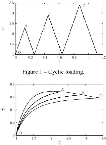
We consider initially the cyclic loading shown in Figure 1. Figure 2 shows the normalized Cauchy stressT∗versus the stretchλwith the parameters:
b∗=0.4, aT∗ =aC∗ =0, c∗=105
(which means that there is not damage healing) and β∗ = 0.005 s−1 (which
means that this case is rate-independent). Observe that this curve is very close to the one obtained by Krishnaswamy and Beatty (2000).
It is interesting to observe the same situation in a rate-dependent model, by using β∗=0.5 s−1. Figure 3 shows the response for this case.
1 1.5 2 2.5 3 3.5
0 0.2 0.4 0.6 0.8 1 1.2
λ
t
O A
B
C
Figure 1 – Cyclic loading.
0 0.2 0.4 0.6 0.8
1 1.5 2 2.5 3 3.5
T∗
λ
O
A
B C
Figure 2 – Rate-independent response.
0 0.2 0.4 0.6 0.8 1
1 1.5 2 2.5 3 3.5
T∗
λ
O
A
B C
Figure 3 – Rate-dependent response.
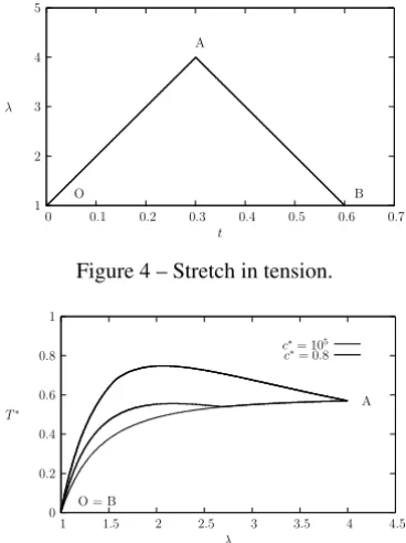
Figure 5 shows the normalized Cauchy stressT∗versus the stretchλwith the parameters: b∗ =0.4, aT∗ =aC∗ =0, c∗ =105(without damage healing) and
1 2 3 4 5
0 0.1 0.2 0.3 0.4 0.5 0.6 0.7
λ
t O
A
B
Figure 4 – Stretch in tension.
0 0.2 0.4 0.6 0.8 1
1 1.5 2 2.5 3 3.5 4 4.5
T∗
λ
O = B
A
c∗= 105
c∗= 0.8
Figure 5 – Damage healing in Cauchy stress×stretch curve.
0.5 0.6 0.7 0.8 0.9 1 1.1
1 1.5 2 2.5 3 3.5 4 4.5
α
λ O
A B
B
c∗= 105
c∗= 0.8
Figure 6 – Damage healing in damage variable×stretch curve.
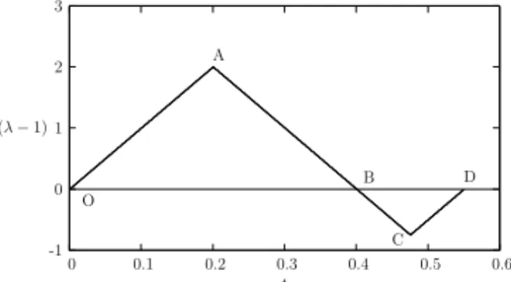
We show in Figure 8 different tensile and compressive responses under the loading history shown in Figure 7. In this case we use the following parameters:
b∗=0.4, a∗T = −0.1, a∗C= −1.0, c∗=10
5
-1 0 1 2 3
0 0.1 0.2 0.3 0.4 0.5 0.6 (λ−1)
t
O
A
B
C D
Figure 7 – Tensile and compressive stretch.
-8 -6 -4 -2 0 2
-1 -0.5 0 0.5 1 1.5 2 2.5
T∗
(λ
−1)
O = B
A
C
Figure 8 – Different tensile and compressive responses.
6 Conclusions
We have proposed a finite strain continuum theory to describe the behavior of elastic-brittle solids with microstructure. The microstructure was described by a single scalar microstructural field. A system of microforces, dual to the mi-crostructural field, was axiomatically introduced. The corresponding balance, augmented with suitable constitutive information, yielded a kinetic equation for the microstructural field, criteria for damage nucleation, growth and healing as well as a failure criterion based on attainment of a critical value of the mi-crostructural field. The potentiality of the theory was addressed by applying it to the description of the Mullins effect.
Acknowledgements
REFERENCES
[1] I.S. Aranson, V.A. Kalatsky and V.M. Vinokur, Continuum Field Description of Crack Prop-agation,Phys. Rev. Lett.85 (2000), 118–121.
[2] M.F. Beatty and S. Krishnaswamy, The Mullins effect in equibiaxial deformation,J. Appl. Math. Phys.(ZAMP),51(2000), 984–1015.
[3] B.D. Coleman and W. Noll, The thermodynamics of elastic materials with heat conduction and viscosity,Arch. Rational Mech. and Analysis,13(1963), 167–178.
[4] H. Costa Mattos and R. Sampaio, Analysis of the fracture of brittle elastic materials using a continuum damage model,Structural Eng. Mech.3(1995), 411–427.
[5] A. DeSimone, J.J. Marigo and L. Teresi, A damage mechanics approach to stress softening and its application to rubber,Eur. J. Mech. A/Solids,20(2001), 873–892.
[6] M. Frémond and B. Nedjar, Damange, gradient of damage and principles of virtual power, Int. J. Solids Structures,33(8) (1996), 1083–1103.
[7] E. Fried and M.E. Gurtin, Dynamic solid-solid transition with phase characterized by an order parameter,Physica D,72(1994), 287–308.
[8] M.E. Gurtin, Generalized Ginzburg-Landau and Cahn-Hilliard equations based on a micro-force balance,Physica D,92(1996), 178–192.
[9] M.E. Gurtin, An Introduction to Continuum Mechanics, Academic Press, New York (1981). [10] A. Karma, D.A. Kessler and H. Levine, Phase-field model of mode III dynamic fracture,
Phys. Rev. Lett.87(4) (2001), 455011-455014.
[11] S. Krishnaswamy and M.F. Beatty, The Mullins effect in compressible solids,Int. J. Eng. Sci.38(2000), 1397–1414.
[12] K. Ravi-Chandar, Dynamic fracture of nominally brittle materials,Int. J. Fracture,90(1998), 83–102.
[13] J.C. Simo and T.J.R. Hughes, Computational Inelasticity, Springer Verlag, Berlin (1999). [14] S.R. White, N.R. Sottos, P.H. Geubelle, J.S. Moore, M.R. Kester, S.R. Sriram, E.N.