www.scielo.br/cam
Homogenisation of magneto-elastic behaviour:
from the grain to the macro scale
LAURENT DANIEL*, OLIVIER HUBERT and RENÉ BILLARDON
LMT-Cachan, ENS Cachan, CNRS (UMR 8535), Université Paris 6 61 avenue du Président Wilson – 94235 CACHAN Cedex – France
E-mail: [email protected]
Abstract. The prediction of the reversible evolution of macroscopic magnetostriction strain and magnetisation in ferromagnetic materials is still an open issue. Progress has been recently made in the description of the magneto-elastic behaviour of single crystals.
Herein, we propose to extend this procedure to the prediction of the behaviour of textured soft magnetic polycrystals. This extension implies a magneto-mechanical homogenisation. The model proposed is discussed and the results are compared to experimental data obtained on industrial iron-silicon alloys.
Mathematical subject classification: 74F15, 74Q05, 74Q15, 74M05, 78M40. Key words: multiscale approach, homogenisation, magnetoelastic couplings, magnetostriction strain, polycrystals.
1 Introduction
The prediction of the magnetic behaviour of ferromagnetic materials, even in the isotropic case is still an active field of research (Bozorth, 1951; Jiles, 1991; A. Hubert et al., 1998). Another open issue is the prediction of the strain in-duced by magnetisation, called magnetostriction, which is closely linked to the magnetisation process, and to the magnetic domains structure. The mechanisms involved in this process can be naturally written at the magnetic domain scale – that is lower than the grain size – whereas the scale of interest for electrical
#575/03. Received: 15/IV/03. Accepted: 02/X/04.
engineering – the machine scale – is nearest to the centimeter scale. The object of this paper is to propose a multi-scale approach that could link these two different scales, providing a macroscopic magneto-elastic model with a strong physical content.
After an illustration of some magneto-elastic effects, a brief description of the magnetisation process is given. A micromagnetic model for single crystals, proposed by Buiron et al. (1999, 2001) is presented as well as its extension to polycrystalline media. The results are then compared to experimental data and discussed.
2 Magneto-elastic couplings
Magnetic and mechanical behaviours are coupled. It means that the magnetic behaviour cannot be accurately determined unless the mechanical fields are taken into account, and, on the other hand, the deformation state is depending on the magnetic configuration. This coupling has two main consequences.
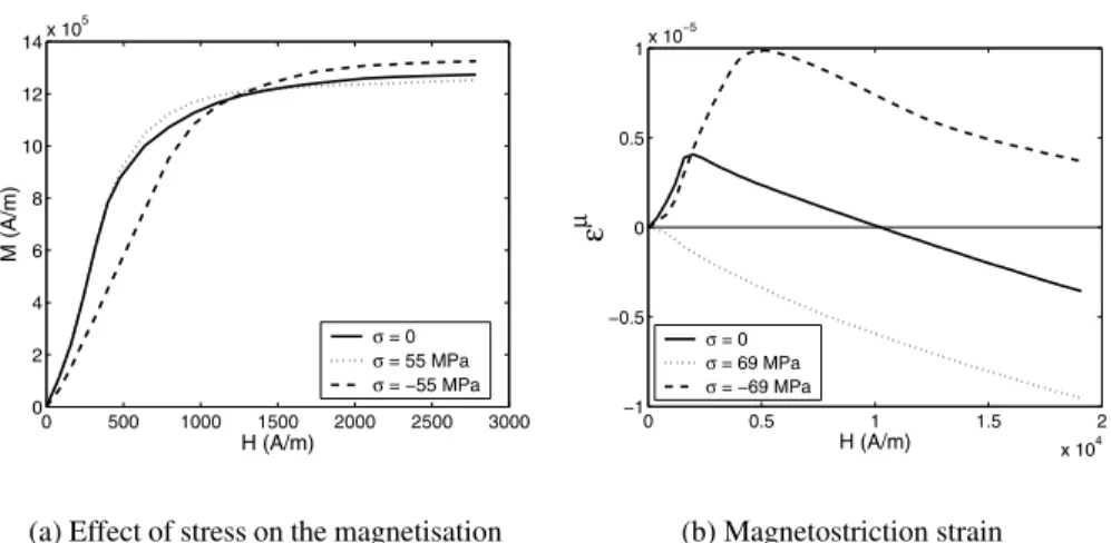
2.1 Stress effect on magnetisation
In the case of Nickel, a compressive stress of 70 MPa doubles the initial per-meability while the same amount of tensile stress reduces it about one tenth of the zero stress value. On the contrary, for materials like 68-permalloy (68% Ni-Fe alloy), the effect of stress is just the opposite. The magnetic behaviour of polycristalline iron under stress is much more complicated. At low magnetic fields, tension raises the M-H curve whereas it lowers it for higher magnetic fields (Villari effect – see for example Cullity (1972)).
2.2 Magnetostriction strain
0 500 1000 1500 2000 2500 3000 0
2 4 6 8 10 12 14x 10
5
H (A/m)
M (A/m)
σ = 0
σ = 55 MPa
σ = −55 MPa
(a) Effect of stress on the magnetisation curve
0 0.5 1 1.5 2
x 104 −1
−0.5 0 0.5
1x 10 −5
H (A/m)
ε
µ
σ = 0
σ = 69 MPa
σ = −69 MPa
(b) Magnetostriction strain
Figure 1 – Experimental llustration of magneto-elastic couplings in iron, after
Cul-lity (1972).
Moreover, this phenomenon explains several particular behaviours, such as the Eeffect or the INVAR and ELINVAR effects (Bozorth, 1951).
TheEeffect is an apparent loss of linearity in the elastic behaviour of demag-netised specimens. This is due to the superimposition of the magnetostriction strain to the elastic strain during the strain measurement (see figure 2). Linear be-haviour is recovered when the stress is high enough to saturate magnetostriction.
σ
ε
εµ sat
saturated
demagnetised
Figure 2 – Illustration ofEeffect.
thermal dilatation in a specific range of temperature, due to the superimposition of the magnetostriction strain to the thermal strain. The ELINVAR effect is the apparent constancy of the Young modulus with a change in temperature.
These complex coupling phenomena are supposed to be strongly correlated with the magnetic microstructure, and thus have to be described and modelled at the relevant scale. This point is the object of next section, where the study has been restricted to polycristalline media, and where the case of iron-based alloys is emphasized.
3 Magnetisation process at the grain scale
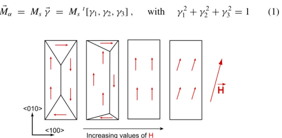
Each grain of a ferromagnetic polycrystalline material is divided into domains (figure 3) that are magnetised at saturation, whatever the external magnetic field (Bozorth, 1951). In each domainα, the magnetisationMα can be written:
Mα = Ms γ = Ms t[γ1, γ2, γ3], with γ12+γ 2 2 +γ
2
3 =1 (1)
Increasing values of H
H
<100> <010>
Figure 3 – Magnetisation process – Schematic two-dimensionnal representation in the case of iron crystal.
rotates towards the direction of the magnetic field. When complete magnetic sat-uration is reached, each grain is composed of a unique domain that is magnetised in the direction of the applied field.
4 Microscopic model
The first step of this magneto-mechanical modelisation is to get an accurate description of the single crystal behaviour, accounting for the two distinct mech-anisms involved in the magnetisation process. It can be noticed that the same model can be applied for a grain embedded in a polycrystal.
4.1 Magnetostriction strain
If the magnetisationMα is known, the magnetostriction strainε µ
αin the domain
is known and can be written in the crystallographic frame CF. In the case of a cubic crystallographic symmetry, the tensorεµα is (A. Hubert et al., 1998):
εµα =
3 2
λ100γ12−1 3
λ111γ1γ2 λ111γ1γ3
λ111γ1γ2 λ100
γ2 2 −
1 3
λ111γ2γ3
λ111γ1γ3 λ111γ2γ3 λ100γ32−1 3
CF
(2)
whereλ100andλ111are the magnetostrictive constants for the single crystal,λ100 (resp. λ111) being the strain measured in the direction parallel to the<100> (resp. <111>) axis of a single crystal, when it is magnetised at saturation along this axis.
Relation (2) can be written in the following condensed form:
εµα =D :γ (3)
defining:
γ = γ⊗ γ
D = 3
2
λ100Ka+λ111Kb
with1:
Ka = L−J
Kb = I−L
Lij kl = δijδklδik
Jij kl = 13δijδkl
(5)
4.2 Mechanical behaviour
Considering the low level of stresses that will be considered hereafter, the me-chanical behaviour of a single crystal is written in the framework of linear elas-ticity, with an usual Hooke law:
σg =CI : εeg (6)
where σg andεeg denote the stress and the elastic strain tensors in the single
crystal whereas CI is the stiffness tensor for the single crystal, assumed to be magnetic field independent.
4.3 Magnetic behaviour
We use here after the description of the magneto-elastic behaviour of single crystals proposed by Buiron et al. (1999, 2001). This approach is derived from Néel magnetic phase model (Néel, 1944).
4.3.1 Magnetic state variables
The state variables chosen to describe the magnetisation of a single crystal are divided in two distinct sets. For each domain familyα, we define:
• The disorientation angleθα being the angle between the crystallographic
easy direction of the α domain family and the present direction of its magnetisationMα. We assume here thatMαis always in the plane formed
by the easy direction and the magnetic field.
• The volumetric fractionfα of theα domain family in the single crystal.
1δ
4.3.2 Potential energy of a domain
In order to determine the state variables, we write the potential energy at the magnetic domain scale, considering three major contributions:
Wα =Wαmag+W an
α +W
σ
α (7)
• Wmag
α is the magnetostatic energy, tending to create a magnetisation
par-allel to the magnetic field. It can be written:
Wαmag= −µ0Hg· Mα (8)
whereHgdenotes the mean magnetic field in the crystal andMα the
mag-netisation in theαdomain:Mα = Msγ = Ms t[γ1, γ2, γ3].
• Wan
α is the anisotropy energy tending to prevent, in each domain, the
rotation of the magnetisation from the easy axes. In the case of cubic crystallographic structure:
Wαan =K1
γ12γ 2 2 +γ
2 2γ
2 3 +γ
2 3γ
2 1
+K2γ12γ 2 2γ
2 3
(9)
whereK1andK2denote the anisotropy constants for the single crystal.
If we note:
β =Kb:γ , (10)
the anisotropy energy can be written:
Wαan =
K1
2 β:β+K2.det(γ −β) (11)
• Wσ
α is the magneto-elastic energy describing the couplings effects between
the magnetisation and the local stressσg (mean value within the single
crystal):
Wασ = −σg : εαµ= −σg : D : γ (12)
whereεµαis the magnetostriction strain tensor in theαdomain, defined by
Using the previous notations, the total potential energy of a domain is defined by equation (13):
Wα = −µ0Hg.Mα+
K1
2 β:β+K2.det(γ −β)−σg:D:γ (13)
This expression does not account for the exchange energy and for the pure elastic energy. The elastic energy is assumed to be constant over a grain, and thus does not participate to the equilibrium of a single crystal. On the other hand, the variations of the exchange energy near the domains border is accounted for thanks to the parameterAs presented here after (Buiron, 2000).
4.3.3 State variables calculation
• Theθαvariables are obtained after minimisation of the potential energy of
each domain family:
Wα(θα)=min(Wα) , θα ∈ [0, θmax] (14)
Ifu0 is the initial easy axis for the domainα,θmaxis defined by:
θmax = Arccos
u0· Hg || Hg||
(15)
• The fα variables are obtained using the explicit relation proposed by
Buiron et al. (2001):
fα =
exp(−As ·Wα)
6
α=1
exp(−As ·Wα)
(16)
whereAs is an adjustment parameter, accounting for the non uniformity
4.3.4 Definition of the single crystal behaviour
Once the state variables are known for each domain familyα, we can define the magnetisation as the mean magnetisation over the crystal:
Mg = Mα =
6
α=1
fαMα (17)
We can also define the mean magnetostriction strain in the single crystal:
εµg = εµα =
6
α=1
fαεµα (18)
4.4 Results
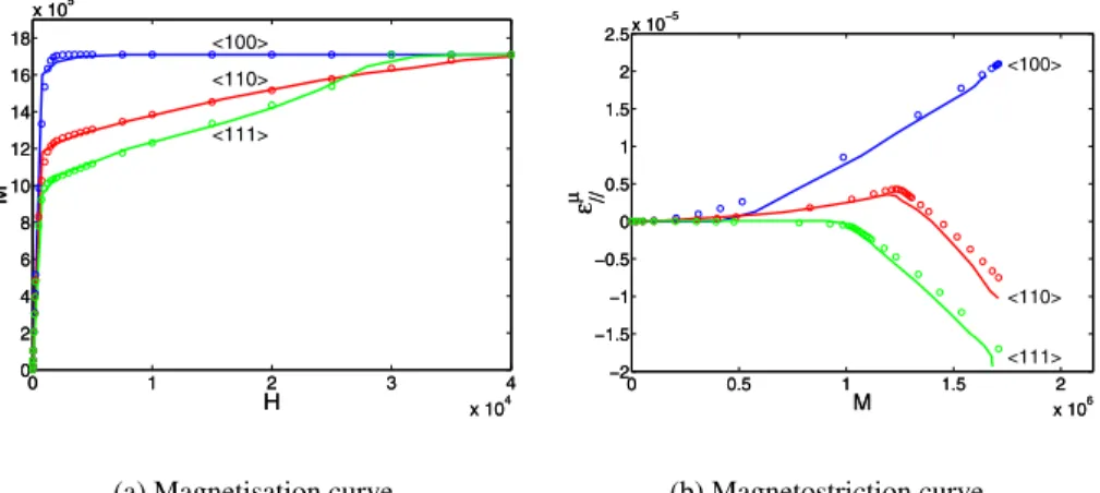
Experimental measurements are available in the litterature for pure iron single crystal2(Webster, 1925). The material constants used are as follows:
C11I =238 GPa; C12I =142 GPa;
C44I =232 GPa.(McClintock et al., 1966) Ms =1,71.106A/m.(Bozorth, 1951)
λ100=2,1.10−5; λ111 = −1,7.10−5.(Bozorth, 1951) K1=42,7 kJ/m3;K2=0.(Bozorth, 1951)
(19)
Figure 4 shows a very good agreement between experimental and numerical results, both concerning the magnetisation and the magnetostriction.
5 Multiscale model
In the case of polycrystalline media, the strain, the stress, the magnetisation and the magnetic field are not homogeneous within the material. The local behaviour (at the grain scale) has to be written with respect to the local loading. This local loading can be, with specific assumptions concerning the microstructure, deduced from the macroscopic loading.
0 1 2 3 4 x 10⁴ 0 2 4 6 8 10 12 14 16 18
x 105
H
M
<100>
<110>
<111>
0 1 2 3 4
x 104 0 2 4 6 8 10 12 14 16 18
x 105
H
M
<100>
<110>
<111>
(a) Magnetisation curve
0 0.5 1 1.5 2
x 106 −2 −1.5 −1 −0.5 0 0.5 1 1.5 2 2.5x 10
−5 M ε // µ <100> <110> <111>
0 0.5 1 1.5 2
x 106 −2 −1.5 −1 −0.5 0 0.5 1 1.5 2 2.5x 10
−5 M ε // µ <100> <110> <111>
(b) Magnetostriction curve
Figure 4 – Iron single crystal anhysteretic behaviour – Experimental (Webster, 1925)
(lines) and modelled (points) data.
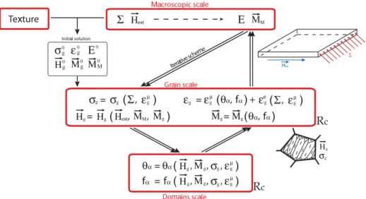
5.1 Multiscale approach – principle
We work on a Representative Volume Element (RVE) of a polycrystalline ferro-magnetic material. Its texture is known through an Orientation Data File obtained after an EBSD (or X-ray) measurement. The single crystal properties (detailed in equation (19)) are known.
The objective is to link the macroscopic response (mean magnetisationMM
and strainE) of this RVE to the macroscopic loading (the external fieldHextand
the macroscopic stress).
The general idea of this micro-macro approach (see figure 5) is to postulate a localisation law, in order to calculate the local loading. The micro-model is then applied at the domains scale and the macro-level is reached through an averaging operation. Since both the local values for the stress and the magnetic field depend on the local magnetisation and strain, an iterative process has to be used.
Iterativ e scheme Hext Σ Texture Rc Rc Macroscopic scale
Σ Ηext Ε ΜΜ
σg Ηg
Domains scale
θα θα Ηg Μg σg εg
µ
= ( , , , )
fα fα Ηg Μg σg εg
µ
= ( , , , )
Grain scale
Σ σg σg εg
µ
= ( , )
Ηg=Ηg(Ηext,ΜΜ,Μg) Μg=Μg(θα,fα)
εg εg
µ
θα fα εg
e = ( , )+ Initial solution σg 0 Ηg 0 εg 0 Μg 0 Ε0 ΜM 0
Σ εg
µ
( , )
Figure 5 – Multi-scale scheme.
5.2 Localisation step
5.2.1 Elastic behaviour
The aim of this step consists in deriving the local stress from the external loading, postulating a particular form for the functiongin relation (20).
σg =g
, Hext
(20)
The functiong is here deduced from a self-consistent approach. Each grain is considered as an inclusion in the homogeneous medium equivalent to the polycrystal, so that the problem can be linked to the solution of the Eshelby inclusion problem (Esheby, 1957).
The magnetostriction strain εµg is considered as a free strain. The Eshelby
tensorSE is calculated3following Mura (1982).SE links the free strain (εµ g) in
a region (the inclusion) of the infinite media to the total strainεI in this region:
εI =SE :εµg (21)
From the Eshelby solution, we can deduce, through a self-consistent scheme, the stiffness tensor of the homogeneous medium equivalent to the polycrystal. Details of this approach are given in appendix A. Each grain (of stiffness CI) is considered as an inclusion in this equivalent homogeneous medium. The equivalent stiffness tensorCeffis solution of the implicit equation (22):
Ceff = CI :(CI +C∗)−1:(Ceff+C∗) (22)
where the symbol < . >denotes an averaging operation over the volume and
C∗denotes the Hill constraint tensor.
We can also define the two 4t h order localisation operators (see details in
appendix A):
• the strain localisation tensorA:
A=(CI +C∗)−1:(Ceff+C∗) (23)
• the stress concentration tensorB:
B=CI :A:Ceff−1 (24)
This scheme is used to express the relation (20). The local stress is written as the sum of two terms (equation (25)).
σg =B: +CI :
SE−I
:εµg (25)
The first one depends on the macroscopic stress tensor and on the stress concentration law. The second term is linked to the elastic incompatibility strain due to the existence of a free strainεµg in the grain, and to the stiffness of the
surrounding medium. In the case of iron-silicon alloys, the magnetostriction magnitude – that do not exceed 10−5 – justify the fact that the incompatibility stresses involved remain in the elastic domain.
It must be noticed that this relation is an implicit relation, sinceεµg is a function
5.2.2 Magnetic behaviour
The aim of this step consists in deriving the local magnetic field from the external loading, postulating a given form for the functionhin relation (26).
Hg =h
, Hext
(26)
This equation is usually written (in electrotechnical engineering) in the form of relation (27).
Hg = Hext+ Hd (27)
where the local perturbation of the macroscopic magnetic field is taken into account through the demagnetising fieldHd. The general form of the localisation
law can be written:
Hg− Hext =K(MM− Mg) (28)
withMM the mean magnetisation in the material,Mg the local magnetisation.
K is a 2nd order operator, depending on the magnetisation, on the stress state, and on the shape choosen for the inclusion.
In the case of stress independent linear isotropic magnetic behaviour, and spherical inclusions, the tensor K can be replaced by a scalar value Nc (see
appendix B).
Nc=
1 3+2χM
, χM being the equivalent media susceptibility (29)
Herein, as a first approximation, we choose to extend this relation to anisotropic non-linear magnetic behaviour. We keep the form of equation (28), and use a particular value forNc. It could also be possible to use a variable value ofNc
computed from the value ofχM recalculated at each step of the iterative scheme.
5.3 Local behaviour
The grain behaviour model has been described in paragraph 4. From the local loadingσg andHg, we can obtain in each grain the magnetisationMg and the
5.4 Homogenisation
The last step in the micro-macro modelisation is the homogenisation step to get back to the macro-scale. We define:
MM = <Mg >
E = <εg >
(30)
As the scheme is self-consistent, an iterative procedure has to be built up. The calculation is then done until convergence.
6 Results and comparison to experimental data
100 mµ
(a) Optical observation (b) EBSD texture measurement
Figure 6 – Observation of a commercial Fe-3%Si alloy.
Computations have been made using a 500 grains RVE of an industrial alloy. This commercial iron-silicon alloy indicates no morphologic texture (figure 6(a)). The mean grain size is about 70µm. The texture is known thanks to EBSD measurements (figure 6(b)).
strong influence on the magneto-mechanical behaviour). The specimens are cut every 10◦from the rolling direction (RD).
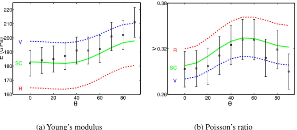
6.1 Macroscopic elastic behaviour
Tensile tests have been carried out to measure the Young’s modulus and the Poisson’s ratio thanks to standard strain gauges measurements. Young’s modulus and Poisson’s ratio evolution in the sheet plane are plotted in figure 7(a) and 7(b). A good agreement between experimental and numerical data is shown. Calculations using the Reuss and Voigt extremal hypotheses are also plotted.
0 20 40 60 80
160 170 180 190 200 210 220
θ
E (G
Pa) V
R
SC
(a) Young’s modulus
0 20 40 60 80
0.26 0.32 0.38
θ
ν
V
R
SC
(b) Poisson’s ratio
Figure 7 – Experimental () and modelled elastic properties evolution, with respect to the orientation in the sheet plane. Symbols SC, V and R respectively refer to the
self-consistent, Voigt and Reuss hypotheses.
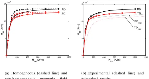
6.2 Macroscopic magnetic behaviour
Two kinds of calculations have been made concerning the magnetic uncoupled behaviour: firstly without considering any demagnetising field (homogeneous magnetic field hypotheses: Nc = 0, Hg = Hext), and secondly introducing a
demagnetising field calculation (Nc=5.10−4).
It must be noticed that the resolution of the implicit equation (28) leads, in the case of non-linear behaviour to numerical difficulties: the computational costs are high, and the convergence depends on the quality of the initial solution in the general algorithm (see figure 5): an appropriate choice of this initial solution enables to avoid dissuasive computation times.
Magnetic measurements were obtained using a non-standard experimental frame (Hubert et al., 2002). The results are plotted on figure 8(b).
0 200 400 600 800 1000 1200
0 5 10 15x 10
5
H
ext (A/m) MM
(A/m)
RD T D
(a) Homogeneous (dashed line) and non-homogeneous magnetic field calculations.
0 200 400 600 800 1000 1200
0 5 10 15x 10
5
H
ext (A/m) MM
(A/m)
RD T D
RD
exp
T Dexp
(b) Experimental (dashed line) and numerical results.
Figure 8 – Experimental and numerical anhysteretic magnetisation curves in the rolling
(RD) and in the transverse direction (TD).
60 80 100 120 140 0
10 20 30 40 50 60 70 80 90 100
460 480 500 520 540
0 10 20 30 40 50 60 70 80 90 100
960 980 1000 1020 1040
0 10 20 30 40 50 60 70 80 90 100
H (A/m) H (A/m)
H (A/m)
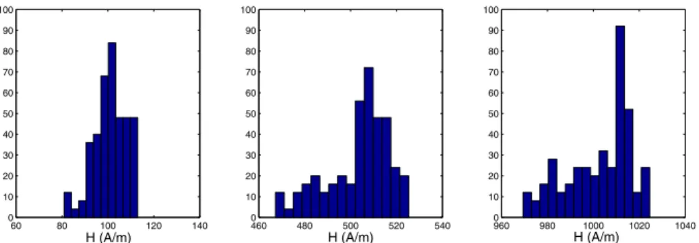
Figure 9 – Local magnetic field heterogeneity for|| Hext||= 100, 500 and 1000 A/m
within a VER constituted of 500 grains.
Comparison with experimental data (figure 8(b)) shows a good qualitative agreement, although the predicted magnetisation is over-estimated.
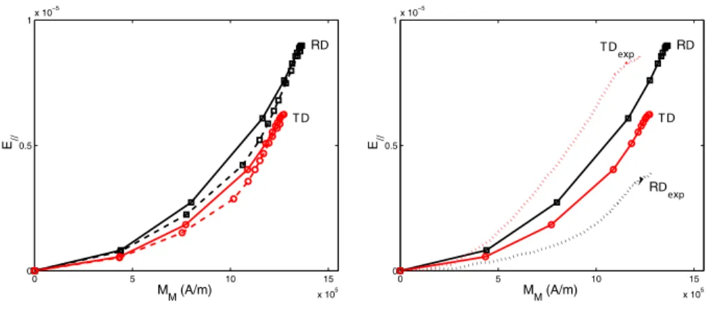
6.3 Macroscopic magnetostrictive behaviour
The same experimental procedure, with strain gauges, is used to measure mag-netic strains. These mesurements are corrected to deduct the so-called form-effect (Billardon et al., 1995; Daniel et al., 2003) and obtain the true magne-tostriction strain. Experimental and numerical results are plotted on figure 10.
The demagnetising field calculation tends to weakly reduce the magnetostric-tion amplitude (figure 10(a)). The predicted general level is correct compared to experimental measurements (figure 10(b)), but the relative anisotropy between the rolling and the transverse directions is not respected. This problem is the object of a work in progress (Daniel et al., 2003); this point is related to the initial state of the specimens, and particularly residual stresses and surface ef-fects, that can explain this disagreement beetween calculation and experimental observations (Daniel, 2003).
7 Conclusion
0 5 10 15 x 105 0
0.5 1x 10
−5
MM (A/m)
T D RD
E//
(a) Homogeneous (dashed line) and non-homogeneous magnetic field cal-culations.
0 5 10 15
x 105 0
0.5 1x 10
−5
MM (A/m)
T D RD
E//
RDexp T Dexp
(b) Experimental (dashed line) and nu-merical results.
Figure 10 – Experimental and numerical anhysteretic magnetostriction curves in the rolling (RD) and in the transverse direction (TD).
materials. The level of magnetostriction can also be predicted.
Several works are presently in progress to improve this micro-macro approach. A first way is to refine the magnetic localisation law, for example introducing a magnetic field dependency forKin equation (28).
Another direction would be to get a more precise description and understand-ing of the domains microstructure. This description is presently limited to the volumetric fractionfαand the disorientation angleθα for each domain family.
This kind of micro-macro strategy could then participate in the understanding of the effect of stress on the magnetic behaviour, especially in the case of multi-axial loadings.
I I I
ε
Lε
IC
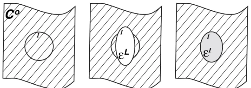
oFigure 11 – Schematic representation of the Eshelby’s inclusion problem.
Consider an unloaded homogeneous infinite medium of moduliCo. A regionI
of this medium (the inclusion) is submitted to a free strain εL. This strain is the strain that would act in the inclusion if no resistance was exerted by the surrounding medium. The actual strainεI in the inclusion can be linked to the free strain using the Eshelby tensor (Esheby, 1957):
εI =SE :εL (31)
The fourth order tensor SE only depends on the elastic moduli Co and on
the shape chosen for the inclusion. Elements concerning the calculation of this tensor can be found in Mura (1982). The stress in the inclusion is linked to the elastic strain by the Hooke relation:
σg =Co :εeg =Co :
εI −εL=Co :
SE−I:εL (32)
It can be shown (Bornert et al., 2001) that the problem of an elastic heterogene-ity (that is the case considered for polycrystals) can be reduced to an inclusion problem. A fictive equivalent free strainεL∗is defined, that would lead to the same strain and stress state in the inclusion than the one acting in the hetero-geneity. The macroscopic loading is defined by the macroscopic stress, and the macroscopic strain is E. Stress and strain in the inclusion are defined by relations (33) and (34)
σg =+Co :
SE−I:εL∗ (33)
that can be written:
εL∗ =SE−1 :
εI −E (35)
Introducing this relation in equation (33), one obtains:
σg =+C∗:E−εI (36)
C∗being the Hill constraint tensor defined by relation (37):
C∗=Co :(SE−1−I) (37)
If we now come back to the problem of the elastic heterogeneity (the strain being purely elastic), the behaviour law is:
σg =CI :εeg =CI :εI (38)
and at the macroscopic scale:
=Ceff :E (39)
From equation (36), it comes:
CI :εI =Ceff :E+C∗ :
E−εI
(40)
that leads to:
εI =
CI +C∗−1:Ceff +C∗:E (41)
that can also be written using equation (38):
σg =CI :
CI +C∗−1
:
Ceff+C∗
:E (42)
The strain localisation tensor is derived from equation (41):
A=(CI+C∗)−1:(Ceff+C∗) (43)
This fourth order operator links the macroscopic strain to the local strain in the inclusion:
The stress concentration tensor is derived from equation (38), (39) and (44):
B=CI :A:Ceff−1 (45)
This fourth order operator links the macroscopic stress to the local stress in the inclusion:
σg =B: (46)
The definitions ofAandBare given in the paper as equation (23) and (24). The macroscopic stress is linked to the local stresses through relation (47) (equation (42) is used):
= σg
= CI :
CI+C∗−1
:
Ceff+C∗
:E
= CI :
CI+C∗−1
:
Ceff+C∗
:E
(47)
This leads to a relationship that must be verified by the effective moduli tensor
Ceff, noted equation (22) in the paper:
Ceff= CI :(CI +C∗)−1:(Ceff+C∗) (48)
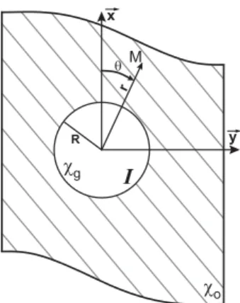
Appendix B: Determination of the magnetic field localisation operator Relations (28) and (29) defining the localisation law for the magnetic field are derived from the solution of a magnetostatic problem for an inclusion.
We consider a spherical isotropic magnetic region embedded in an infinite isotropic magnetic medium. This medium is submitted to an uniform (at the boundary) magnetic fieldH∞ =H∞x.
The behaviour law for the spherical region (of radius R) is written:
Mg =χgHg (49)
The behaviour law for the infinite medium is written:
Fo
R r x
y
M
T
I
Fg
Figure 12 – Schematic representation of the inclusion problem.
Without any current density, the Maxwell equations can be written:
divB =0, whereBdenotes the magnetic induction,
rotH = 0, whereH denotes the magnetic field. (51)
Under these conditions, the magnetic field can be derived from a scalar poten-tial:
H = − gradϕ (52)
Applying the isotropic behaviour law (B =µH) leads to the Poisson equation for the potential:
ϕ =0 (53)
The solutions for the potentialϕcan be written:
ϕg = −Hgrcosθ, inside the sphere
ϕo = −H∞r
1− k
r3
cosθ , outside the sphere (54)
H∞ being the value for the magnetic field very far from the inclusion. The magnetic field can then be written, following equation (52):
– inside the sphere:
– outside the sphere:
Ho=H∞ 1+
k r3(3 cos
2θ−1)
x+3k
r3 cosθsinθ y
(56)
The boundary conditions at the interface of the inclusion give (n is the unit vector normal to the sphere surface):
a) forθ = π
2 andr =R:
[ H] ∧ n=0 ⇒ Hg =H∞
1− k
R3
(57)
where the symbol [ H] denotes the jump of H through the surface ([ H] =
Hext− Hint).
From equation (57) we can deduce:
k=
1− Hg
H∞
R3 (58)
b) forθ =0 andr =R:
[ B].n = [ H + M].x=0 ⇒ Mg+Hg =Mo(0, R)+Ho(0, R)
⇒ Mg+Hg =(χo+1) H∞
1+ 2k
R3
(59)
Replacing the value ofkin equation (59) leads to:
Mg+Hg =(χo+1) H∞
3−2Hg
H∞
(60)
that can also be written:
Mg+3Hg+2χoHg=2χoH∞+M∞+3H∞ (61)
finally leading to the expression:
Hg−H∞=
1 3+2χo
As both magnetisation and magnetic fields appearing in equation (62) are parallel to the directionx, this relation can be written in a vectorial way:
Hg− H∞=
1 3+2χo
(M∞ − Mg) (63)
This relation justify the choice made for relation (28), and the particular value ofNcin equation (29).
REFERENCES
[1] Billardon R. and Hirsinger L.,J. Mag. Mag. Mat.,140-144(1995), 2199.
[2] Bornert M., Bretheau T. and Gilormini P., Homogénéisation en mécanique des matériaux. Tome 1: Matériaux aléatoires élastiques et milieux périodiques, Hermès Science Paris (2001).
[3] Bozorth R.M., Ferromagnetism, Van Nostrand New York (1951).
[4] Buiron N., Modélisation multi-échelle du comportement magnéto-élastique couplé des matéri-aux ferromagnétiques doux, Thèse de doctorat, Ecole Normale Supérieure de Cachan, France (2000).
[5] Buiron N., Hirsinger L. and Billardon R.,J. Phys. IV,9(1999), 187–196.
[6] Buiron N., Hirsinger L. and Billardon R.,J. Phys. IV,11(2001), 373–380.
[7] Cullity B.D., Introduction to magnetic materials, Addison-Wesley (1972).
[8] Daniel L., Modélisation multi-échelle du comportement magnéto-mécanique des matériaux ferromagnétiques texturés, Thèse de doctorat, Ecole Normale Supérieure de Cachan, France (2003).
[9] Daniel L., Hubert O., Ossart F. and Billardon R.,J. Phys. IV,105(2003), 247–253.
[10] Eshelby J.D.,Proc. R. Soc. Lond.,A421(1957), 376.
[11] Hubert A. and Schäfer R., Magnetic domains, Springer (1998).
[12] Hubert O., Influence des contraintes internes et de la structure des dislocations sur les couplages magnéto-mécaniques dans les alliages Fe-3%Si à grains non orientés, Thèse de doctorat, Université Technologique de Compiègne, France (1998).
[13] Hubert O., Daniel L. and Billardon R.,J. Mag. Mag. Mat.,254-255C(2002), 352–354.
[14] Jiles D.C., Introduction to Magnetism and Magnetic Materials, Chapman and Hall (1991).
[15] McClintock F.A. and Argon A.S., Mechanical behavior of materials, Addison-Wesley Pub-lishing Company (1966).
[16] Mura T., Micromechanics of defects in solids Martinus Nijhoff Publishers (1982).
[17] Néel L.,J. Phys. Radiat.,5(1944), 241.