Carry trade returns and foreign exchange rate risk

(1)

1

A Work Project, presented as part of the requirements for the Award of an International Master Degree in Finance from the NOVA – School of Business and Economics and INSPER.

CARRY TRADE RETURNS AND FOREIGN EXCHANGE RATE RISK

EMERSON MARQUES DA SILVA - 3129

A Project carried out on the International Master in Finance Program at Nova School of Business & Economics, under the supervision of Professor Dr. André Silva, and on the Master in

Economics and Finance at INSPER under supervision of Professor. Dr. Marco Lyrio

(2)

2

Carry Trade Returns and Foreign Exchange Rate Risk

Abstract

This paper analyses whether foreign exchange risk measures and its components have the ability to predict the return to the carry trade strategy. We employ a dynamic portfolio composed of 20 currencies. We first show that carry trade returns are related to the total variance of our portfolio of currencies. We then decompose the total variance of this portfolio in a component representing the average variance of this portfolio and another representing its average correlation. Since average correlation is not significantly related to carry trade returns, the predictive power of market variance is primarily attributable to average variance.

Keywords: carry trade, average variance, average correlation, quantile regression.

1. Introduction

The carry trade is a currency trading strategy that recommends borrowing in low-interest currencies and investing in high-interest currencies. This strategy exploits deviations from the Uncovered Interest Rate Parity (UIP). UIP implies that the expected carry trade return should be equal to zero. This is the case since the interest rate differential would on average be offset by a depreciation of the investment currency. There are a number of empirical evidences pointing to the rejection of the UIP (e.g., Bilson, 1981; Fama, 1984). If this is indeed the case, investors can expect to make a profit with the carry trade strategy since it is expected that the investing currency will depreciate less that what is predicted by the UIP. Since we assume that Covered Interest Rate Parity (CIP) holds, this empirical evidence is called the forward premium puzzle.

(3)

3

The natural interpretation for a high average payoff to the carry trade strategy is that it compensates agents for bearing risk. The analysis of the intertemporal tradeoff between currency risk and carry trade return has four objectives. The first objective is to evaluate if current portfolio volatility can predict future carry trade return. The second objective is to assess the predictive ability of exchange rate risk on the distribution of carry trade returns using quantile regressions. The changes in exchange rate risk are related to gains or losses with carry trade that are in the right tail or left tail of the return distribution, respectively. The third objective is to define a group of currency risk measures that explains the movements in aggregate volatility and correlation. The forth objective is to evaluate the economic gains of the analysis through a version of carry trade strategy that is conditioned by risk measures. This paper analyses these points for different portfolios.

2. Theoretical Motivation

Merton (1973, 1980) suggests that there is a linear relation between the expected excess return of a risky market portfolio and the conditional market variance. According to Merton (1973, 1980), risk-averse investors require a higher risk premium to hold aggregate wealth as systematic risk increases, so the expected return must rise. The empirical evidence of the sign and statistical significance of the intertemporal risk-return tradeoff in equity markets is inconclusive. This relation has been found insignificant and sometimes even negative (e.g., French et al., 1987; Goyal and Santa Clara, 2003). The Intertemporal Capital Asset Pricing Model (ICAPM) can be applied to the currency market as any risky asset in any market. Thus, the intertemporal risk return tradeoff of the carry trade can be expressed by:

(4)

4

where rC,t+1 is the portfolio excess return of the carry trade from time t to t+1; MVt is the

conditional variance of the currency portfolio return at time t, denominated FX portfolio variance; and εt+1 is the normally distributed error term at time t+1.

Equation (1) indicates a linear relation between the FX portfolio variance and future excess returns. The coefficient k represents the investors’ risk aversion and the natural interpretation is that is positive, that is, as the risk increases, the risk-averse investor requires a higher risk premium and higher expected return.

Pollet and Wilson (2010) show that the variance can be decomposed in average variance and average correlation for equity returns. This decomposition is critical for determining whether the potential predictive ability of the market variance is due to movements in average variance or average correlation. Thus, the variance decomposition can be expressed by:

𝑀𝑉_𝑡 = 𝜑₀+ 𝜑₁𝐴𝑉_𝑡+ 𝜑₂𝐴𝐶_𝑡 , (2)

where MVt is the conditional variance of the currency portfolio return at time t, denominated FX

portfolio variance; AVt is the equally weighted cross-sectional average of the variances of all

exchange rate excess returns at time t; ACt is the equally weighted cross-sectional average of the

correlation of each pair of all exchange rate excess returns at time t.

Equation (2) indicates a linear relation between FX portfolio variance and average variance and average correlation. Pollet and Wilson (2010) show that this relation is positive for average variance and average correlation (ϕ1,ϕ2 > 0). Thus, we have the following hypothesis.

Hypothesis 1: The FX portfolio variance is a predictor of future FX excess returns due to two components: average variance and average correlation.

(5)

5

Furthermore, this paper analyses if there is an intertemporal risk-return tradeoff of carry trade by quantile of the distribution. The functions conditioned to quantile τ implied by equations (1) and (2) are defined as:

𝑄_𝑟_𝐶,𝑡+1(𝜏 | 𝑀𝑉𝑡) = 𝜇 + (𝑘 + 𝑄𝜏𝑁) + (𝑘 + 𝑄𝜏𝑁) 𝑀𝑉𝑡

= 𝛼(𝜏) + 𝛽(𝜏) 𝑀𝑉_𝑡 , (3)

𝑄𝑟𝐶,𝑡+1(𝜏 | 𝐴𝑉𝑡, 𝐴𝐶𝑡) = 𝜇 + 𝜑0(𝑘 + 𝑄𝜏𝑁) + (𝑘 + 𝑄𝜏𝑁)𝜑1𝐴𝑉𝑡+ (𝑘 + 𝑄𝜏𝑁)𝜑2𝐴𝐶𝑡

= 𝛼(𝜏) + 𝛽₁(𝜏)𝐴𝑉𝑡+ 𝛽2(𝜏)𝐴𝐶𝑡 , (4)

where QτN is the τ-th quantile of the distribution, which has a large negative value deep in the left

tail and a large positive value deep in the right tail. As k>0 and ϕ1,ϕ2 > 0, it is expected that the risk measures have negative coefficients in the left tail and positive coefficients in the right tail.

In high volatility periods, the shocks (resulting in losses) are amplified when investors hit cash constraints and unwind their positions, which further depress prices and increase the cash problems and volatility. According to Cenedese, Sarno and Tsiakas (2014) this asymmetric effect indicates that volatility is negatively related to carry trade returns and high volatility has more effect on the left tail of the distribution of returns. Thus, we have the following hypothesis.

Hypothesis 2: The predictive power of risk measures (FX portfolio variance, average variance and average correlation) varies between quantile of the distribution of FX excess returns, and is strongly negative in the lower quantile.

(6)

6

3. Data sets

All currencies are quoted in amounts of domestic currency (US dollar) per unit of foreign currency. We use two data sets: one including spot exchange rates and the other forward exchange rates. The period of the data sets is from Feb-1999 to Jul-2016 and the data sets were collected from Bloomberg. The first data set includes 20 countries in advanced and emerging market economies. The second data set is formed by the 10 developed economies of the total data set: Australia, Canada, Denmark, Euro area, Japan, New Zealand, Norway, Sweden, Switzerland and United Kingdom. The third data set contains the remaining 10 emerging market economies: Brazil, Colombia, Czech Republic, Mexico, Philippines, Poland, Singapore, South Africa, Taiwan and Thailand. The first 3 years of the data set were used to make the first set to augmented strategies. So, the statistics and graphics comparing standard carry trade with augmented carry trade strategies start in Feb-2002.

4. Methodology

a) Carry trade for individual currencies

The carry trade strategy for individual currencies can be implemented in two ways. In the first, the investor takes a long position in a forward contract today in order to exchange the domestic currency into foreign currency in the future. The payoff of the forward contract can be converted into the domestic currency at the future spot exchange rate. The excess return to this strategy is

defined as: 𝑟_𝑗,𝑡+1 = 𝑠_𝑗,𝑡+1− 𝑓_𝑗,𝑡 (5)

for j={1,2,...,N} where N is the number of currencies at time t; rj,t+1 is the excess return of

currency j for one-period; sj,t+1 is the log of the nominal spot exchange rate defined as the

(7)

7

rate j at time t, which is the rate established in the contract at time t for an exchange of currencies at t+1. A depreciation of the domestic currency (US dollar) is an increase in sj,t+1.

In the second form of the carry trade strategy, the investor buys a foreign bond and sells a domestic bond at the same time. Both bonds are risk free in their currencies but the investor is exposed to FX risk in the foreign bond. The excess return to this strategy is defined as:

𝑟_𝑗,𝑡+1= 𝑖_𝑗,𝑡∗ _{− 𝑖}

𝑡+ 𝑠𝑗,𝑡+1− 𝑠𝑗,𝑡 , (6)

where it and ij,t* are the one-period domestic and foreign nominal interest rates, respectively.

According to the Covered Interest Rate Parity (CIP), in the absence of arbitrage, the following condition must apply:

𝑓_𝑗,𝑡− 𝑠_𝑗,𝑡 = 𝑖_𝑡− 𝑖_𝑗,𝑡∗ _. ₍₇₎

If UIP holds, on average, the excess return on the two forms will be equal to zero, so the carry trade strategy is not profitable. That is, the interest rate differential is on average offset by a depreciation of the invested currency. So, the forward premium (fj,t – sj,t) should be equal to the

interest rate differential.

b) Portfolio of Currencies

All currencies are sorted according to the forward premium value (fj,t – sj,t) at the beginning of each month. IF CIP holds, the currencies are sorted from low to high forward premium, which is equivalent to sort from the low to high interest rate differential. The sample is divided into 5 portfolios (quintiles) each month. Portfolio 1 is the portfolio with the highest interest rate currencies and portfolio 5 is the portfolio with the lowest interest rate currencies. The carry trade

(8)

8

portfolio goes long on portfolio 1 and short on portfolio 5. The carry trade portfolio monthly return from time t to t+1 is defined as rC,t+1.

c) FX Portfolio Variance

The excess return to the FX portfolio is the equally weighted excess return of all currencies of

the data set. 𝑟_𝑃,𝑡+1= 1

𝑁𝑡∑ 𝑟𝑗,𝑡+1

𝑁𝑡

𝑗=1 . (8)

The monthly MV is estimated using daily excess returns according to the following equation:

𝑀𝑉_𝑡+1 = ∑𝐷𝑡 𝑟_{𝑃,𝑡+𝑑/𝐷}2 _𝑡

𝑑=1 + 2 ∑ 𝑟𝑃,𝑡+𝑑/𝐷𝑡

𝐷𝑡

𝑑=2 𝑟𝑃,𝑡+(𝑑−1)/𝐷𝑡, (9)

where Dt is the number of trading days in month t, typically Dt = 21. The sample mean is not

subtracted from each daily return in calculating the variance because this adjustment is very small (Merton, 1980).

d) Average Variance and Average Correlation

The general formula of portfolio variance is:

𝜎𝑝2 = ∑𝑖=1𝑛 ∑𝑛𝑗=1𝑤𝑖𝑤𝑗𝐶𝑜𝑣(𝑟𝑖, 𝑟𝑗) . (10)

Considering the naive diversification strategy in which an equally weighted portfolio is constructed, meaning that wi = 1/n. We break out the terms for which i=j into a separate sum and

we consider that Cov(ri,ri)=σi2, so the eq. 10 may be rewritten as follows:

𝜎_𝑝2 ₌1 𝑛∑ 1 𝑛𝜎𝑖 2₊ 𝑛 𝑖=𝑗 ∑ ∑𝑛𝑖=1_𝑛12𝐶𝑜𝑣(𝑟𝑖, 𝑟𝑗) 𝑛 𝑗=1 𝑗≠𝑖 . (11)

(9)

9

Note that there are n variance terms and n*(n-1) covariance terms. If we define the average variance as

𝜎2 = 1_𝑛∑𝑛 𝜎_𝑖2

𝑖=1 , (12)

and average covariance as

𝐶𝑜𝑣 = _{𝑛(𝑛−1)}1 ∑𝑛𝑗=1∑𝑛𝑖=1𝐶𝑜𝑣(𝑟𝑖, 𝑟𝑗) 𝑗≠𝑖

, (13)

the portfolio variance can be written as

𝜎𝑝2 =_𝑛1𝜎2+𝑛−1_𝑛 𝐶𝑜𝑣 . (14)

The portfolio becomes highly diversified as n increases. The specific risk, represented by the first term in eq. 14 is diversified away as n becomes greater. The second term simply approaches

Cov as n becomes greater. Note that (n-1)/n=1-1/n, which approaches 1 for large n. Thus the

irreducible risk of a diversified portfolio depends on the covariance of the returns, which in turn is a function of the importance of systematic factors in the economy.

To see further the fundamental relationship between systematic risk and security correlations, suppose for simplicity that all securities (currencies) have a common standard deviation, σ, and all pairs of them have a common correlation coefficient, ρ. Then the covariance between all pairs

of securities is given by: 𝐶𝑜𝑣 = 𝜌 ∗ 𝜎2 . (15)

So the eq. 14 becomes: 𝜎𝑝2 =_𝑛1𝜎2+𝑛−1_𝑛 𝜌𝜎2 . (16)

(10)

10

Note that σp2 = MV, ρ = AC and σ2 = AV. According to Pollet and Wilson (2010), MV is

decomposed in cross-sectional average variance (AV) and cross-sectional average correlation (AC). So, MV is defined as:

𝑀𝑉𝑡+1 = 𝐴𝑉𝑡+1∗ 𝐴𝐶𝑡+1 . (18)

If all exchange rates had equal individual variances, the decomposition above would be exact. The approximation of variance decomposition works very well for a large number of currencies.

The regression of the variance decomposition is defined as:

𝑀𝑉_𝑡+1 = 𝛼 + 𝛽(𝐴𝑉_𝑡+1∗ 𝐴𝐶_𝑡+1) + 𝑢𝑡+1 . (19)

Similarly to Pollet and Wilson (2010), the variance decomposition can be estimated in addition to equation 19, according to the following regressions:

𝑀𝑉_𝑡+1 = 𝛼 + 𝛽𝐴𝑉_𝑡+1+ 𝑢_𝑡+1, (20)

𝑀𝑉𝑡+1 = 𝛼 + 𝛽𝐴𝐶𝑡+1+ 𝑢𝑡+1 , (21)

𝑀𝑉𝑡+1 = 𝛼 + 𝛽1𝐴𝑉𝑡+1+ 𝛽2𝐴𝐶𝑡+1+ 𝑢𝑡+1 . (22)

Just as Cenedese, Sarno and Tsiakas (2014), this paper uses equation 22 to estimate the variance decomposition and to estimate predictive regressions.

The measures of AV and AC are defined as:

𝐴𝑉𝑡+1 = _𝑁1 𝑡 ∑ 𝑉𝑗,𝑡+1 𝑁𝑡 𝑗=1 , (23) 𝐴𝐶𝑡+1 = _𝑁 1 𝑡(𝑁𝑡−1) ∑ ∑ 𝐶𝑖𝑗,𝑡+1 𝑁𝑡 𝑗≠𝑖 𝑁𝑡 𝑖=1 , (24)

(11)

11

where Vj,t+1 is the realized variance of the excess return to currency j at time t+1, and is defined

as: 𝑉𝑗,𝑡+1 = ∑ 𝑟𝑗,𝑡+𝑑/𝐷𝑡 2 𝐷𝑡 𝑑=1 + 2 ∑ 𝑟𝑗,𝑡+𝑑/𝐷𝑡 𝐷𝑡 𝑑=2 𝑟𝑗,𝑡+(𝑑−1)/𝐷𝑡 , (25)

and Cij,t+1 is the realized correlation between the excess returns of currencies i and j at time t+1:

𝐶𝑖𝑗,𝑡+1= _√𝑉 𝑉𝑖𝑗,𝑡+1 𝑖,𝑡+1 √𝑉𝑗,𝑡+1, (26) 𝑉𝑖𝑗,𝑡+1 = ∑ 𝑟𝑖,𝑡+𝑑/𝐷𝑡 𝑟𝑗,𝑡+𝑑/𝐷𝑡 𝐷𝑡 𝑑=1 + 2 ∑ 𝑟𝑖,𝑡+𝑑/𝐷𝑡 𝐷𝑡 𝑑=2 𝑟𝑗,𝑡+(𝑑−1)/𝐷𝑡 . (27) e) Predictive Regressions

Two predictive regressions for one-month horizon are estimated using ordinary least squares (OLS).

The first regression is a way to evaluate the intertemporal risk-return tradeoff in FX. The regression evaluates whether the carry trade has low or negative returns in times of high market variance.

𝑟𝐶,𝑡+1 = 𝛼 + 𝛽𝑀𝑉𝑡+ 𝜀𝑡+1 (28)

The second regression includes the risk-return tradeoff of the variance decomposition proposed by Pollet and Wilson (2010). This regression makes a division between the AV and AC effects with the purpose of evaluating whether these effects bring a more precise signal of future carry trade returns. The constant α is the same for both regressions. Substituting eq. 22 into eq. 28, the regression is defined as:

(12)

12

The first quantile regression (eq. 3) is given by:

𝑄_𝑟_𝐶,𝑡+1(𝜏 | 𝑀𝑉𝑡) = 𝛼(𝜏) + 𝛽(𝜏) 𝑀𝑉𝑡 , (3)

where 𝑄_𝑟_𝐶,𝑡+1(𝜏 | . ) is the τ-th quantile function of one-month ahead carry trade returns conditional on information available at month t.

Substituting eq. 22 into eq. 3, the second quantile regression (eq. 4) is given by:

𝑄_𝑟_𝐶,𝑡+1(𝜏 | 𝐴𝑉_𝑡, 𝐴𝐶_𝑡) = 𝛼(𝜏) + 𝛽₁(𝜏)𝐴𝑉_𝑡+ 𝛽₂(𝜏)𝐴𝐶_𝑡 . (4) 5. Empirical Results

We first present the descriptive statistics of the three data sets used in the analysis: global portfolio, advanced economies and emerging markets. We present the regressions of variance decomposition into AV and AC which will help us to explain the time variation in MV. The OLS regressions of one-month ahead carry trade returns into MV, AV and AC are discussed, as well as the quantile regressions of carry trade returns.

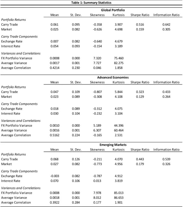
a) Descriptive Statistics

Descriptive statistics on the carry trade strategy (risk and return) for global portfolio, advanced economies and emerging markets are showed in Table 1. The first 3 years of the data set were used to make the first regression of each model. So, the statistics and regressions start in Feb-2002. Considering no transaction costs, the carry trade strategy had an average annualized return of 6.1% (global portfolio), 4.7% (advanced economies) and 6.8% (emerging markets). The annualized standard deviations are 9.5% (global portfolio), 10.9% (advanced economies) and 12.6% (emerging markets).

(13)

13

The interest rate differential is the principal component of the carry trade strategy with average annualized return of 5.4% (global portfolio), 3.0% (advanced economies) and 7.0% (emerging markets). The annualized exchange rate component had an average appreciation of 0.7% (global portfolio), an appreciation of 1.8% (advanced economies) and an average depreciation of 0.3% (emerging markets). These statistics show that exchange rates, on average, only partially offset the interest rate differential. The carry trade strategy has negative skewness and the kurtosis is higher than 3.

The descriptive statistics of the risk measures show that the mean of MV is about half the value of the AV. The mean of AC is 0.42 for global portfolio, 0.52 for advanced economies and 0.39 for emerging markets. MV and AV have high positive skewness and high kurtosis. The global portfolio has higher Sharpe Ratio and Information Ratio in relation to the advanced economies and emerging markets. The graphics of Figure 1 confirm the better performance of the global portfolio in relation to the advanced economies and emerging markets.

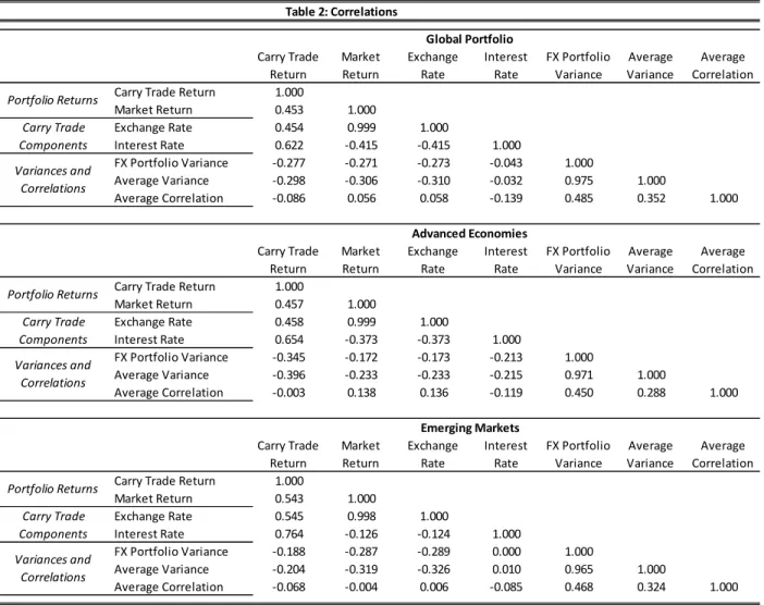
MV and AV are negative correlated with the carry trade and market returns for all three portfolios (Table 2). The correlation between MV and AV is positive and high for global portfolio (0.975), advanced economies (0.971) and emerging markets (0.965). The correlation between AV and AC is positive but moderate. Carry trade and interest rate returns are highly positive correlated for all three portfolios. This correlation is higher than the correlation between carry trade and FX returns for all three portfolios.

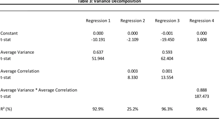
b) Variance Decomposition

The variance decomposition (MV) into AV and AC was described by equation 18. The variance decomposition is evaluated by some regressions that are presented in Table 3. The regression of

(14)

14

MV into product of AV and AC have a slope coefficient of 0.888 and R2 = 99.4%. The regression of MV into AV and AC have slope coefficients of 0.593 and 0.001 respectively and R2 = 96.3%. The analyses of the regressions shows that the AV component are more important to explain the variation in MV, and AV and AC are responsible for almost all of time variation in MV.

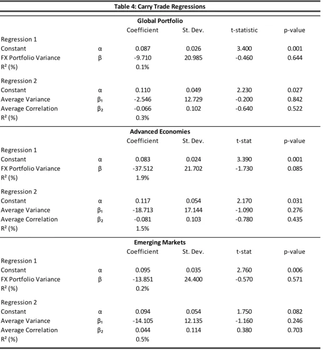
c) OLS Regressions

The OLS regressions of the carry trade strategies are shown in Table 4. The regression of the carry trade returns one-month ahead on MV shows that the relation is negative but not statistically significant for all three portfolios (global portfolio, advanced economies and emerging markets). These results refuse the first hypothesis (H1) that the FX portfolio variance is a predictor of future FX excess returns. There is not significant evidence in the regression of the carry trade return in relation to AV and AC (global portfolio, advanced economies and emerging markets). Thus, MV and its components cannot be used to predict carry trade returns.

d) Quantile Regressions

While OLS regressions analyses the relation between risk and mean returns, the quantile regressions of the carry trade returns one-month ahead on MV analyses the relation by τ-th quantile, as shown in Table 5. There is not significant evidence in the quantile regressions of the future carry trade return in the quantiles of the distribution. The coefficient has more negative values for the lower quantiles but is not statistically significant. These results refuse the second hypothesis (H2) that the predictive power of risk measures varies between quantile of the distribution of FX excess returns, and is strongly negative in the lower quantile.

(15)

15

Table 6 shows the quantile regressions of the carry trade returns one-month ahead on AV and AC. There is not a significant relation for AV and for AC. So, it is not possible to predict carry trade returns using the left tail of the distribution of MV and AV.

6. Augmented Carry Trade Strategies

We develop some augmented carry trade strategies conditioned on market variance. We compare these strategies to the standard carry trade strategy defined in the Portfolio of Currencies session.

a) Trading Strategies

The first carry trade strategy (augmented strategy 1) is conditioned on current market variance (MV). In this strategy, at each month t, if MV from t-1 to t is higher than its median value up to that point, the carry trade positions are closed and the excess return will be zero at t+1, otherwise the standard carry trade strategy is executed.

The second carry trade strategy (augmented strategy 2) is conditioned on left tail of the carry trade returns distribution. In this strategy, at each month t, only for carry trade returns those are lower than τ-quantile of the distribution at month t, if MV from t-1 to t is higher than its median up to that point, the carry trade positions are closed and the excess return will be zero at t+1, otherwise the standard carry trade strategy is executed.

The third carry trade strategy (augmented strategy 3) considers the quantile of returns and do not consider MV. In this strategy, at each month t, if carry trade returns are lower than τ-quantile of the distribution at month t, the carry trade positions are closed and the excess return will be zero at t+1, otherwise the standard carry trade strategy is executed.

(16)

16

These strategies are implemented out of sample. The strategies move forward recursively starting 3 years after the beginning of the sample.

b) The Performance of the Strategies

The augmented strategy 2 is the most important since it considers the left tail of the distribution of carry trade returns and MV. The performance of this strategy can be viewed at Table 7. Relative to the standard carry trade, this strategy has a higher average annualized return (6.70% vs 6.00%), lower annualized standard deviation (8.60% vs 9.50%) and higher Information Ratio (0.780 vs 0.631) for the global portfolio. This strategy has a higher average annualized return (5.60% vs 4.70%), lower annualized standard deviation (9.00% vs 10.90%) and higher Information Ratio (0.626 vs 0.431) for the advanced economies. This strategy has a higher average annualized return (7.70% vs 7.20%), lower annualized standard deviation (11.40% vs 12.50%) and higher Information Ratio (0.672 vs 0.575) for the emerging markets. Figure 2 shows the augmented strategy 2 for all three portfolios.

7. Conclusion

The carry trade strategy tries to exploit deviations from the UIP. The empirical evidence suggests that the interest rate differential across countries is not, on average, offset by the depreciation of the investment currency. So the carry trade strategy has large average returns by borrowing in low-interest currencies and investing in high-interest currencies.

We refuse the hypothesis that FX portfolio variance and its components have a significant effect on the left tail of the distribution of future carry trade returns. Carry trade returns cannot be predicted using market variance and return quantile. Augmented trading strategies combining market variance and return quantile can reduce drawdowns.

(17)

17

Table 1. Descriptive Statistics

The table shows descriptive statistics for the monthly excess returns of three carry trade portfolios: Global Portfolio, Advanced Economies and Emerging Markets. The global portfolio includes 20 exchange rates relative to the US dollar for the sample period of February 2002 to July 2016. The sample period for the Advanced Economies and for Emerging Markets is the same. The mean, standard deviation of returns, Sharpe Ratio and Information Ration are annualized. The Variances and Correlations are for monthly returns. The skewness and kurtosis are for monthly returns.

Table 1: Summary Statistics Global Portfolio

Mean St. Dev. Skewness Kurtosis Sharpe Ratio Information Ratio

Portfolio Returns

Carry Trade 0.061 0.095 -0.358 3.907 0.516 0.642

Market 0.025 0.082 -0.626 4.698 0.159 0.305

Carry Trade Components

Exchange Rate 0.007 0.082 -0.640 4.679

Interest Rate 0.054 0.093 -0.154 3.189

Variances and Correlations

FX Portfolio Variance 0.0008 0.000 7.320 75.460

Average Variance 0.0017 0.001 7.727 82.275

Average Correlation 0.4214 0.230 0.046 1.858

Advanced Economies

Portfolio Returns

Carry Trade 0.047 0.109 -0.807 5.844 0.323 0.433

Market 0.023 0.089 -0.308 4.108 0.129 0.264

Exchange Rate 0.018 0.089 -0.312 4.075

Interest Rate 0.030 0.104 -0.232 3.104

Average Correlation 0.5162 0.224 -0.165 2.531

Emerging Markets

Portfolio Returns

Carry Trade 0.068 0.126 -0.211 4.070 0.443 0.539

Market 0.027 0.082 -0.773 4.956 0.179 0.326

Exchange Rate -0.003 0.082 -0.787 4.912

Interest Rate 0.070 0.106 0.013 3.819

(18)

18

Table 2. Descriptive Statistics

The table shows the correlations for the monthly variables of three carry trade portfolios: Global Portfolio, Advanced Economies and Emerging Markets.

Table 2: Correlations Global Portfolio Carry Trade Return Market Return Exchange Rate Interest Rate FX Portfolio Variance Average Variance Average Correlation

Carry Trade Return 1.000

Market Return 0.453 1.000 Exchange Rate 0.454 0.999 1.000 Interest Rate 0.622 -0.415 -0.415 1.000 FX Portfolio Variance -0.277 -0.271 -0.273 -0.043 1.000 Average Variance -0.298 -0.306 -0.310 -0.032 0.975 1.000 Average Correlation -0.086 0.056 0.058 -0.139 0.485 0.352 1.000 Advanced Economies Carry Trade Return Market Return Exchange Rate Interest Rate FX Portfolio Variance Average Variance Average Correlation

Market Return 0.457 1.000 Exchange Rate 0.458 0.999 1.000 Interest Rate 0.654 -0.373 -0.373 1.000 FX Portfolio Variance -0.345 -0.172 -0.173 -0.213 1.000 Average Variance -0.396 -0.233 -0.233 -0.215 0.971 1.000 Average Correlation -0.003 0.138 0.136 -0.119 0.450 0.288 1.000 Emerging Markets Carry Trade Return Market Return Exchange Rate Interest Rate FX Portfolio Variance Average Variance Average Correlation

Market Return 0.543 1.000 Exchange Rate 0.545 0.998 1.000 Interest Rate 0.764 -0.126 -0.124 1.000 FX Portfolio Variance -0.188 -0.287 -0.289 0.000 1.000 Average Variance -0.204 -0.319 -0.326 0.010 0.965 1.000 Average Correlation -0.068 -0.004 0.006 -0.085 0.468 0.324 1.000 Portfolio Returns Carry Trade Components Variances and Correlations Portfolio Returns Variances and Correlations Carry Trade Components Portfolio Returns Carry Trade Components Variances and Correlations

(19)

19

Table 3. FX Portfolio Variance Decomposition

The table shows the OLS results for regressions on alternative decompositions of the FX portfolio variance. The dependent variable is the FX portfolio variance as defined in this paper. The table shows the regressions of the Global Portfolio, which includes 20 exchange rates relative to the US dollar for the sample period of April 1999 to July 2016. The FX portfolio variance (MV), average variance (AV), average correlation (AC) and the product of average variance * average correlation (AV * AC) are for monthly returns.

The regression 1 is given by: MVt+1 = α + β1(AVt+1) + ut+1.

The regression 2 is given by: MVt+1 = α + β2(ACt+1) + ut+1.

The regression 3 is given by: MVt+1 = α + β1(AVt+1) + β2(ACt+1) + ut+1.

The regression 4 is given by: MVt+1 = α + β(AVt+1 * ACt+1) + ut+1.

Table 3: Variance Decomposition

Regression 1 Regression 2 Regression 3 Regression 4

Constant 0.000 0.000 -0.001 0.000 t-stat -10.191 -2.109 -19.450 3.608 Average Variance 0.637 0.593 t-stat 51.944 62.404 Average Correlation 0.003 0.001 t-stat 8.330 13.554

Average Variance * Average Correlation 0.888

t-stat 187.473

(20)

20

Table 4. OLS Predictive Regressions

The table shows the OLS results for regressions for two predictive regressions. The first regression is: rC,t+1 = α + β MVt + εt+1 as defined by equation 20. The second regression is: rC,t+1

= α + β1 AVt + β2 ACt + εt+1 as defined by equation 21. The table shows the regressions of the

Global Portfolio, which includes 20 exchange rates relative to the US dollar for the sample period of April 1999 to July 2016. The sample period for the Advanced Economies and for Emerging Markets is the same. All variables are annualized, with the exception of average correlation. Newey-West (1987) t-statistics with five lags are reported.

Table 4: Carry Trade Regressions Global Portfolio

Coefficient St. Dev. t-statistic p-value Regression 1 Constant α 0.087 0.026 3.400 0.001 FX Portfolio Variance β -9.710 20.985 -0.460 0.644 R² (%) 0.1% Regression 2 Constant α 0.110 0.049 2.230 0.027 Average Variance β₁ -2.546 12.729 -0.200 0.842 Average Correlation β₂ -0.066 0.102 -0.640 0.522 R² (%) 0.3% Advanced Economies

Coefficient St. Dev. t-stat p-value

Regression 1 Constant α 0.083 0.024 3.390 0.001 FX Portfolio Variance β -37.512 21.702 -1.730 0.085 R² (%) 1.9% Regression 2 Constant α 0.117 0.054 2.170 0.031 Average Variance β₁ -18.713 17.144 -1.090 0.276 Average Correlation β₂ -0.081 0.103 -0.780 0.435 R² (%) 1.5% Emerging Markets

Coefficient St. Dev. t-stat p-value

Regression 1 Constant α 0.095 0.035 2.760 0.006 FX Portfolio Variance β -13.851 24.400 -0.570 0.571 R² (%) 0.2% Regression 2 Constant α 0.094 0.054 1.750 0.082 Average Variance β₁ -14.105 12.135 -1.160 0.246 Average Correlation β₂ 0.044 0.114 0.380 0.703 R² (%) 0.5%

(21)

21

Table 5. Quantile Regressions using FX Portfolio Variance

The table shows the results for quantile regressions for predictive regressions 𝑄𝑟𝐶,𝑡+1(𝜏 | 𝑀𝑉𝑡) = 𝛼(𝜏) + 𝛽(𝜏) 𝑀𝑉_𝑡 as defined by equation 3. The table shows the quantile regressions of the Global Portfolio, which includes 20 exchange rates relative to the US dollar for the sample period of April 1999 to July 2016. The sample period for the Advanced Economies and for Emerging Markets is the same. All variables are annualized, with the exception of average correlation. Bootstrap t-statistics generated using 10,000 bootstrap samples are reported.

Table 5: Quantile Regressions for the Carry Trade Returns Global Portfolio Quantile 0.1 0.2 0.3 0.4 0.5 0.6 0.7 0.8 0.9 Constant Coefficient -0.270 -0.150 -0.077 0.003 0.056 0.156 0.259 0.370 0.474 St. Dev. 0.061 0.036 0.030 0.031 0.029 0.053 0.045 0.046 0.033 t-stat -4.410 -4.190 -2.560 0.100 1.940 2.940 5.760 8.050 14.260 p-value 0.000 0.000 0.011 0.917 0.054 0.004 0.000 0.000 0.000

FX Portfolio Variance Coefficient -67.876 -16.358 -0.330 -5.534 3.669 16.084 3.087 -16.578 9.682

St. Dev. 110.876 58.562 40.363 39.568 42.079 43.708 36.741 44.252 41.482 t-stat -0.610 -0.280 -0.010 -0.140 0.090 0.370 0.080 -0.370 0.230 p-value 0.541 0.780 0.993 0.889 0.931 0.713 0.933 0.708 0.816 R² (%) 2.0% 0.1% 0.0% 0.1% 0.0% 0.2% 0.0% 0.1% 0.2% Advanced Economies Quantile 0.1 0.2 0.3 0.4 0.5 0.6 0.7 0.8 0.9 Constant Coefficient -0.343 -0.122 -0.085 0.016 0.080 0.161 0.256 0.347 0.475 St. Dev. 0.082 0.037 0.046 0.032 0.031 0.044 0.036 0.054 0.047 t-stat -4.190 -3.270 -1.860 0.480 2.530 3.700 7.090 6.420 10.180 p-value 0.000 0.001 0.065 0.629 0.012 0.000 0.000 0.000 0.000

FX Portfolio Variance Coefficient -81.785 -101.544 -23.701 -24.153 -28.740 -34.587 -40.615 -14.600 8.459

St. Dev. 49.994 52.686 52.713 36.476 29.115 29.169 31.656 43.171 59.451 t-stat -1.640 -1.930 -0.450 -0.660 -0.990 -1.190 -1.280 -0.340 0.140 p-value 0.103 0.055 0.653 0.509 0.325 0.237 0.201 0.736 0.887 R² (%) 5.3% 2.8% 1.1% 1.0% 0.6% 0.3% 0.4% 0.2% 0.1% Emerging Markets Quantile 0.1 0.2 0.3 0.4 0.5 0.6 0.7 0.8 0.9 Constant Coefficient -0.433 -0.217 -0.086 0.038 0.123 0.220 0.270 0.421 0.537 St. Dev. 0.040 0.066 0.052 0.037 0.038 0.044 0.037 0.065 0.065 t-stat -10.750 -3.310 -1.660 1.040 3.210 4.990 7.290 6.430 8.220 p-value 0.000 0.001 0.099 0.302 0.002 0.000 0.000 0.000 0.000

FX Portfolio Variance Coefficient -63.401 -8.631 -16.208 -23.406 -21.365 -10.825 2.751 -27.197 104.888

St. Dev. 65.431 66.173 53.160 42.801 39.716 38.526 49.406 78.572 81.893

t-stat -0.970 -0.130 -0.300 -0.550 -0.540 -0.280 0.060 -0.350 1.280

p-value 0.334 0.896 0.761 0.585 0.591 0.779 0.956 0.730 0.202

(22)

22

Table 6. Quantile Regressions using Average Variance and Average Correlation The table shows the results for quantile regressions for predictive regressions 𝑄_𝑟_𝐶,𝑡+1(𝜏 | 𝐴𝑉𝑡, 𝐴𝐶𝑡) = 𝛼(𝜏) + 𝛽1(𝜏)𝐴𝑉𝑡+ 𝛽2(𝜏)𝐴𝐶𝑡 as defined by equation 4. The table shows the quantile regressions of the Global Portfolio, which includes 20 exchange rates relative to the US dollar for the sample period of April 1999 to July 2016. The sample period for the Advanced Economies and for Emerging Markets is the same. All variables are annualized, with the exception of average correlation. Bootstrap t-statistics generated using 10,000 bootstrap samples are reported.

Table 6: Quantile Regressions for the Carry Trade Returns Global Portfolio Quantile 0.1 0.2 0.3 0.4 0.5 0.6 0.7 0.8 0.9 Constant Coefficient -0.173 -0.149 -0.074 0.003 0.049 0.148 0.259 0.421 0.481 St. Dev. 0.097 0.062 0.057 0.054 0.053 0.087 0.074 0.079 0.050 t-stat -1.780 -2.390 -1.290 0.060 0.930 1.700 3.520 5.350 9.680 p-value 0.076 0.018 0.198 0.949 0.353 0.091 0.001 0.000 0.000 Average Variance Coefficient -0.136 0.021 -0.010 0.001 0.058 -0.014 -0.079 -0.201 -0.247 St. Dev. 0.220 0.117 0.116 0.124 0.144 0.213 0.184 0.144 0.140 t-stat -0.620 0.180 -0.080 0.010 0.400 -0.060 -0.430 -1.390 -1.760 p-value 0.538 0.858 0.935 0.993 0.689 0.948 0.670 0.166 0.080 Average Correlation Coefficient -84.392 -13.255 -0.070 -3.538 -7.052 14.432 19.931 21.881 53.685

St. Dev. 68.766 43.224 28.185 28.813 29.958 36.315 40.594 40.516 42.490 t-stat -1.230 -0.310 0.000 -0.120 -0.240 0.400 0.490 0.540 1.260 p-value 0.221 0.759 0.998 0.902 0.814 0.691 0.624 0.590 0.208 R² (%) 2.7% 0.2% 0.0% 0.1% 0.1% 0.3% 0.3% 1.3% 1.8% Advanced Economies Quantile 0.1 0.2 0.3 0.4 0.5 0.6 0.7 0.8 0.9 Constant Coefficient -0.279 -0.109 -0.046 0.047 0.087 0.196 0.298 0.401 0.523 St. Dev. 0.165 0.104 0.082 0.064 0.053 0.073 0.064 0.098 0.112 t-stat -1.690 -1.050 -0.560 0.740 1.630 2.670 4.650 4.080 4.670 p-value 0.093 0.293 0.573 0.460 0.104 0.008 0.000 0.000 0.000 Average Variance Coefficient -94.684 -79.041 -10.551 -14.891 -18.868 5.425 4.856 22.575 43.916

St. Dev. 40.858 45.864 48.849 43.652 42.122 39.350 35.187 40.461 39.222 t-stat -2.320 -1.720 -0.220 -0.340 -0.450 0.140 0.140 0.560 1.120 p-value 0.021 0.086 0.829 0.733 0.655 0.890 0.890 0.577 0.264 Average Correlation Coefficient 0.044 0.023 -0.083 -0.083 -0.006 -0.110 -0.128 -0.221 -0.193 St. Dev. 0.276 0.206 0.189 0.165 0.134 0.129 0.138 0.189 0.208 t-stat 0.160 0.110 -0.440 -0.500 -0.050 -0.850 -0.930 -1.170 -0.930 p-value 0.874 0.913 0.661 0.615 0.963 0.396 0.353 0.243 0.353 R² (%) 5.9% 2.7% 1.1% 1.1% 0.5% 0.4% 0.5% 0.8% 2.2% Emerging Markets Quantile 0.1 0.2 0.3 0.4 0.5 0.6 0.7 0.8 0.9 Constant Coefficient -0.444 -0.196 -0.077 0.038 0.118 0.226 0.269 0.328 0.476 St. Dev. 0.096 0.111 0.076 0.055 0.053 0.058 0.057 0.097 0.094 t-stat -4.610 -1.770 -1.010 0.680 2.240 3.880 4.740 3.380 5.080 p-value 0.000 0.077 0.311 0.495 0.026 0.000 0.000 0.001 0.000 Average Variance Coefficient -69.567 -4.895 -11.573 -16.213 -18.370 -7.327 4.831 88.229 105.502

St. Dev. 48.745 46.370 34.531 27.832 31.413 38.439 46.294 60.577 51.545 t-stat -1.430 -0.110 -0.340 -0.580 -0.580 -0.190 0.100 1.460 2.050 p-value 0.155 0.916 0.738 0.561 0.559 0.849 0.917 0.147 0.042 Average Correlation Coefficient 0.149 -0.044 0.034 0.049 0.023 -0.009 -0.018 -0.130 -0.195 St. Dev. 0.199 0.198 0.141 0.115 0.135 0.116 0.112 0.158 0.194 t-stat 0.750 -0.220 0.240 0.420 0.170 -0.070 -0.160 -0.820 -1.010 p-value 0.455 0.825 0.811 0.672 0.862 0.941 0.875 0.411 0.315

(23)

23

Figure 1. Carry Trade Return and Risk Measures

These figures show the time series cumulative carry trade return, FX portfolio variance, average variance, and average correlation. The left column is for a currency Global Portfolio, the middle one is for Advanced Economies and the right one for Emerging Markets.

Global Portfólio Advanced Economies Emerging Markets

(0.5) 0.0 0.5 1.0 1.5 2.0 1 9 99 2 0 00 2 0 01 2 0 02 2 0 03 2 0 04 2 0 05 2 0 06 2 0 07 2 0 08 2 0 09 2 0 10 2 0 11 2 0 12 2 0 13 2 0 14 2 0 15 2 0 16

Cumulative Carry Trade Return

(0.2) 0.0 0.2 0.4 0.6 0.8 1.0 1 9 99 2 0 00 2 0 01 2 0 02 2 0 03 2 0 04 2 0 05 2 0 06 2 0 07 2 0 08 2 0 09 2 0 10 2 0 11 2 0 12 2 0 13 2 0 14 2 0 15 2 0 16

(0.5) 0.0 0.5 1.0 1.5 2.0 1 9 99 2 0 00 2 0 01 2 0 02 2 0 03 2 0 04 2 0 05 2 0 06 2 0 07 2 0 08 2 0 09 2 0 10 2 0 11 2 0 12 2 0 13 2 0 14 2 0 15 2 0 16

0.000 0.005 0.010 0.015 0.020 1 9 99 2 0 00 2 0 01 2 0 02 2 0 03 2 0 04 2 0 05 2 0 06 2 0 07 2 0 08 2 0 09 2 0 10 2 0 11 2 0 12 2 0 13 2 0 14 2 0 15 2 0 16 FX Portfolio Variance 0.000 0.005 0.010 0.015 0.020 1 9 99 2 0 00 2 0 01 2 0 02 2 0 03 2 0 04 2 0 05 2 0 06 2 0 07 2 0 08 2 0 09 2 0 10 2 0 11 2 0 12 2 0 13 2 0 14 2 0 15 2 0 16 FX Portfolio Variance 0.000 0.005 0.010 0.015 0.020 1 9 99 2 0 00 2 0 01 2 0 02 2 0 03 2 0 04 2 0 05 2 0 06 2 0 07 2 0 08 2 0 09 2 0 10 2 0 11 2 0 12 2 0 13 2 0 14 2 0 15 2 0 16 FX Portfolio Variance 0.000 0.005 0.010 0.015 0.020 0.025 0.030 1 9 99 2 0 00 2 0 01 2 0 02 2 0 03 2 0 04 2 0 05 2 0 06 2 0 07 2 0 08 2 0 09 2 0 10 2 0 11 2 0 12 2 0 13 2 0 14 2 0 15 2 0 16 Average Variance 0.000 0.005 0.010 0.015 0.020 0.025 0.030 1 9 99 2 0 00 2 0 01 2 0 02 2 0 03 2 0 04 2 0 05 2 0 06 2 0 07 2 0 08 2 0 09 2 0 10 2 0 11 2 0 12 2 0 13 2 0 14 2 0 15 2 0 16 Average Variance 0.000 0.005 0.010 0.015 0.020 0.025 0.030 1 9 99 2 0 00 2 0 01 2 0 02 2 0 03 2 0 04 2 0 05 2 0 06 2 0 07 2 0 08 2 0 09 2 0 10 2 0 11 2 0 12 2 0 13 2 0 14 2 0 15 2 0 16 Average Variance (0.1) 0.0 0.1 0.2 0.3 0.4 0.5 0.6 0.7 0.8 0.9 1.0 1 9 99 2 0 00 2 0 01 2 0 02 2 0 03 2 0 04 2 0 05 2 0 06 2 0 07 2 0 08 2 0 09 2 0 10 2 0 11 2 0 12 2 0 13 2 0 14 2 0 15 2 0 16 Average Correlation (0.1) 0.0 0.1 0.2 0.3 0.4 0.5 0.6 0.7 0.8 0.9 1.0 1 9 99 2 0 00 2 0 01 2 0 02 2 0 03 2 0 04 2 0 05 2 0 06 2 0 07 2 0 08 2 0 09 2 0 10 2 0 11 2 0 12 2 0 13 2 0 14 2 0 15 2 0 16 Average Correlation (0.1) 0.0 0.1 0.2 0.3 0.4 0.5 0.6 0.7 0.8 0.9 1.0 1 9 99 2 0 00 2 0 01 2 0 02 2 0 03 2 0 04 2 0 05 2 0 06 2 0 07 2 0 08 2 0 09 2 0 10 2 0 11 2 0 12 2 0 13 2 0 14 2 0 15 2 0 16 Average Correlation

(24)

24

Table 7. Augmented Strategies

The table shows descriptive statistics for the monthly excess returns of three carry trade portfolios: Global Portfolio, Advanced Economies and Emerging Markets. The descriptive statistics if for standard carry trade and augmented strategy 2. The Global Portfolio includes 20 exchange rates relative to the US dollar for the sample period of April 1999 to July 2016. The sample period for the Advanced Economies and for Emerging Markets is the same. The mean, standard deviation of returns, Sharpe Ratio and Information Ration are annualized. The Variances and Correlations are for monthly returns. The skewness and kurtosis are for monthly returns.

Figure 2. Carry Trade and Augmented Strategy 2

These figures show the time series cumulative standard carry trade and augmented strategy 2 return. The left column is for a currency Global Portfolio, the middle one is for Advanced Economies and the right one for Emerging Markets.

Global Portfólio Advanced Economies Emerging Markets

Table 7: Summary Statistics for Augmented Strategy Global Portfolio

Portfolio Returns

Carry Trade 0.060 0.095 -0.349 3.904 0.506 0.631

Augmented Strategy 2 0.067 0.086 -0.103 4.197 0.642 0.780

Advanced Economies

Portfolio Returns

Carry Trade 0.047 0.109 -0.806 5.851 0.321 0.431

Augmented Strategy 2 0.056 0.090 -0.070 3.511 0.493 0.626

Emerging Markets

Portfolio Returns Carry Trade 0.072 0.125 -0.233 4.122 0.479 0.575 Augmented Strategy 2 0.077 0.114 -0.217 4.890 0.568 0.672 (0.4) (0.2) 0.0 0.2 0.4 0.6 0.8 1.0 1.2 1.4 2 0 02 2 0 03 2 0 04 2 0 05 2 0 06 2 0 07 2 0 08 2 0 09 2 0 10 2 0 11 2 0 12 2 0 13 2 0 14 2 0 15 2 0 16

Carry Acum Strategy 2 Acum

(0.4) (0.2) 0.0 0.2 0.4 0.6 0.8 1.0 1.2 1.4 2 0 02 2 0 03 2 0 04 2 0 05 2 0 06 2 0 07 2 0 08 2 0 09 2 0 10 2 0 11 2 0 12 2 0 13 2 0 14 2 0 15 2 0 16

Carry Acum Strategy 2 Acum

(0.4) (0.2) 0.0 0.2 0.4 0.6 0.8 1.0 1.2 1.4 2 0 02 2 0 03 2 0 04 2 0 05 2 0 06 2 0 07 2 0 08 2 0 09 2 0 10 2 0 11 2 0 12 2 0 13 2 0 14 2 0 15 2 0 16

(25)

25

References

Bilson, J.F.O. 1981. “The ‘Speculative Efficiency' Hypothesis," Journal of Business, 54, 435-451.

Burnside, G. 2011. “Carry Trade and Risk”, National Bureau of Economic Research, Working Paper 17278.

Cenedese, G. and Sarno, L. and Tsiakas, I. 2014 “Foreign Exchange Risk and the Predictability of Carry Trade Returns,” Journal of Banking & Finance, 42, 302-313.

Fama, E.F. 1984. “Forward and Spot Exchange Rates," Journal of Monetary Economics, 14, 319-338.

French, K.R., W. Schwert, and R.F. Stambaugh. 1987. “Expected Stock Returns and Volatility," Journal of Financial Economics, 19, 3-29.

Goyal A., and P. Santa-Clara. 2003. “Idiosyncratic Risk Matters!" Journal of Finance, 58, 975-1007.

Merton, R.C. 1973. “An Intertemporal Capital Asset Pricing Model," Econometrica, 41, 867-887.

Merton, R.C. 1980. “On Estimating the Expected Return on the Market: An Exploratory Investigation," Journal of Financial Economics, 8, 323-361.

Newey, W.K., and K.D. West. 1987. “A Simple, Positive Semi-Definite Heteroskedasticity and Autocorrelation Consistent Covariance Matrix," Econometrica, 55, 703-708.

Pollet, J.M., and M. Wilson. 2010. “Average Correlation and Stock Market Returns," Journal