Adaptability and stability of erect cowpea genotypes via REMLBLUP and GGE Biplot

(1)

ABSTRACT: The objective of this study was to investigate the association between the GGE Biplot and REML/BLUP methods and select cowpea genotypes that meet simultaneously high grain yield, adaptability and stability in the Mato Grosso do Sul environments. The experiments were carried out from February to July 2010, 2011 and 2012 in the municipalities of Dourados, Aquidauana and Chapadão do Sul. The experiments in Chapadão do Sul were conducted only in the years of 2010 and 2011, totaling eight environments. After detecting significant genotypes × environments (GE) interaction,

PLANT BREEDING -

Article

Adaptability and stability of erect cowpea

genotypes via REML/BLUP and GGE Biplot

Adriano dos Santos1_{*, Gessi Ceccon}2_{, Paulo Eduardo Teodoro}3_{, Agenor Martinho Correa}3_, Rita de Cássia Félix Alvarez4_{, Juslei Figueiredo da Silva}5_{, Valdecir Batista Alves}5

1. Universidade Estadual do Norte Fluminense Darcy Ribeiro - Laboratório de Genética e Melhoramento Vegetal- Campos dos Goytacazes (RJ), Brazil.

2. Embrapa - Conservação do Solo e Água - Dourados (MS), Brazil.

3. Universidade Estadual de Mato Grosso do Sul - Fitotecnia - Aquidauana (MS), Brazil. 4. Universidade Estadual de Mato Grosso do Sul - Fitotecnia - Chapadão do Sul (MS), Brazil. 5. Universidade Federal da Grande Dourados - Fitotecnia - Dourados (MS), Brazil.

*Corresponding author: adriano.agro84@yahoo.com.br

Received: Jul. 3, 2015 – Accepted: Dec. 14, 2015

the adaptability and the phenotypic stability of cowpea genotypes were analyzed by GGE Biplot and REML/BLUP methods. These methods were concordant in the identification of the best cowpea genotypes for the State of Mato Grosso do Sul. The BRS- Tumucumaque and BRS-Guariba cultivars are the closest to the ideal in terms of high grain yield and phenotypic stability, being suitable for cultivation in the State.

(2)

INTRODUCTION

The cowpea breeding programs test a large number of genotypes in different environments annually before the final recommendation and multiplication (Santos et al. 2014). Since, in most cases, these environments are different, there are interactions between genotypes and environments (GE), or differential genotype response as a function of the environment. GE interaction can be simple, which allows assessing the real impact of selection, ensuring a high degree of reliability regarding genotype recommendation, maximizing productivity and other agronomic traits of interest to a particular location or group of environments (Silva et al. 2011; Rosado et al. 2012; Cruz et al. 2014).

However, when the interaction is complex, simple GE interaction analysis does not provide complete and accurate information about the performance of each genotype in various environmental conditions. Adaptability and phenotypic stability analyses are necessary to identify the genotypes with predictable performances. These genotypes are responsive to environmental variations, under specific or broad conditions, as mentioned by Yates and Cochran (1938) and Cruz et al. (2014). In this context, there are recent methods that adequately explain the main effects (genotypes and environments) and their interaction; among them, the GGE Biplot and REML/BLUP are highlighted (Silva et al. 2011).

The GGE Biplot analysis was proposed as a graph able to interpret the GE interaction in SREG model (Yan et al. 2000). This method considers that the primary environmental effect is not relevant to the genotype selection (G), and, therefore, the effect of G is presented as a multiplicative effect of GE. The axes of the analysis graphs are the first two major components of the multivariate analysis, assuming the effects of environments as fixed and the others as random (Miranda et al. 2009). Thus, in the selection of cultivars and formation of mega-environments, the adaptive capacity of genotypes is mostly important in relation to environmental conditions, and changes in this trait are due only to the G and GE effects (Yan et al. 2000).

The REML/BLUP analysis allows considering the correlated errors within sites/locals and the stability and adaptability in the selection of superior genotypes, provides breeding values with instability already discounted, and

can be applied to any number of environments. Also, it generates results in the unit or scale of the evaluated trait, which can be interpreted directly as genetic values. This is not allowed by other methods. Thus, the simultaneous selection for yield, stability, and adaptability in mixed models can be accomplished by the method of harmonic mean of relative performance of the predicted breeding values (MHPRVG) (Silva et al. 2011; Rosado et al. 2012). Recently, the GGE Biplot and REML/BLUP methods have been used separately to investigate the GE interaction in different cultures, but there are no reports of their use for the cowpea. The objective of this study was to investigate the association between GGE Biplot and REML/BLUP and select erect cowpea genotypes that meet the requirements of high grain yield, adaptability, and stability for Mato Grosso do Sul environments.

MATERIAL AND METHODS

(3)

bean, early maturity, and associated with high productivity. The BRS-Guariba (G20) is a widely used semi-erect plant, with white grains of small to medium size, early maturity cycle, high productivity, and recommended for high-tech conditions.

The experiments were conducted from February to July 2010, 2011 and 2012, in Dourados, Aquidauana and Chapadão do Sul, State of Mato Grosso do Sul. The experiments in Chapadão do Sul were conducted only in 2010 and 2011, totaling eight environments. Table 1 shows the soil and climate characteristics in the regions. It is noteworthy that the accumulated precipitation in A2 (Chapadão do Sul 2010) and A3 (Dourados 2010) was less than the minimum required by the culture, which is approximately 300 mm (Nascimento et al. 2011).

We used a randomized block design with 20 genotypes and four replications. The experimental plot consisted of four 5 m long rows, 0.50 m apart from one another, considering the two central lines as the useful area. The experiments were implemented during February, April and March, fol lowe d by t he har vest ing in May, Ju ly and June, in Dourados, Aquidauana and Chapadão do Sul, respectively. This escalation aimed to homogenize

climate conditions, considering the particularities of each municipality. Sowing fertilization consisted of

200 kg∙ha–1_{commercial chemical fertilizer with 04-20-20}

formula. One week after seedling emergence, manual thinning was carried out leaving eight seedlings per meter. Coverage fertilizations were not carried out in the locals/sites in the experimental years.

Initially, the individual analyses of variance were carried out for each of the eight environments and considering all 20 genotypes. After checking the genetic variability between genotypes and the homogeneity of variances, a joint analysis of variance for genotypes was performed for all three locations and years. After detecting a significant GE interaction, adaptability and phenotypic stability of cowpea genotypes were estimated by the GGE Biplot and REML/BLUP methods.

The GGE Biplot model used was the following: Yij - yj = y1εi1ρj1 + y2εi2ρj2 + εij where: Yij is the average

grain yield of genotype i at j environment; yj is the

overall average genotypes in j environment; y1εi1ρj1 is

the first principal component (PC1); y2εi2ρj2 is the second

principal component (PC2); y1 and y2 are the eigenvalues

associated with IPCA1 and IPCA2, respectively; ε1

Environment Year Local Latitude Longitude Altitude

(m) Bioma Soil Climate*

Average temperature

(°C)**

Rainfall (mm)**

A1 2010 Aquidauana 22°01′S 54°05′W 174 Pantanal

Dystrophic Red Yellow argisol

Aw 28.1 398.1

A2 2010 Chapadão _{do Sul} 18°05′S 52°04′W 820 Cerrado*** _HapludoxClayey Aw 26.8 214.8

A3 2010 Dourados 20°03′S 55°05′W 407 Atlantic _Forest Haplorthox Cwa 25.6 200.1

Aw 28.7 315.1

A5 2011 Chapadão _{do Sul} 18°05′S 52°04′W 820 Cerrado _HapludoxClayey Aw 26.3 410.6

Aw 27.9 377.9

Table 1. Soil and climate characteristics of each environment where 20 erect cowpea genotypes were evaluated.

(4)

and ε2 are the values of PC1 and PC2, respectively, of

i genotype; ρj1 and ρj2 are the values of PC1 and PC2,

respectively, for the j environment; and, εij is the error

associated with the ith genotype and jth_environment

model (Yan et al. 2000). This analysis was performed using the GGEBiplotGui package of the R software (R Development Core Team 2014).

The effect of GE interaction via REML/BLUP was evaluated using the statistical model 54 of the S e l e g e n - R e m l / B l u p s o f t w a r e ( R e s e n d e 2 0 0 7 ) ,

corresponding to y = Xb + Zg + Wc + e, where y, b, g,

c and e correspond, respectively, to the data vectors of

fixed effects (means of blocks through the environments), effect of genotypes (random), genotype × environment

interaction (random), and random errors; and X, Z and

W are incidence matrices for b, g and c, respectively. The

assumed distributions and structures of means (E) and variances (Var) were:

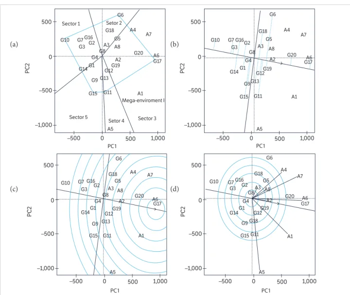
the genotypes MNC03-736F-7 (G10), MNC02-682F-2-6 (G6), BRS-Tumucumaque (G17), MNC03-737F-5-1 (G11), MNC03-737F-5-11 (G15) and MNC03-737F-5-10 (G14), which are farther away from the Biplot origin (Figure 1a). These genotypes have the largest vectors in the respective directions. The vector length and direction represent the extent of the genotypes’ response to the tested environments. All other genotypes contained in the polygon have smaller vectors, which makes them less sensitive to the interaction with the environments of each sector (Yan and Rajcan 2002). Likewise, Mattos et al. (2013) assessed the productivity of stalks of different sugarcane genotypes using the GGE Biplot methodology and found that the graphs were divided into six sectors. The polygon of the GGE Biplot (Figure 1a) grouped the A1, A2, A4, A6, A7 and A8 environments/locals into one mega-environment. Mega-environments are the sectors that contain one or more environments. The BRS-Tumucumaque (G17), which is located on the vertex of the mega-environment, had the highest average grain yield in both favorable (A6) and harsh (A2) environments. This result is reflected on its stability.

When genotypes originate the vertices of the polygon but contain no clustered environment, they are considered unfavorable to the tested environments due to low productivity (Karimizadeh et al. 2013). Thus, genotypes located in these sectors are also not recommended. In this context, except for the MNC03-736F-7 (G10), MNC02-683F-1 (G7), MNC03-737F-11 (G16), MNC02-675F-4-2 (G2), MNC02-675F-9-3 (G4), MNC02-675F-9-3 (G4) and MNC03-737F-5-10 (G14) genotypes (located in Sector 1 of Figure 1a) and MNC02-675F-4-9 (G1), MNC03-736F-7 (G10), MNC03-725F-3 (G9) and MNC03-737F-5-11 (G15) genotypes (located in Sector 5 of Figure 1a), it is possible to infer that all other genotypes have some specific adaptation and should be evaluated carefully to obtain the best recommendations.

The grain yield and stability of genotypes were evaluated by an average environment coordination (AEC) metho d. The AEC axis is repres ented by two arrows pointing in the opposite direction of the Biplot origin and indicating a greater effect of genotype × environment interaction and less stability, and even separates the genotypes that are below the average from those that are above the average. Accordingly, the BRS-Tumucumaque (G17) and MNC02-684F-5-6 y g c e E = Xb 0 0 0 ; g c e Var = lσ2 0 0 0 0 0 g lσ2 c lσ2 e 0

The model fit was obtained from the mixed model equations:

Z'X Z'W × =

X'W W'X X'X Z'y W'y X'y g c b

Z'Z + 1λ

1

W'W + 1λ 2 W'Z

X'Z ˆ

ˆ

where λ1 = σ 2 e / σ

2 g = (1 - h

2 g – c

2_)/_h2 g; λ2 = σ

2 e / σ

2 c = (1 - h

2 g – c

2_)/_h2 g,

in which h2 g = σ

2 g / (σ

2 g + σ

2 c + σ

2

e) corresponds to individual

heritability in the broad sense in the block; c2 = σ

2 c /(σ

2 g + σ

2 c + σ

2 e ),

to the determination coefficient of the genotype x environment

interaction; σ 2

g is the genetic variance among cowpea genotypes; σ 2

c is the variance of genotype x environment interaction; and, σ 2

e is the residual variance between plots. This analysis was

performed using the Selegen software (Resende 2007).

RESULTS AND DISCUSSION

(5)

(G8) genotypes were identified as being the most stable (Figure 1b), when considering the genotypes with above average productivity.

The vector length on the ideal environment axis plotted on the AEC abscissa represents an estimate of the importance of genotype main effect (G) versus the main effect of GE interaction (Yan and Rajcan 2002). The longer the vector, the more important is the genotype factor and the more significant becomes the selection based on the average performance. Then it can be seen a significant response to selection based on the average performance of the genotypes. Therefore, genotypes with productivity below average, such as MNC03-736F-7 (G10), MNC02-683F-1 (G7), MNC02-675F-9-2 (G3), MNC03-737F-5-10 (G14), among others, may be discarded.

It is also obser ved that MNC03-736F-7 (G10), 683F-1 (G7), MNC03-737F-11 (G16), MNC02-675F-4-2 (G2), MNC02-675F-9-3 (G4) and MNC03-737F-5-10 (G14) genotypes are regarded as unfavorable to the recommendation (Figure 1a). Most of these genotypes have productivity below average and are still associated with instability, justifying their undesirability. When considering the two parameters simultaneously, the recommended genotypes were BRS-Tumucumaque (G17) and BRS Guariba (G20), in descending order, because both displayed high production value, good adaptability and stability.

An ideal genotype must have an average grain yield consistently high for all environments in question. This ideal

Figure 1. Polygon (a), stability (b), ideal genotype (c) and ideal environment (d) given by the GGE Biplot method from the two main components (PC1 and PC2) for the average grain yield of the 20 erect cowpea genotypes evaluated for the eight environments described in Table 1, in Mato Grosso do Sul.

G5 A4 A4 A2 A1 A8 A3 A7 A6 G17 G20 G19 G12 G13 G15 Sector 5 Sector 1 500 0 –500 PC2 –1,000 500 0 –500 PC2 –1,000 500 0 –500 PC2 –1,000 1,000 500 –500 0 Setor 2

(6)

Identification Genotype A1 A2 A3 A4 A5 A6 A7 A8 Average

G1 MNC02-675F-4-9 1,139.5 460.5 217.0 535.3 1,585.0 1,068.5 453.8 960.0 802.4

G2 MNC02-675F-4-2 1,015.8 181.3 277.5 753.5 1,330.8 1,173.5 471.0 1,079.8 785.4

G3 MNC02-675F-9-2 993.8 210.3 153.8 372.5 1,295.0 948.5 639.3 973.8 698.3

G4 MNC02-675F-9-3 1,223.8 151.3 88.0 769.3 1,541.3 943.5 683.0 856.8 782.1

G5 MNC02-676F-3 1,250.0 404.5 135.0 719.5 1,313.8 1,078.0 1,099.3 1,093.3 886.7

G6 MNC02-682F-2-6 1,111.0 245.3 535.5 805.3 1,095.8 1,167.0 1,157.3 1,212.0 916.1

G7 MNC02-683F-1 1,208.3 335.5 396.0 361.0 1,189.0 528.3 795.5 1,139.3 744.1

G8 MNC02-684F-5-6 1,149.0 507.8 501.3 590.8 1,450.0 1,186.0 556.8 1,225.8 895.9

G9 MNC03-725F-3 1,243.8 500.5 415.5 357.5 1,817.8 1,011.0 556.5 1,092.8 874.4

G10 MNC03-736F-7 738.3 391.5 353.3 387.3 1,328.3 553.0 554.8 1,039.3 668.2

G11 MNC03-737F-5-1 1,484.0 340.0 114.0 416.0 1,909.8 1,098.5 561.5 1,356.8 910.1

G12 MNC03-737F-5-4 1,401.5 223.3 101.0 478.0 1,564.8 1,247.5 640.3 1,216.3 859.1

G13 MNC03-737F-5-9 1,519.8 226.5 148.5 589.3 1,758.5 824.8 757.8 1,162.0 873.4

G14 MNC03-737F-5-10 1,244.3 298.3 83.5 589.3 1,392.3 1,107.0 516.5 932.8 770.5

G15 MNC03-737F-5-11 1,317.3 183.3 636.8 446.0 2,090.0 834.5 596.0 1,079.0 897.8

G16 MNC03-737F-11 1,051.5 185.0 587.8 846.0 1,357.8 916.5 383.0 1,192.5 815.0

G17 BRS-Tumucumaque 1,590.8 821.3 476.3 799.3 1,624.0 1,676.5 1,138.5 1,261.0 1,173.4

G18 BRS-Cauame 1,196.5 317.0 432.8 652.0 1,127.3 1,276.5 633.0 1,534.0 896.1

G19 BRS-Itaim 1,651.0 182.0 527.8 601.8 1,451.5 1,262.5 681.0 713.0 883.8

G20 BRS-Guariba 1,481.8 294.3 274.5 807.3 1,604.3 1,269.0 1,296.0 1,225.3 1,031.5

Mean 1,250.6 323.0 322.8 593.8 1,491.3 1,058.5 708.5 1,117.3 858.2

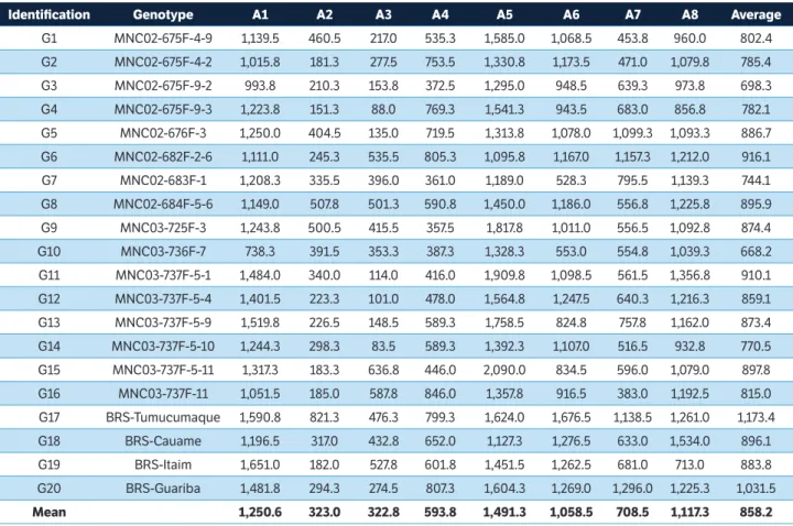
A1 = Aquidauana (2010); A2 = Chapadão do Sul (2010); A3 = Dourados (2010); A4 = Aquidauana (2011); A5 = Chapadão do Sul (2011); A6 = Dourados (2011); A7 = Aquidauana (2012); A8 = Dourados (2012).

Table 2. Average grain yield (kg∙ha–1_{) of 20 erect cowpea genotypes for each environment described in Table 1 and overall average of} environments and genotypes.

genotype is defined graphically by the longest vector in PC1 and PC2 without projections, represented by the arrow in the center of the concentric circles (Yan and Rajcan 2002) (Figure 1c). Although this genotype is more a representative model, it is used as a reference for the genotype evaluation. Thus, the BRS-Tumucumaque (G17) and BRS Guariba (G20) cultivars, placed in the first and third concentric circle, respectively, are the closest to the ideal regarding high yield and phenotypic stability.

Figure 1d shows the relationship between grain yield and stability from the vector viewpoint of environments, where the environments are connected by vectors with the Biplot origin. Environments with small vectors have high production stability. Thus, the difference between the average productivity of genotypes was lower in A3 environments (Dourados 2010), A2 (Chapadão do Sul 2010) and A8 (Dourados 2012) (Figure 1b and Table 2), i.e. they contributed less to the GE interaction. On the other hand, the A5 environment (Chapadão do Sul 2011) was the largest contributor to GE interaction.

The cosine of the angle between the two environment vectors corresponds to the coefficient of correlation between them (Yan and Rajcan 2002). Most environments were correlated positively since Figure 1d shows that the angles formed by their vectors are less than 90° (positive cosine values). The only angle > 90° is that formed by the A3 and A5 (Dourados 2010 × Chapadão do Sul 2011) vectors, with negative cosine. Likewise, Kaya and Akçura (2006) and Mattos et al. (2013) also detected positive and negative correlations between studied environments using the GGE Biplot approach to assess the interaction between wheat and sugarcane genotypes and their production environments, respectively.

(7)

Identification Genotype A1 A2 A3 A4 A5 A6 A7 A8 Average environment

MHPRVG

G1 MNC02-675F-4-9 1,307.2 517.9 414.5 668.1 1,695.3 1,174.1 720.5 1,162.6 815.8 796.2

G2 MNC02-675F-4-2 1,283.3 370.5 425.7 741.3 1,560.2 1,222.8 731.4 1,184.0 798.1 757.7

G3 MNC02-675F-9-2 1,270.8 377.6 352.1 593.8 1,533.7 1,124.4 804.3 1,152.3 724.6 670.3

G4 MNC02-675F-9-3 1,349.7 362.2 344.0 752.5 1,657.6 1,149.0 881.7 1,131.3 797.9 706.8

G5 MNC02-676F-3 1,409.7 484.9 390.2 733.0 1,574.0 1,196.0 1,048.6 1,208.7 886.7 854.0

G6 MNC02-682F-2-6 1,316.7 411.2 506.0 766.7 1,491.3 1,237.5 1,072.9 1,264.5 909.8 914.0

G7 MNC02-683F-1 1,338.0 456.4 464.5 603.4 1,518.7 1,058.5 947.2 1,219.0 764.7 755.5

G8 MNC02-684F-5-6 1,327.4 571.2 487.9 697.2 1,638.8 1,253.5 777.9 1,279.1 892.1 911.0

G9 MNC03-725F-3 1,392.0 543.2 493.3 625.6 1,801.1 1,163.1 766.8 1,200.1 884.2 871.3

G10 MNC03-736F-7 1,250.6 469.1 438.6 613.9 1,546.6 1,078.5 754.2 1,173.4 695.5 692.6

G11 MNC03-737F-5-1 1,473.3 623.7 402.0 637.2 1,844.3 1,209.3 790.6 1,348.6 934.6 863.5

G12 MNC03-737F-5-4 1,453.3 420.2 369.8 657.3 1,676.2 1,274.1 857.6 1,253.2 873.5 800.2

G13 MNC03-737F-5-9 1,485.8 436.7 379.4 687.9 1,769.5 1,100.7 988.0 1,231.3 883.3 815.5

G14 MNC03-737F-5-10 1,375.9 446.1 360.6 678.5 1,605.6 1,185.1 743.0 1,142.6 798.7 752.8

G15 MNC03-737F-5-11 1,431.8 393.9 547.7 647.0 1,900.3 1,112.1 820.3 1,192.3 896.5 844.9

G16 MNC03-737F-11 1,295.4 385.5 522.8 773.7 1,589.1 1,135.9 708.5 1,241.3 824.0 798.2

G17 BRS-Tumucumaque 1,541.7 733.1 513.7 794.6 1,744.2 1,536.1 1,099.4 1,324.6 1,135.1 1,176.5

G18 BRS-Cauame 1,361.7 428.5 478.1 721.3 1,504.8 1,327.6 838.3 1,403.1 892.3 888.9

G19 BRS-Itaim 1,533.0 402.4 499.3 708.2 1,623.4 1,295.8 911.2 1,117.2 887.0 859.8

G20 BRS-Guariba 1,502.6 499.8 451.4 783.8 1,720.7 1,386.0 1,138.8 1,299.9 1,020.1 1,007.8

Environment overall average 1,385.0 466.7 442.1 694.3 1,649.8 1,211.0 870.1 1,226.5 865.7 ---Table 3. Genotypic values, as well as adaptability and stability of genotypic values (MHPRVG) predicted by the analysis REML/BLUP for grain

yield (kg∙ha–1_{) of 20 erect cowpea genotypes for each tested environment, and overall average of environments.}

A1 = Aquidauana (2010); A2 = Chapadão do Sul (2010); A3 = Dourados (2010); A4 = Aquidauana (2011); A5 = Chapadão do Sul (2011); A6 = Dourados (2011); A7 = Aquidauana (2012); A8 = Dourados (2012).

serves as a reference for selecting sites for multi-environment trials. Thus, according to the GGE Biplot method, the A2 (Chapadão do Sul 2010) and A6 (Dourados 2011) environments were those that displayed higher ability to discriminate genotypes. Thus, in environments with similar soil and climatic conditions, the municipalities of Chapadão do Sul and Dourados are indicated for the selection of cowpea genotypes.

However, it should be taken into account that the GGE Biplot method captures only a small percentage of the total variability, which may compromise the analysis since the obtained standards display less precision, requiring, therefore, the use of mixed models (Yang et al. 2009). The mixed-model approach, REML/BLUP, provides results that are interpreted directly as a genotypic values, already capitalized or penalized by the stability and adaptability estimates (Silva et al. 2011).

The BRS-Tumucumaque and BRS-Guariba cultivars had the best genotypic values across the environments and the average environment according to the REML/BLUP analysis (Table 3). These cultivars are also the best according to the harmonic mean of the MHPRVG, which simultaneously selects genotypes with high grain yield, adaptability, and stability, although it does not inform the most similar places. Thus, it is highlighted that the two methods tested, GGE Biplot and REML/BLUP, were in agreement regarding the results for indicating the best genotypes, which has been observed by Silva et al. (2011) as well.

(8)

Cruz, C. D., Carneiro, P. C. S. and Regazzi, A. J. (2014). Modelos biométricos

aplicados ao melhoramento genético. 3. ed. Viçosa: Editora da UFV.

Karimizadeh, R., Mohammadi, M., Sabaghni, N., Mahmoodi, A. A.,

Roustami, B., Seyyedi, F. and Akbari, F. (2013). GGE Biplot analysis

of yield stability in multienvironment trials of lentil genotypes under

rainfed condition. Notulae Scientia Biologicae, 6, 256-262.

Kaya, Y. M. and Akçura, T. S. (2006). GGE-Biplot analysis of

multi-environment yield trials in bread wheat. Turkish Journal of Agriculture

and Forestry, 30, 325-337.

Mattos, P. H. C., Oliveira, R. A., Bespalhok Filho, C., Daros, E. and

Veríssimo, M. A. A. (2013). Evaluation of sugarcane genotypes

and production environments in Paraná by GGE Biplot and AMMI

analysis. Crop Breeding and Applied Biotechnology, 13, 83-90.

http://dx.doi.org/10.1590/S1984-70332013000100010.

Miranda, G. V., Souza, L. V., Guimarães, L. J. M., Namorato, H.,

Oliveira, L. R. and Soares, M. O. (2009). Multivariate analyses

of genotype × environment interaction of popcorn. Pesquisa

Agropecuária Brasileira, 44, 45-50. http://dx.doi.org/10.1590/

S0100-204X2009000100007.

Nascimento, S. P., Bastos, E. A., Araújo, E. C. E., Freire Filho, F. R. and

Silva, E. M. (2011). Tolerância ao déficit hídrico em genótipos de

feijão-caupi. Revista Brasileira de Engenharia Agrícola e Ambiental,

15, 853-860. http://dx.doi.org/10.1590/S1415-43662011000800013.

R Development Core Team (2014). R: a language and environment

for statistical computing; [accessed 2016 May 23].

http://www.R-project.org

Resende, M. D. V. (2007). SelegenREML/BLUP: sistema estatístico

e seleção genética computadorizada via modelos lineares mistos.

Colombo: Embrapa Florestas.

REFERENCES

Rosado, A. M., Rosado, T. B., Alves, A. A., Laviola, B. G. and Bhering,

L. L. (2012). Seleção simultânea de clones de eucalipto de acordo

com produtividade, estabilidade e adaptabilidade. Pesquisa

Agropecuária Brasileira, 47, 964-971. http://dx.doi.org/10.1590/

S0100-204X2012000700013.

Santos, J. A. S., Soares, C. M. G., Corrêa, A. M., Teodoro, P. E.,

Ribeiro, L. P. and Abreu, H. K. A. (2014). Agronomic performance

and genetic dissimilarity among cowpea (Vigna unguiculata (L.)

Walp.) genotypes. Global Advanced Research Journal of Agricultural

Science, 3, 271-277.

Silva, G. O., Carvalho, A. D. F., Veira, J. V. and Benin, G. (2011).

Verificação da adaptabilidade e estabilidade de populações

de cenoura pelos métodos AMMI, GGE Biplot e REML/

BLUP. Bragantia, 70, 494-501. http://dx.doi.org/10.1590/

S0006-87052011005000003.

Yan, W., Hunt, L. A., Sheng, Q. L. and Szlavnics, Z. (2000). Cultivar

evaluation and mega-environment investigation based on the

GGE Biplot. Crop Science, 40, 597-605. http://dx.doi.org/10.2135/

cropsci2000.403597x.

Yan, W. and Rajcan, I. (2002). Biplot evaluation of test sites and

trait relations of soybean in Ontario. Crop Science, 42, 11-20. http://

dx.doi.org/10.2135/cropsci2002.0011.

Yang, R. C., Crossa, J., Cornelius, P. L. and Burgueño, J. (2009).

Biplot analysis of genotype × environment interaction: proceed

with caution. Crop Science, 49, 1564-1576. http://dx.doi.org/10.2135/

cropsci2008.11.0665.

Yates, F. and Cochran, W. G. (1938). The analysis of groups of

experiments. The Journal of Agriculture Science, 28, 556-580.

http://dx.doi.org/10.1017/S0021859600050978.

CONCLUSION

There was agreement of the two methods investigated, GGE Biplot and REML/BLUP, regarding the identification of the best cowpea genotypes indicated for the conditions in Mato Grosso do Sul.