ABSTRACT:Sugarcane (Saccharum sp.) is one of the most important crops in Brazil. The high demand for sugarcane-derived products has stimulated the expansion of sugarcane cultivation in recent years, exploring different environments. The adaptability and the phenotypic stability of sugarcane genotypes in the Minas Gerais state, Brazil, were evaluated based on the addi-tive main effects and multiplicaaddi-tive interaction (AMMI) method. We evaluated 15 genotypes (13 clones and two checks: RB867515 and RB72454) in nine environments. The average of two cut-tings for the variable tons of pol per hectare (TPH) measure was used to discriminate genotypes. Besides the check RB867515 (20.44 t ha–1), the genotype RB987935 showed a high average TPH (20.71 t ha–1), general adaptability and phenotypic stability, and should be suitable for cul-tivation in the target region. The AMMI method allowed for easy visual identification of superior genotypes for each set of environments.
Keywords: G × E interaction, principal components, multivariate analysis
Introduction
Sugarcane (Saccharum sp.) is one of the most im-portant crops in Brazil, and is the source of a large number of products, including sugar and ethanol. In addition, the bagasse residue from the industry has also gained importance in the co-generation of elec-tricity. The high demand for these products has pro-vided significant impetus to the expansion of sugar-cane cultivation in recent years.
In the last crop season (2010/11), the area under cultivation increased 8.4 % in Brazil. Increases were re-corded in all producing regions of the country (CONAB, 2011). The outlook for coming years is brighter than in previous years. Minas Gerais state, which has the sec-ond largest cultivated area and the highest yields, has expanded its area of cultivation at levels above the na-tional mean (CONAB, 2011). Because of the expansion of the crop in varied agro-climatic conditions it is very common to get different relative performances from the same cultivars when they are evaluated in different en-vironments or in different years. The variations that oc-cur in the performance of cultivars are attributed to the effect of the genotype × environment (G × E) interac-tion (Haldane, 1946; Falconer and Mackay, 1996). The selection of genotypes to maximise yield when genotype rank changes occur across environments is complicated because of the complexity of genotype responses. This type of interaction reduces selection efficiency and the accuracy of cultivar recommendation (Crossa and Cor-nelius, 1997).
Several statistical methods are available to mini-mise the effect of the G × E interaction on the selec-tion of cultivars and the predicselec-tion of the phenotypic response to environmental changes. Among the most
common methods are linear regression analysis, non-lin-ear regression analysis, multivariate analysis and non-par-ametric statistics (Cornelius et al., 1996; Annicchiarico, 1997; Moreno-González et al., 2004). In recent years, the quantification of G × E interactions and yield stability studies involving sugarcane have been done through multivariate procedures, such as principal component analysis (Kumar et al., 2009; Guerra et al., 2009; Rea et al., 2011).
The additive main effect and multiplicative inter-action (AMMI) method integrates analysis of variance (ANOVA) and principal component analysis (PCA) into a unified approach that can be used to analyse multi-location trials (Zobel et al., 1988; Crossa et al., 1990; Gauch and Zobel, 1996). AMMI uses analysis of vari-ance to study the main effects of genotypes and envi-ronments and a principal component analysis for the residual multiplicative interaction among genotypes and environments. AMMI provides the G × E interaction sum of squares (SSG×E) with a minimum number of de-grees of freedom.
In addition, AMMI simultaneously quantifies the contribution of each genotype and environment to the SSG×E, and provides an easy graphical interpretation of the results by the biplot technique to simultaneously classify genotypes and environments (Kempton, 1984; Zobel et al., 1988). Therefore, with this technique, one can readily identify productive cultivars with wide adaptability or mega-environments, as well as delimit the agronomic zoning of cultivars with specific adapt-ability and identify environments in which to conduct tests (Kempton, 1984; Gauch and Zobel, 1996; Ferreira et al., 2006). This study aimed to evaluate the adaptabil-ity and phenotypic stabiladaptabil-ity of sugarcane genotypes in Minas Gerais state, Brazil, using the AMMI method. Received November 19, 2011
Accepted March 25, 2012
1UFPR – Depto. de Fitotecnia e Fitossanitarismo, R. dos Funcionários, 1540, C.P. 19061 – 81531-990 – Curitiba, PR – Brasil.
2UFV – Depto. de Fitotecnia, Av. P.H. Rolphs, s/n – 36570-000 – Viçosa, MG – Brasil. 3UFV – Depto. de Estatística.
*Corresponding author <[email protected]>
Edited by: Antonio Costa de Oliveira
AMMI analysis to evaluate the adaptability and phenotypic stability of sugarcane
Luís Cláudio Inácio da Silveira1, Volmir Kist2, Thiago Otávio Mendes de Paula2, Márcio Henrique Pereira Barbosa2*, Luiz Alexandre
Peternelli3, Edelclaiton Daros1
Materials and Methods
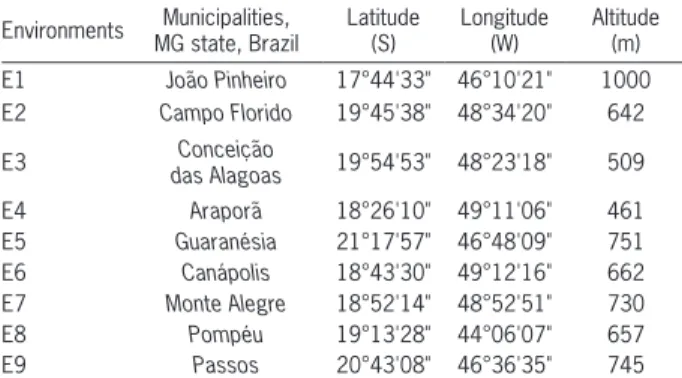
In 2005 and 2006, we evaluated 15 genotypes of sugarcane (13 clones and two checks: RB867515 and RB72454) in nine environments in Minas Gerais state, Brazil. The checks had been recommended for produc-tion on soils of medium fertility. Therefore, they have been widely cultivated in all producing regions of Brazil. RB867515, which was developed by the Sugarcane Breed-ing Program of the Federal University of Viçosa (UFV), particularly, has been cultivated around 1.6 million ha, corresponding to approximately 20 % of the commercial sugarcane crop in the country. Regarding the environ-ments, a brief description can be found on Table 1.
The experiments were conducted in a randomised complete-block design with three replications and were carried out between Feb. and Mar. 2004. The experimen-tal unit consisted of four 10 m long rows, with a spacing of 1.4 m between rows and with a distribution of 18 buds m–1.
The sugarcane stalks were harvested in Aug. 2005 (first cut) and in the same month in 2006 (second cut). The stalks were harvested after burning the straw. Weighing was done in the field using a dynamometer. From the val-ues of the weight of stalks (kg) per plot, tons of stalks per hectare (TSH) were estimated. The pol content (PC) was obtained from juice analysis of ten stalks from each plot. Therefore, the variable tons of pol per hectare (TPH) was obtained as follows: TPH = (TSH × PC)/100
To discriminate among the genotypes, mean val-ues of TPH were obtained from the first and second cut. Initially, an individual analysis of variance by environ-ment was performed. Subsequently, a combined analy-sis of variance was conducted, considering the effect of genotype as fixed and environment as random, accord-ing to the followaccord-ing statistical model:
Yijk = m + B/Ejk + Gi + Ej + GEij + εijk,
where Yijk represents the ith genotype in the jth
en-vironment and the kth block; m is the overall mean;
B/Ejk corresponds to the block within the jth
environ-ment and in the kth block; G
i is the effect of the i th
genotype; Ej is the effect of the jth environment; GE ij
is the effect of interaction of the ith genotype with the
jth environment; and ε
ijk is the effect of experimental
error. The homogeneity of residual variances was veri-fied by the ratio between the larger and smaller mean square error (MSE) as described in Cruz et al. (2004). Finally, adaptability and phenotypic stability analyses were performed by the AMMI method as described in Zobel et al. (1988) using the following statistical model:
Yij = µ + gi + ej + n
n K=
∑
λkαikyjk + rij + εij,where Yij is the mean response of genotype i in the environment j; µ is the overall mean; gi is the fixed effect of genotype i (i = 1, 2, ... g); ej is the random effect of environment j (j = 1, 2, ... e); εij is the av-erage experimental error; the G × E interaction is represented by the factors; λk is a unique value of the kth interaction principal component analysis (IPCA),
(k = 1, 2, ... p, where p is the maximum number of estimable main components), αik is a singular value for the ith genotype in the kth IPCA, y
jk is a unique
value of the jth environment in the kth IPCA; r ij is
the error for the G × E interaction or AMMI residue (noise present in the data); and k is the characteristic non-zero roots, k = [1, 2, ... min (G - 1, E - 1)].
The sum of squares for the G × E interaction (SSG×E) was divided into n singular axes or main com-ponents of interaction (IPCA), which was described the standard portion, each axis corresponding to an AMMI model. The choice of model that best described the G × E interaction was done based on the FR test proposed by Cornelius et al. (1992).
After selecting the AMMI model, a study of adapt-ability and phenotypic stadapt-ability of the biplot graphic was designed. This graphic was obtained by the com-binations of the orthogonal axis of the IPCAs. The bi-plot term refers to a type of graphic that contains two categories of points or markers. In this study, it refers to genotypes and environments. The biplot graphic in-terpretation was based on the variation caused by the main additive effects of genotype and environment, and the multiplicative effect of the G × E interaction. The abscissa represents the main effects (overall aver-age of the variables of the genotypes evaluated) and the ordinate is the first interaction axis (IPCA1). In this case, the lower the IPCA1 value (absolute values), the lower its contribution to the G × E interaction; there-fore, the more stable the genotype. The ideal genotype is one with high productivity and IPCA1 values close to zero. An undesirable genotype has low stability associ-ated with low productivity (Kempton, 1984; Gauch and Zobel, 1996; Ferreira et al., 2006). Finally, the predic-tive averages were estimated according to the selected model. All statistical analyses were conducted using SAS 9.0 (SAS Institute, 2002).
Table 1 – Locations where the experiments were conducted with 15 genotypes of sugarcane, in the crop seasons 2004/05 and 2005/06.
Environments Municipalities, MG state, Brazil
Latitude (S)
Longitude (W)
Altitude (m) E1 João Pinheiro 17°44'33" 46°10'21" 1000 E2 Campo Florido 19°45'38" 48°34'20" 642
E3 Conceição
Results and Discussion
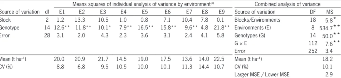
The individual analyses of variance revealed dif-ferences (p ≤ 0.05) among genotypes in all environ-ments, except in E8. Nevertheless, there was sufficient genetic variability to be exploited by selection (Table 2). The combined analysis of variance showed highly differences (p≤ 0.01) for environments (E), genotypes (G) and the G × E interaction (Table 2). The experi-mental coefficients of variation (CV) were relatively low (6.8 % to 14.4 % in the individual ANOVA and 10.1 % in the combined ANOVA), indicating good ex-perimental precision. The ratio between the larger and the lower mean square error (MSE) from the individual ANOVA was 2.9 (Table 2), indicating that the combined ANOVA could be performed.
The significant effect of the G × E interaction revealed that the genotypes had variable performance in the tested environments, i.e., a change in the av-erage rank of the genotypes was verified among the environments, justifying the conduction of a more refined analysis so that to increase the efficiency of the selection and indication of cultivars. In this sense, AMMI analysis represents a potential tool that can be used to deepen the understanding of factors involved in the manifestation of the G × E interaction. Through this, it was estimated that the effect of the G × E interaction through multivariate analysis (principal components analysis, PCA and singular-value decom-position, SVD) could describe the pattern adjacent to the data from an interaction matrix (G × E), making the decomposition of the sum of squares of the G × E interaction (SSG×E) in axis or interaction principal components analysis (IPCA).
The AMMI model recovers the part of SSG×E that determines the G × E interaction, which is called the standard part (effect of genotypes and environments) and a residual part, which corresponds to unpredictable and uninterpretable responses (Crossa et al., 1990). In this case, the genetic variance can be explained by the dif-ferent models of AMMI, which can be: AMMI0, which does not include any axis or interaction term; AMMI1,
which includes only the first interaction axis; AMMI2 which involves the first two axis, and so on (Cornelius et al., 1996).
The greatest percentage of the pattern is retained in the first singular axis; in the subsequent axis, this value will gradually decrease. On the other hand, this increases noise retention (Gauch and Zobel, 1988). Thus, for greater accuracy in the information, it is desirable that most of the structural pattern of SSG×E be captured in the first axis.
The AMMI analysis of variance of TPH across two cuttings and nine environments showed that 73.36 % of the total SS was attributable to environmental effects, 12.01 % to genotypic effects and 14.63 % to G × E in-teraction effects (Table 3). A large SS for environments indicated that the environments were diverse, with large differences among environmental means causing most of the variation in TPH.
Based on the FR test of Cornelius et al. (1992), only IPCA1 was significant (p≤ 0.01) (Table 3). There-fore, the AMMI2 model was selected to explain the ef-fect of the G × E interaction. According to Cornelius
Table 2 – Means squares of individual analysis of variance, summary of the combined analysis of variance, means, coefficients of variation (CV) and the coefficient of the relationship between the larger and lower MSE for the variable TPH of 15 genotypes in nine environments in Minas Gerais State, Brazil, in the crop seasons of 2005 and 2006.
Means squares of individual analysis of variance by environment(a) Combined analysis of variance
Source of variation df E1 E2 E3 E4 E5 E6 E7 E8 E9 Source of variation DF MS
Block 2 1.2 13.3 10.5 1.0 0.8 7.1 10.4 7.8 0.1 Blocks/Environments 18 5.8*
Genotype 14 12.6** 11.8** 10.1* 7.9** 16.5** 15.8** 9.6** 4.8 21.8** Environments (E) 8 534.7**
Error 28 3.1 2.0 4.3 2.3 3.6 3.1 2.4 4.1 5.8 Genotypes (G) 14 50.0**
G × E 112 7.6**
Error 252 3.4
Mean (t ha–1) 20.0 20.9 21.7 14.5 19.0 17.5 13.6 14.0 22.5 Mean (t ha–1) 18.2
CV (%) 8.8 6.8 9.5 10.5 10.0 10.1 11.3 14.4 10.7 CV (%) 10.1
Larger MSE / Lower MSE 2.9
(a) E1: João Pinheiro; E2: Campo Florido; E3: Conceição das Alagoas; E4: Araporã; E5: Guaranésia; E6: Canápolis; E7: Monte Alegre; E8: Pompéu; E9: Passos. NS, *, **non-significant, significant at p > 0.05 and p > 0.001 by F test, respectively.
Table 3 – Summary of analysis of variance and partitioning of the G × E interaction by the AMMI method, the explained variance and its accumulated value for the TPH variable.
Source DF SS MS Explained Accumulated
% ---Environments (E) 8 4277.58 534.70**
Genotypes (G) 14 700.24 50.02**
G × E 112 853.18 7.62**
IPCA1 91 559.98 6.15** 34.36 34.36
IPCA2 72 368.76 5.12NS 22.42 56.78
IPCA3 55 215.19 3.91NS 18.00 74.78
IPCA4 40 124.57 3.11NS 10.62 85.40
IPCA5 27 69.38 2.57NS 6.47 91.87
IPCA6 16 32.06 2.00NS 4.37 96.24
IPCA7 7 8.39 1.20NS 2.78 99.02
IPCA8 0 0 0 0.98 100.00
Error 252 859.51 3.41
et al. (1992), a multiplicative term (n + 1) should be added to the previously adjusted terms (n terms). Thus, it was possible to explain 56.78 % of the interaction sum of squares, at 34.36 % and 22.42 % for IPCA1 and IPCA2, respectively. The value explained by these first two IPCAs presents the same magnitude as those found by Guerra et al. (2009), using the same variable evalu-ated in sugarcane genotypes in the Paraná state, Bra-zil. Note that the explanation of the interaction sum of squares could be enhanced if one adds more IPCAs to the model. However, as commented by Piepho (1995), this option may be dangerous because it may also in-crease the influence of noise.
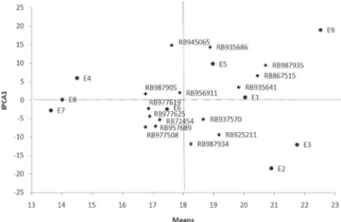
To illustrate the effect of each genotype and environment, the AMMI1 (IPCA1 vs. means) (Figure 1) and AMMI2 (IPCA2 vs. IPCA1) (Figure 2) biplots are shown. In Figure 1, the x-coordinate indicates the main effects (means) and the y-coordinate indicates the effects of the interaction (IPCA1). Values closer to the origin of the axis (IPCA1) provide a smaller
con-tribution to the interaction than those that are further away. In this case (Figure 1), it appears that genotypes RB956911, RB977619 and RB967905 showed greater stability. However, their averages were among the lowest, and, therefore, these genotypes should not be recommended. On the other hand, the genotypes RB945065 and RB935686 were the most unstable, with averages close to the overall average. In turn, the majority of genotypes occupied an intermediate position, relatively similar to the checks (RB72454 and RB867515). However, among these genotypes, RB987935 could be highlighted. This genotype had the highest average TPH and stability comparable to the check RB867515, which is the cultivar most widely grown throughout Brazil. The genotypes RB935641, RB925211 and RB937570 also had good average TPH values (> 18 t ha–1).
Some of the environments stood out with a small contribution to the interaction (E1 and E8); with an intermediate contribution (E4, E5, E6 and E7); and with a high contribution (E2, E3 and E9) (Figure 1). Only in environments E1, E2, E3, E5 and E9, averages were recorded above the overall averages (18 t ha–1),
indicating that these were favourable environments to obtain high means. The main reason for these high TPH means in these cited environments is the good precipitation and water distribution that occurs dur-ing the crop cycle, besides the relatively higher nat-ural fertility of these soils compared with the other environments.
The genotypes RB956911, RB977619 and RB967905 were the most stable; however, these were in company with the genotypes RB937570, RB977508 and RB957689 and the check RB72454 (Figure 2). This conclusion holds because these genotypes were po-sitioned near the origin of the biplot. On the other hand, genotypes RB935686, RB935641, RB987934 and RB977625 were the most unstable; that is, these had specific adaptations, because they were more distant from the biplot origin.
Environment E8 was the largest contributor to the phenotypic stability of these genotypes (Figure 2). It was in this environment that no differences (p > 0.05) were found among genotypes via the individual ANOVA. Additionally, this environment recorded one of the lowest TPH means. On the other hand, environ-ments E2, E6, E7 and E9 mostly contributed to the G × E interaction, because they were positioned far from the origin in the AMMI2 biplot.
Genotypes and environments positioned close to each other in the biplot have positive associations, thus these enable the creation of agronomic zones with rela-tive ease. Genotype RB977625 had a specific adapta-tion to environment E7, whereas genotypes RB945056, RB987935 and the check RB867515 were adapted to en-vironment E5 and RB935686 to enen-vironment E9. Other associations between genotypes and environments can be seen in Figure 2.
Figure 1 – AMMI1 biplot showing the IPCA1 vs. means for the TPH variable of 15 genotypes evaluated in nine environments in Minas Gerais State, Brazil, in 2005 and 2006.
In general, we sought to have cultivars with wide geographic adaptation with high productivity and which can assure a good mean TPH (> 18 t ha–1), even
if the environments to be cultivated are very hetero-geneous. However, because this condition is hardly achieved, to increase regional productivity, it is impor-tant that genotypes with specific adaptations also be identified. Particularly in sugarcane, the identification of these specific positive interactions becomes espe-cially important because the renewal of the sugarcane fields usually happens after a long period of six or seven cuts (years). Thus, when a new cultivar is erroneously recommended, the economic damage may be extended for many years.
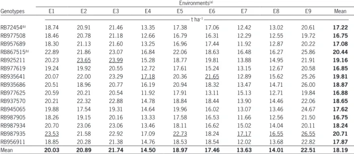
Classifying environments based on the winning genotypes (raw data), i.e., those with the highest means in each environment (Gauch and Zobel, 1997), six mega-environments were formed (RB987935 in E1, E5 and E8; RB925211 in E2; RB935641 in E4 and E6; RB937570 in E3; RB987934 in E7; RB867515 in E9). On the other hand, based on the predicted means obtained from AMMI2 (FR Cornelius), three mega-environments were formed. The first one contains environments E2 and E3, with geno-type RB925211 as the winner. The second one contains E4 and E6, genotype RB935641 being the best in these environments. The last mega-environment was formed by environments E1, E5, E7, E8 and E9, where genotype RB987935 was the winner (Table 4). The superiority of mega-environments formed from the raw means can be attributed to the noise that is embedded in these estimates. If proper care is not taken, erroneous recommendations of cultivars can be made involuntarily. In this sense, the statistical AMMI approach delivers less biased results.
Comparing cultivar recommendations based on the raw means (20.7 t ha–1) of the winning genotype
(RB987935), an increase of 13.8 % would be obtained while less would be obtained based on the experiment mean (18.2 t ha–1). If we consider specific adaptations
based on the raw means (six winning genotypes), the predicted mean TPH was 21.9 t ha–1, corresponding
to an increase of 20.7 % above the mean of the ex-periment. Considering the predicted means from the AMMI1 analysis, the formation of two mega-environ-ments could be verified by the two genotype winners (RB925211 in E2 and E3, RB987935 in the other envi-ronments). The expected average TPH from this mod-el is 21 t ha–1, i.e. an increase of 15.4 % over the mean
of the experiment. From a practical point of view, AMMI1 should be adopted instead of the raw mean of each environment because the former results in a smaller number of mega-environments. However, the AMMI2 family was more predictive than any other (FR Cornelius). Therefore, we would have three mega-environments with an expected average TPH of 21.4 t ha–1, which resulted in an increase of 17.9 %
com-pared to the raw mean.
The estimates obtained from a large number of mega-environments result in high means; however, these are often biased. On the other hand, with a minor number of mega-environments (as indicated by AMMI2) one could obtain mean estimates that are less biased than those obtained from a large number of mega-envi-ronments.
Besides providing a more secure statistical inter-pretation of the results, since it contains a part of the recovered genetic SSG×E effects, the AMMI analysis al-lowed us to make an easy and practical interpretation of the results. Therefore, it was possible to identify the most stable genotypes and also those that were highly productive and adapted to specific environments.
Table 4 – Predicted means by the AMMI2 model for the TPH variable.
Environments(a)
Genotypes E1 E2 E3 E4 E5 E6 E7 E8 E9 Mean
--- t ha–1
---RB72454(b) 18.74 20.91 21.46 13.35 17.38 17.06 12.42 13.02 20.61 17.22
RB977508 18.46 20.78 21.18 12.66 16.79 16.31 12.29 12.55 19.72 16.75
RB957689 18.30 21.13 21.60 13.25 16.96 17.44 11.92 12.87 20.22 17.08
RB867515(b) 22.89 21.86 23.07 16.84 22.06 18.63 16.48 16.27 25.86 20.44
RB925211 20.23 23.65 23.99 15.28 18.77 19.81 13.88 14.95 21.91 19.16
RB977619 19.24 19.92 20.55 12.72 17.61 15.24 13.15 12.67 20.58 16.85
RB935641 20.07 22.00 23.29 17.18 20.36 21.65 12.89 15.62 25.26 19.81
RB935686 20.51 18.96 20.77 16.19 20.94 18.32 13.47 14.71 26.00 18.87
RB977625 20.59 20.21 20.54 11.92 17.91 13.11 15.13 12.71 19.84 16.88
RB937570 20.21 22.32 22.88 14.78 18.84 18.44 13.90 14.46 22.06 18.65
RB945065 19.88 17.54 19.31 14.64 19.96 16.02 13.07 13.46 24.67 17.62
RB987905 18.26 19.15 20.16 13.33 17.58 16.53 11.66 12.56 21.50 16.75
RB987934 20.70 23.06 23.06 13.46 18.11 16.62 15.02 14.04 20.11 18.24
RB987935 23.53 21.58 22.92 17.09 22.73 18.24 17.17 16.55 26.55 20.71
RB956911 18.85 20.28 21.38 14.76 18.53 18.54 12.02 13.68 22.82 17.87
Mean 20.03 20.89 21.74 14.50 18.97 17.46 13.63 14.01 22.51 18.19
Conclusions
Genotype RB987935 may be more suitable for commercial cultivation;
Environment E8 should be used for the conduc-tion of preliminary tests in the selecconduc-tion scheme;
Genotypes RB925211, RB937570, RB935641, RB935686 and RB987935 and the check RB867515 show high productivity and specific adaptation to environ-ments E3, E6, E9 and E5, respectively;
Safely identifying G × E interactions provides a positive indication of highly responsive cultivars, which can significantly improve crop productivity in specific regions.
Acknowledgments
The authors thank the mills and distilleries of the State of Minas Gerais for financial support for the Sugarcane Breeding Program of the Federal Univer-sity of Viçosa, MG, Brazil, the InteruniverUniver-sity Net-work for Developing the Sugar and Alcohol Industry (RIDESA) for providing the clones used in this re-search, the Fundação de Amparo à Pesquisa do Es-tado de Minas Gerais (FAPEMIG) and the Conselho Nacional de Desenvolvimento Científico e Tecnológico (CNPq) for financial support of the students involved in this research.
References
Annicchiarico, P. 1997. Joint regression vs AMMI analysis of genotype-environment interactions for cereals in Italy. Euphytica 94: 53–62.
Companhia Nacional de Abastecimento [CONAB]. 2011. Agricultural information Center. Harvest: sugarcane. Available at: http://www.conab.gov.br [Accessed Feb. 25, 2011] (in Portuguese).
Cornelius, P.L.; Crossa, J.; Seyedsadr, M.S. 1996. Statistical tests and estimators of multiplicative models for genotype-by-environment interaction. p. 199–234. In: Kang, M.S.; Gauch, H.G., eds. Genotype-by-environment interaction. CRC Press, Boca Raton, FL, USA.
Cornelius, P.L.; Seyedsadr, M.; Crossa, J. 1992. Using the shifted multiplicative model to search for “separability” in crop cultivar trials. Theorical and Applied Genetics 84: 161–172.
Crossa, J.; Cornelius, P.L. 1997. Sites regression and shifted multiplicative model clustering of cultivar trial sites under heterogeneity of errors variances. Crop Science 37: 406–415.
Crossa, J.; Gauch, H.G.; Zobel, R.W. 1990. Additive main effects and multiplicative analysis of two international maize cultivar trials. Crop Science 30: 493–500.
Cruz, C.D.; Regazzi, A.J.; Carneiro, P.C.S. 2004. Biometric Models Applied to Breeding. 3ed. UFV, Viçosa, MG, Brazil (in Portuguese).
Falconer, D.S.; Mackay, T.F.C. 1996. Introduction to Quantitative Genetics. 4ed. London: Longman Scientific and Technical, Essex, England.
Ferreira, D.F.; Demétrio, C.G.B.; Manly, B.F.J.; Machado, A.A.; Vencovsky, R. 2006. Statistical models in agriculture: biometrical methods for evaluating phenotypic stability in plant breeding. Cerne 12: 373–388.
Gauch, H.G.; Zobel, R.W. 1988. Predictive and postdictive success of statistical analysis of yield trial. Theoretical and Applied Genetics 76: 1–10.
Gauch, H.G.; Zobel, R.W. 1996. AMMI analysis of yield trials. Chap. 4. p. 85–122. In: Kang, M.S.; Gauch, H.G., eds. Genotype by environment interaction. CRC Press, Boca Raton, FL, USA. Gauch, H.G.; Zobel, R.W. 1997. Identifying mega-environments
and targeting genotypes. Crop Science 37: 311–326.
Guerra, E.P.; Oliveira, R.A.; Daros, E.; Zambon, J.L.C.; Ido, O.T.; Bespalhok Filho, J.C. 2009. Stability and adaptability of early maturing sugarcane clones by AMMI analysis. Crop Breeding and Applied Biotechnology 9: 260–267.
Haldane, J.B.S. 1946. The interaction of nature and nurture. Annals of Eugenics 13: 197–205.
Kempton, R.A. 1984. The use of biplots in interpreting variety by environment interactions. Journal of Agricultural Science 103: 123–135.
Kumar, S.; Hasan, S.S.; Singh, P.K.; Pandey, D.K.; Singh, J. 2009. Interpreting the effects of genotype × environment interaction on cane and sugar yields in sugarcane based on the AMMI model. Indian Journal of Genetics 3: 225–231.
Moreno-González, J.; Crossa, J.; Cornelius, P.L. 2004. Genotype × environment interacion in multi-environment trials using shrinkage factors for AMMI models. Euphytica 137: 119–127.
Piepho, H.P. 1995. Robustness of statistical test for multiplicative terms in the additive main effects and multiplicative interaction model for cultivar trial. Theoretical and Applied Genetics 90: 438–443.
Rea, R.; Sousa-Vieira, O.; Ramón, M.; Alejos, G.; Díaz, A.; Briceño, R. 2011. AMMI analysis and its application to sugarcane regional trials in Venezuela. Sugar Tech 1–6. DOI: http://dx.doi.org/10.1007/s12355-011-0070-8
SAS Institute. 2002. SAS/STAT Software: changes and enhancements through release 6.12. SAS Institute, Cary, NC, USA.