Glauco Gomes de Azevedo
Distance Estimation for Mixed Continuous and
Categorical Data with Missing Values
Rio de Janeiro
2018
Glauco Gomes de Azevedo
Distance Estimation for Mixed Continuous and
Categorical Data with Missing Values
Dissertação submetida à Escola de
Matemática Aplicada como requisito
parcial para a obtenção do grau de Mestre em Modelagem Matemática.
Fundação Getulio Vargas – FGV Escola de Matemática Aplicada – EMAp Programa de Mestrado em Modelagem Matemática
Supervisor: Eduardo Fonseca Mendes
Rio de Janeiro
2018
Azevedo, Glauco Gomes de
Distance Estimation for Mixed Continuous and Categorical Data with Missing Values/ Glauco Gomes de Azevedo. – 2018.
51f.
Dissertação (Mestrado) – Fundação Getulio Vargas, Escola de Matemática Apli-cada.
Orientador: Eduardo Fonseca Mendes Inclui bibliografia.
1. Aprendizado do computador. 2. Ausência de dados (Estatística). 3. Modelagem de dados. I. Mendes, Eduardo Fonseca. II. Fundação Getulio Vargas. Escola de Matemática Aplicada. III. Distance Estimation for Mixed Continuous and Categorical Data with Missing Values.
Acknowledgements
Português
Meus agradecimentos são para todos que acreditaram no meu potencial e na minha vontade de descobrir mais sobre ciências, principalmente a minha mãe Sonia G. Santos, meu pai Adilson O. Azevedo e a minha avó Lucy, que sempre me deram o conforto com o que pude levar adiante meus estudos por mais tempo. Devo prestar minha gratidão também aos meu caros orientadores, Prof. Dr. Milton Ramos Ramirez, de minha graduação na IM/UFRJ, e ao Prof. Dr. Eduardo Fonseca Mendes, meu orientador durante este projeto na FGV/EMAp, por sua paciência e disposição em me ensinar tanto sobre tudo que precisei saber ao longo dessa formação acadêmica. Por fim, em especial, meus agradecimentos à Priscila R. S. A. Rêgo, por ter acompanhado boa parte de minha jornada na busca pelo meu título de mestre e me ajudado com muitos bons conselhos.
English
My thanks goes to all people who believed in my potential and my will to discover more about science. Firstly to my mother Sonia G. Santos, my father Adilson O. Azevedo and to my grandmother Lucy, who always gave me the support which let me go further in my academic time. Also, I must thank my undergratuation supervisor at IM/UFRJ, Prof. Dr. Milton Ramos Ramirez, and my graduation supervisor through this work at FGV/EMAp, Prof. Dr. Eduardo Fonseca Mendes, for their patience and goodwill in teaching me all I needed to know along my courses. At last, I give my special thanks to Priscila R. S. A. Rêgo, for following my journey in the seek of my master degree, helping me with wisdon and great advices.
Resumo
Neste trabalho é proposta uma metodologia para estimar distâncias entre pontos de dados mistos, contínuos e categóricos, contendo dados faltantes. Estimação de distâncias é a base para muitos métodos de regressão/classificação, tais como vizinhos mais próximos e análise de discriminantes, e para técnicas de clusterização como k-means e k-medoids. Métodos clássicos para manipulação de dados faltantes se baseiam em imputação pela média, o que pode subestimar a variância, ou em métodos baseados em regressão. Infelizmente, quando a meta é a estimar a distância entre observações, a imputação de dados pode performar de modo ineficiente e enviesar os resultados na direção do modelo. Na proposta desse trabalho, estima-se a distância dos pares diretamente, tratando os dados faltantes como aleatórios. A distribuição conjunta dos dados é aproximada utilizando um modelo de mistura multivariado para dados mistos, contínuos e categóricos. Apresentamentos um algoritmo do tipo EM para estimar a mistura e uma metodologia geral para estimar a distância entre observações. Simulações mostram que um método proposto performa tanto dados simulados, como reais.
Abstract
In this work we propose a methodology to estimate the pairwise distance between mixed continuous and categorical data with missing values. Distance estimation is the base for many regression/classification methods, such as nearest neighbors and discriminant analysis, and for clustering techniques such as k-means and k-medoids. Classical methods for handling missing data rely on mean imputation, that could underestimate the variance, or regression-based imputation methods. Unfortunately, when the goal is to estimate the distance between observations, data imputation may perform badly and bias the results toward the data imputation model. In this work we estimate the pairwise distances directly, treating the missing data as random. The joint distribution of the data is approximated using a multivariate mixture model for mixed continuous and categorical data. We present an EM-type algorithm for estimating the mixture and a general methodology for estimating the distance between observations. Simulation shows that the proposed method performs well in both simulated and real data.
List of Figures
Figure 1 – Example from Normal - Mixture . . . 22
Figure 2 – Example 1: Normal-Bernoulli Mixture . . . 29
Figure 3 – Confidence Interval: Normal-Bernoulli Mixture . . . 30
Figure 4 – Example 2: Normal - Poisson mixture . . . 31
Figure 5 – Confidence Interval: Normal - Poisson mixture . . . 31
Figure 6 – Example 3: Normal - Multinomial - Exponential . . . 32
Figure 7 – Confidence Interval: Normal - Multinomial - Exponential . . . 32
Figure 8 – Example 4: Multinomial Mixture . . . 33
Figure 9 – Confidence Interval: Multinomial Mixture . . . 34
Figure 10 – Example 6: Wine dataset results. . . 35
Figure 11 – Confidence Interval: Wine dataset . . . 35
Figure 12 – Example 7: coil dataset results. . . 36
Figure 13 – Confidence Interval: coil dataset . . . 37
Figure 14 – Example 8: Abalone dataset . . . 38
Figure 15 – Confidence Interval: Abalone dataset . . . 38
Figure 16 – Scatter Matrix: Abalone dataset . . . 41
List of Tables
Table 1 – RMSE statistics for Normal-Multinomial estimated distances. . . 30
Table 2 – AvgNN statistics for Normal-Multinomial estimated distances. . . 30
Table 3 – Avg10NN statistics for Normal-Multinomial estimated distances. . . 30
Table 4 – RMSE statistics for Normal - Poisson estimated distances. . . 31
Table 5 – AvgNN statistics for Normal - Poisson estimated distances. . . 31
Table 6 – Avg10NN statistics for Normal - Poisson estimated distances. . . 32
Table 7 – RMSE statistics for Normal - Multinomial - Exponential estimated distances. . . 33
Table 8 – AvgNN statistics for Normal - Multinomial - Exponential estimated distances. . . 33
Table 9 – Avg10NN statistics for Normal - Multinomial - Exponential estimated distances. . . 33
Table 10 – RMSE statistics for Multinomial estimated distances. . . 34
Table 11 – AvgNN statistics for Multinomial estimated distances. . . 34
Table 12 – Avg10NN statistics for Multinomial estimated distances. . . 34
Table 13 – RMSE statistics for Wine dataset. . . 35
Table 14 – AvgNN statistics for Wine dataset. . . 36
Table 15 – Avg10NN statistics for Wine dataset . . . 36
Table 16 – RMSE statistics for Coil dataset. . . 37
Table 17 – AvgNN statistics for Coil dataset. . . 37
Table 18 – Avg10NN statistics for Coil dataset . . . 37
Table 19 – RMSE statistics for Abalone dataset. . . 38
Table 20 – AvgNN statistics for Abalone dataset. . . 38
List of abbreviations and acronyms
AIC Akaike Information Criterion
EM Expectation-Maximization Algorithm
MM Mixture Model
GMM Gaussian Mixture Model
MAR Missing At Random
MCAR Missing Completely At Random
ML Maximum Likelihood
MLE Maximum Likelihood Estimator
MSE Mean Squared Error
NN Nearest Neighbor
RMSE Root Mean Squared Error
SVM Support Vector Machines
GLM Generalized Linear Models
List of symbols
x, y Vectors
X, Y Matrices
X, Y Random Variables
αk Mixing coefficient of a component k
|.| Absolute value; cardinality of as set
k.k The Euclidean Norm (L2)
E[ X ] Expectation of X
Contents
1 INTRODUCTION . . . 13
2 RELATED WORK . . . 15
2.1 Methods without Mixture Models . . . 15
2.2 Mixture Model Methods . . . 16
3 METHODOLOGY . . . 19
3.1 Distance Estimation . . . 19
3.2 Missing Data Mechanisms . . . 20
3.3 Mixture Models . . . 21
3.4 The Exponential Family . . . 22
3.4.1 Definition . . . 22
3.5 The EM Algorithm . . . 23
3.5.1 Introduction . . . 23
3.5.2 The Complete Likelihood Function . . . 23
3.6 Model Selection . . . 26 3.7 Evaluation Criteria . . . 27 3.7.1 Procedure . . . 28 4 RESULTS . . . 29 4.1 Synthetic Data . . . 29 4.1.1 Normal-Multinomial Mixture . . . 29 4.1.2 Normal-Poisson . . . 30
4.1.3 Normal - Multinomial - Exponential . . . 32
4.1.4 Multinomial . . . 33 4.2 Real Data . . . 34 4.2.1 Wine dataset . . . 35 4.2.2 COIL dataset . . . 36 4.2.3 Abalone dataset. . . 37 5 DISCUSSION . . . 40 6 CONCLUSION . . . 43 REFERENCES . . . 44 ANNEX A – EM ALGORITHM . . . 46
ANNEX B – EXPONENTIAL DISTRIBUTIONS FUNCTIONAL FORMS 47
B.0.1 Normal(Gaussian). . . 47
B.0.2 Exponential . . . 47
B.0.3 Poisson . . . 47
B.0.4 Multinomial . . . 47
ANNEX C – SYNTHETIC DATASETS PARAMETERS . . . 49
C.1 Normal-Multinomial . . . 49
C.2 Normal - Poisson . . . 49
C.3 Normal - Multinomial - Exponential . . . 50
13
1 Introduction
This present work explored the issues and capabilities of the Mixture Models (MM) with problems that involve the estimation of distances between points with missing information and may have different types of data for each observation. The flexibility of these models in the statistical estimation is certainly one great feature that must be considered in many scenarios. Missing data is a good example of their application. The framework of mixture estimation problem allows a natural integration with the missing data problems due to the way which Expectation-Maximization (EM) (DEMPSTER et al., 1977) algorithm performs the search for estimators of the observed data probability distribution.
Many types of algorithms deal with distance computation as a step in solving problems. In machine learning, many algorithms like support vector machines and nearest neighbors depends on distance measurements. The resulting models may have very noisy results caused by the incomplete data. A common practice in data analysis with missing data, when missing fraction is sufficiently small, is the discarding of incomplete observations or their simple imputation, using the mean of the observed portions for the respective columns, called dataset features or explanatory variables. These approaches establish some limitations to the estimation. Firstly the discard of data implies loss of information that can be useful for the model. Besides, as will be shown, the mean imputation may underestimate the estimations, biasing the results. Furthermore, when the missing fraction has a larger proportion, the errors in the simple imputations tends to be increasingly relevant and the process of imputation needs to be made with broader envisioning of the statistics through the dataset.
A classical type of MM is the Gaussian Mixture Model (GMM) that has been extensively studied by the academy and has many interesting properties involving its differentiability and easy computation for sufficient statistics. MM may have some structural difficulties, depending on the choices made by the researcher and the type of dataset studied. For GMM, the biggest issues are the hard fitting of the model over discrete data, that brings limitation to its use over datasets of mixed data type (categorical and continuous), and the complexity of the models - with large number of parameters to be estimated (looking at the covariance matrices, for each component). Highly parameterized models usually bring several difficulties in the estimation process and sign another approach to be taken in this work.
The Mixed-Type Mixture Models to be considered here are mixtures in which every feature is assigned to a probability function that is part of the exponential family
Chapter 1. Introduction 14
of distributions. This family have great properties for obtaining sufficient statistics for its parameters. Besides, this approach leads to a reduction in dimensionality for the parametric space compared to the classical perspective with GMM’s estimation and shows a good improvement in the overall process of obtaining the distances that leads to bigger precision.
15
2 Related Work
2.1
Methods without Mixture Models
Missing data problems have been studied thoroughly in many years with many perspectives. Statistical analysis and machine learning problems with incomplete infor-mation have a good overview in (LITTLE; RUBIN, 2002). In (FARHANGFAR et al.,
2008), the effect of imputation on classification accuracy have been studied with the use of single imputation techniques, like Mean Imputation, Hot Deck imputation and Naïve Bayes, and some frameworks for multiple imputation like Multiple Imputation by Chained Equations (MICE), which have been well accepted due to its software package. For MICE, see (BUUREN; OUDSHOORN, 1999). This paper have focused on discrete data and gave an insight about how some algorithms improve their accuracy depending on these imputations and the level of missing data (percentage of dataset with missing entries).
Another common techniques, which are related to the mentioned Hot Deck, are the instance-based methods. As example, a search through the dataset for the nearest neighbors among complete-case observations (sample instances that do not have any missing value) could be very effective, if there is not a great level of samples containing missing data. A little improvement is the Incomplete-Case k-Nearest Neighbors Imputation (ICkNNI), as proposed in (DOQUIRE; VERLEYSEN, 2012). However, when the proportion of missing information increases and with higher complexity (high dimensionality) of data the method above starts to fail. The work presented in (EIROLA et al., 2013a), shows some others possibilities of imputation that will not be considered here as they does not take account for the estimation of distances, which is the aim of this work.
Direct estimation of distances has not got the attention of many researchers. As also noticed by (EIROLA et al., 2013a), most works which studied other ways for estimating distances in data sets with missing data, in general, only imputes the missing values with some of the previously mentioned techniques and compute their chosen distance metric. This approach underestimates the variance of imputed values, usually by not having accounted for the relationships among different variables in the datasets. Estimating good statistics for each distance metric is more reliable by considering many aspects related to the computation of the pairwise function of the random variables, with its joint probability distribution being assessed in the process. Some useful and well accepted methods for estimation of distances are the Partial Distance Strategy (PDS) (DIXON, 1979) and distances from prototype patterns. The first one will be presented and better discussed later and the latter is obtained from the distance metric computed between the non-missing components of a query sample and the respective components of a prototype. As stated in
Chapter 2. Related Work 16
(EIROLA et al., 2013a), this strategy has some effectiveness with self-organizing maps (SOM) (COTTRELL; LETRÉMY, 2007), but they suffer from information loss as the prototypes would have great values for the corresponding components of a missing value for the query point. Those values will be discarded and the distance will be underestimated. The work in (EIROLA et al., 2013a) has shown a new proposal using L2-norm based estimation process that involves a single component multivariate Gaussian model that has its parameters initialized by sample means and variances, which are then used within the EM algorithm. It shows a good improvement over some previously proposed algorithms, e.g. PDS and kNNI, and a little increase in performance over Mean Imputation after 1-step EM algorithm output parameters.
2.2
Mixture Model Methods
Previous approaches for missing data have in common the absence of mixture models in their frameworks. In this work, it will be considered only finite mixtures of distributions. These models are widely known for their flexibility, having extensible capabilities in the estimation process. Estimation of mixture parameters via EM have as great feature the conceptual inclusion of missing data in one or more variables. This could represent the component assignment for each observation on the dataset.
In the work of (GHAHRAMANI; JORDAN,1994), interesting properties of mixtures were explored to show some links between the EM approach and supervised learning algorithms. Moreover, it shows examples of mixtures of gaussians, bernoullis and it mentions extensions for mixtures of mixed data types, like gaussians and multinomial distributions. Also, it shows the benefits of a density-estimation approach for machine learning problems, like the possibility of direct application of statistical results on missing data to supervised or unsupervised learning algorithms and the accessibility of relations between variables. This framework allows a more generalized analysis of the process generator.
The most famous among mixture models are the gaussian mixtures. GMMs have got most of the attention due to its ease of mathematical analysis, having good properties, e.g., least squares estimation (LSE) and good tractability with vector notation. In the work of (EIROLA et al., 2013b), a new approach using GMMs and some other proposals for high-dimensional data problems have been used for the task of distances estimation. Some other works with GMM and missing data are (TRESP et al., 1994; STEELE et al.,
2010;DELALLEAU et al.,2012), of which the first one have worked with the estimation of Neural Networks using GMM that does not have a full covariance matrix for the estimation procedure, on every component, and simplifying the computations. As advantages of GMM, besides the ones already mentioned, (EIROLA et al., 2013b) lists the flexibility to cover
Chapter 2. Related Work 17
any distribution of samples and enough complexity to give good non-linear imputations. Although the GMMs have showed a better fitting for distance estimation as proposed in (EIROLA et al., 2013a), but using GMMs for the parameter estimation, as this present work have mixed-type datasets, this approach for real-valued (continuous or interval) variables suffer from the non-coupling over the discrete (categorical) parts of the data and is not well suited. Furthermore, one difficulty that arises is the numerical procedure of inverting matrices as many times as there is the guessed number of components, giving a substantial increase in the complexity of the operations, with complexity O(N Kd2),
where N is the number of observations (examples, samples), K denotes the number of components being estimated in the mixture and d is the number of observed variables (features). This is an evidence of the problematic scenario with GMM and the estimation for a great number of components (clusters, populations). Dimensionality reduction is a way to mitigate the complexity issue and it can be approached by many ways.
Since GMMs have been limited to continuous only variables for good accuracy estimation of model parameters, other approaches for mixed-type have been attempted, but with much lesser attention in the literature. The proposal in (BROWNE; MCNICHOLAS,
2012) is related to mixed data and have aimed the problems of clustering, classification and discriminant analysis. It has shown some results which involves mixtures whose components are gaussian-categorical(multinomial)-mixed types with latent variables with gaussian distribution. Issues with convergence in the numerical estimation of some statistics have been solved by some techniques like gaussian quadrature, deterministic annealing and Aitken acceleration. As a result, the methodology have suggested extensions for latent variable models, by using multiple distributions for the mixed observable data. This approach is restricted only by categorical distributions with only categorical latent variable. It can be shown they are the same as a single latent categorical variable with multiple levels and degenerating the mixture concept.
Having in mind the major difficulties in the estimation process for MMs, other approaches in literature have been pursuing some ways to mitigate the complexity, iden-tifiability and convergence issues. In (JORGENSEN; HUNT, 1996), another work that involved the estimation with mixed-type data, they test a simpler way to build the mixture. The concept of local independence between groups of variables, named cells, on every component of the mixture is proposed, which states that there may be no covariances between variables from different cells. This construction have been shown to speed up the estimation by not introducing more instability for the parameter, since it has less covariances. To avoid having important correlations lost in this assumptions of simplified covariance matrix, the process is conducted to test fits for some small numbers of mixture components and with gradually increasing number of associations of variables, which start with complete independence (diagonal covariance matrix). Also, this approach improves the identifiability of the components.
Chapter 2. Related Work 18
This present work estimates the pairwise distances from data that may have missing values, an approach that considers local independence, diagonal covariance matrix, together with distributions from the exponential family, one of the greatest family probability functions. This includes the most common functions used in statistical learning, like gaussian and exponential, as continuous types, and multinomial and poisson, as discrete ones. The idea is to show an extensible methodology to most of the exponential distributions and make use of the mixture models to cover more complex distributions over the data space.
19
3 Methodology
3.1
Distance Estimation
Assuming the data vectors xi, xj as observations (samples) of the dataset, given that
i, j ∈ {1, ..., n}, n ∈ N and each one having components denoted by xil, l ∈ {1, ..., d}, d ∈ N, the squared L2 distance between numerical vectors is given by:
d(xi, xj) = kxi− xjk = v u u t d X l=1 (xil− xjl)2
From the perspective of mixed-type datasets, L2 distance is not a good choice, since the
discrete part of the data gives an increased Mean Squared Error (MSE). As alternative, another distance is proposed as follows:
d(xi, xj) = q
d1(xi, xj) + d2(xi, xj), (3.1)
Where, given the sets C, D with C ∪ D = {1, ..., d} and the function I(·) that denotes the indicator function, which values 1 when its condition is true, or 0 otherwise, we write:
d1(xil, xjl) = P l∈C(xil− xjl)2 , for xil continuous (l ∈ C) 0, for xil discrete d2(xil, xjl) = 0, for xil continuous P
l∈DI(xil 6= xjl) , for xil discrete (l ∈ D)
In this section, we consider Xi a random vector, so do not be confused with a random variable in this case. To represent the distance computation in terms of missing data components, we decompose d(·) as follows:
d(xi, xj) = X l /∈Mi∪Mj d(xil, xjl) + X l∈Mj\Mi d(xil, xjl)+ + X l∈Mi\Mj d(xil, xjl) + X l∈Mj∩Mi d(xil, xjl) (3.2)
Differently from other simple imputation approaches, that just fill the blank spaces with little information about the whole generation process of the dataset, this work takes into account the covariances of the variables by taking the expectations of their distances. It must be noticed that I(·) = I(·)2, since it values 0 or 1. So taking the expectation of 3.2,
conditioned on the observed data: ˆ
Chapter 3. Methodology 20
In the equation above, consider D the column index set of the discrete random variables part in the dataset. Mi denotes the column index set of a i-th row, where the missing data occurs. So, with Mi∪ Oi = {1, ..., d}, and Mi∩ Oi = ∅, then for the discrete part:
E[ d2(Xi, Xj)|XOi, XOj] = I(l ∈ D)( X l /∈Mi∪Mj (I(xil 6= xjl) + X l∈Mj\Mi P(xil 6= E[ Xjl]|XOi)+ + X l∈Mi\Mj P(E[ Xil] 6= xjl|XOj) + X l∈Mi∩Mj X c P(Xil = c)(1 − P(Xjl= c)) (3.4)
and for the continuous part of the dataset, since
E[ d1(Xi, Xj)|XOi, XOj ] = (E[ d1])(E[ d 2 1]) 1 2 = (3.5) = [I(l /∈ D)( X l /∈Mi∪Mj (xil− xjl)2+ X l∈Mj\Mi (xil− E[ Xjl])2+ + X l∈Mi\Mj (E[ Xil] − xjl)2+ X l∈Mi∩Mj
(E[ Xil] − E[ Xjl])2+ var(Xil) + var(Xjl))]
1
2 (3.6)
Above, in 3.5, the expectation of d2
1 is easily to obtained, but a direct estimator for E[ d1 ]
is avoided due to the square root and a biased one was chosen to make easier computations.
3.2
Missing Data Mechanisms
The missingness mechanism to be considered is an important step in the evaluation of the methodology, since the use of complete synthetic and real world datasets to have the missing values to be simulated. Many algorithms in missing data literature have their results based on the assumption of Missing-At-Random (MAR), like MICE. This type of missingness means that:
P(XMi| XOi, XMi) = P(XMi| XOi)
Which means that the event of some variable going missing is independent of the value that it would take. The advantage of this assumption is the weaker condition on the variables and being able to obtain a consistent estimator via Maximum Likelihood Estimator (MLE), as shown in (LITTLE; RUBIN, 2002).
Another common assumption for missingness is the Missing Completely at Random (MCAR), which is:
P(XMi| XOi, XMi) = P(XMi)
This is a stronger condition over the data, since the random deletion of some values can freely generate patterns without similar in real datasets. They usually get their missing values over variables related to a system and the missing ones represent a value that should
Chapter 3. Methodology 21
exist but may have been forgotten due to many reasons, e.g.: sensor failure, unexpected readings out of domain, etc. In the end, all of these are conditioned missingness, but the latter with less constraints than the first one.
Given that MAR is something intrinsic to the dataset construction and relations within variables, simulate MAR with some target level of missingness (e.g: 5%, 10%), implies the knowledge of a model that exists in the data and could give such missing rates. This mechanism only restricts the values of the variable "to be missed", in a context of simulated missingness, to not be related to its own distribution. In the real data it must only be assured, from exploratory analysis, that MAR statement is appliable. MCAR is simpler and missing simulation can be performed as an application of random samples with the chosen missing rate. Many results, despite of its structural validation over datasets with MAR, have been tested against MCAR, due to its simpler framework.
3.3
Mixture Models
Many probabilistic models usually have a single mode, but for problems involving populations/subpopulations, mixture models becomes an important analysis tool, as they cover the sample space with many modes, giving more flexibility to the information modeling. Mixture Models (MM) are a linear combination of many joint probability distributions, weighted by some values αk ∈ R, k ≤ m; k, m ∈ N. Let P the probability function, Θ = (Θ1, Θ2, . . . , Θm) the vector of parameters, where each Θk is a vector of the mixture component parameter. Also with 0 ≤ αk ≤ 1, the model can be written as:
P(X; Θ) = m X k=1 αkP(X; Θk), with: m X k=1 αk = 1.
The weights αk are can be seen as conditioning probabilities for each mixture component. This model can be rewritten as:
P(X; Θ) = m X
k=1
P(Z = k; Θk)P(X|Z = k; Θk).
Where the Z = k, k ∈ {1, ..., m}. With this notation, it can be seen a good relationship, mentioned in section 2.2, with the latent class estimation. Despite of this generalization of the latent variable Z = k , this work only considers Z = k ∈ N. Given the assumption of local independence, the component joint-probabilities can be factorized, giving:
P(X; Θ) = m X k=1 P(Z = k; Θk) d Y l=1 P(Xl|Z = k; Θk).
Another representation of the model, for a single observation (row of dataset), concerning the observed and missing data, which is called the complete-data model is given by:
P(Xobs, Xmis, Z; Θ) = m Y
k=1
Chapter 3. Methodology 22
In the section 3.5.2, further development of the model is shown. For instance, figure 1 shows an example of mixtures of Gaussians e Poissons. For further details, see (MACLACHLAN; PEEL, 2004).
Figure 1 – Example from Normal - Mixture
3.4
The Exponential Family
3.4.1
Definition
The exponential family of distributions is a set that contains some of the most commonly used probability distributions. The definition of the family is given by:
Chapter 3. Methodology 23
Where f is a probability density function (pdf) or a probability mass function (pmf) of the distribution P(·). In addition, it can be shown that E[X] = µ = b0(θ), Var(X) =
φ−1V ,V = dµ
dθ, V is the variance function and φ
−1 is the dispersion parameter.
The great interest about this family of functions is the possibility to provide a more general framework for estimating parameters. The representation shown in (3.2) reveals, for instance, the usefulness of sufficient statistics. Some distributions like Normal (Gaussian), Exponential, Poisson and Multinomial (with the n fixed and the number of categories known in advance) are good examples of the practical usage of this functional form of exponential family. For more details about the family of functions, check appendix
B. The relation of these models with this work is the possibility to apply this methodology not only to the distributions used in the simulations, but for anyone in the range of Generalized Linear Models (GLM). For further details about this notation and possible uses of GLM, see (PAULA, 2013). In the following section, some examples of exponential functions will be shown.
3.5
The EM Algorithm
3.5.1
Introduction
The basic concept of EM has the possibility of incorporate some variables that may not be visible in the dataset and iteratively fit the model. As mentioned in (JORGENSEN; HUNT, 1996), Latent Class Analysis is one approach to the problem of making more evident relationships between hidden, or latent, and observed variables. In (LAZARSFELD; HENRY, 1968), a first proposal for solving some of these models was made, but with difficult solutions. The work in (GOODMAN, 1974) brought a new iterative algorithm to solve Latent Class models via MLE and after that a more general solution, the EM algorithm was introduced in (DEMPSTER et al.,1977). The EM algorithm has achieved great success with mixture models, as its concept enables the search for local maximum in the log-likelihood with monotonic convergence rate. Besides, some extensions of this algorithm have been applied successfully in many problems, as described in (MCLACHLAN; KRISHNAN,2008). A little demonstration for a simpler case, with a single latent variable, is shown in the appendix A.
3.5.2
The Complete Likelihood Function
Given that X is random vector, X ∈ Rd and Ψ
k = (Θk, αk) let the likelihood function be denoted by:
L(Ψ; X, Z) = n Y i=1 P(Xi, Z; Ψ) = n Y i=1 m Y k=1 P(Xi|Zk; Ψ)P(Zk; Ψ) (3.8)
Chapter 3. Methodology 24
From 3.8, the log-likelihood can be rewritten as:
l(Ψ; X, Z) = log L(Ψ; X, Z) = n X i=1 m X k=1 log (αkP(Xi|Zi = k; Ψ)) I(Zi=k) = n X i=1 m X k=1 I(Zi = k) (log αkP(Xi|Zi = k; Ψ)) (3.9)
Let the function Q(Ψ; Ψt−1) denote the expectation of the log-likelihood, given the current values of Ψ at step t − 1, so taking the expectation of 3.9:
Q(Ψ; Ψt−1) = E[ l(Ψ; Xmis, Z)|Xobs; Ψt−1] = n X i=1 m X k=1
E[ I(Zi = k) log αkP(Xi|Zi = k; Ψ)|Xobs; Ψt−1]
= n X i=1 m X k=1
E[ I(Zi = k)E[ log αkP(Xi|Zi = k; Ψ)|Zi = k, Xobs; Ψt−1]|Xobs; Ψt−1] (3.10)
Above, we have:
E[ log αkP(Xi|Zi = k; Ψ)|Zi = k, Xobs] =
E[ log αk d Y l=1 P(Xil; Ψ)|Zi = k, Xobs] = = log αk+ d X j=1
E[ log P (Xil; Ψ)|Zi = k, Xobs ] =
= log αk+ X l∈Oi log P(Xil; Ψ) + X l∈Mi
E[ log P (Xil; Ψ)|Zi = k, Xobs ] (3.11)
Where Xobs denotes all the Xil, with l ∈ Oi, the set of observed data on the i-th row. Another part to be obtained is:
E[ I(Zi = q)|Xobs] = P(Zi = q|Xobs) =
P(Xobs|Zi = q; Ψt−1)P(Zi = q; Ψt−1) Pm
k=1P(Xobs|Zi = k; Ψt−1)P(Zi = k; Ψt−1) (3.12)
Where P(Zi = q; Ψt−1) = αq. In 3.12, we have also:
P(Xobs|Zi = q) = Z
P(Xobs, Xmis|Z = q)dXmis =
= Z
P(Xi,Oi, Xi,Mi; Ψ)dXmis =
= Y
l∈O
P(Xil; Ψ)
Chapter 3. Methodology 25
In the expression 3.12, after substitutions from 3.13 and the definition on αk, we get: E-steps E[ I(Zi = q)|Xobs; Ψt−1] = αk d Q l=1 fkl(Xil) m P q=1 αq d Q l=1 fql(Xil) = wik (3.14) M-steps xtM l = arg max XMl Q(XMl|Ψ t−1) (3.15) θt= arg max θ Q(θ|XOl, X t Ml; Ψ t−1 ) (3.16) αtM l = arg max α Q(α|XOl, X t Ml; Ψ t−1) (3.17)
In the problem of estimation with single multinomial latent (hidden) variable, the estimator for the mixture weights αk has the same form, which given by:
αkt = n P i=1 wt−1ik n (3.18)
In the M-steps, each column l have unique contributions to the functional form of Q function. Since the local independence assumption implies the removal of the covariance terms, the obtained derivatives from ∇Q = 0, gradient vector of Q set to zero, have much simpler expressions. Making the substitutions from equations 3.11, 3.12 and 3.14, the parameters estimators for each distribution follows:
Normal b0l(θtkl) = µtl = n P i=1 wikt−1xt−1il n P i=1 wt−1ik (3.19) φtkl = 1 (σt kl)2 = n n P i=1 (xt−1il − µt−1 l )2 (3.20) Exponential b0l(θklt ) = 1 θt kl = Equation (3.19) φtkl= 1 (3.21) Poisson b0l(θklt ) = eθtkl = Equation (3.19) φt kl = 1 (3.22) Multinomial b0l(θklt ) = n P i=1 wikCkl n P i=1 wik (3.23)
Chapter 3. Methodology 26
In 3.23, Ckl is [mij]n×r, mij = I(xil = j), j ∈ {1, . . . , r}.
In Normal distribution M-step, the obtained equations give the MLE of its pa-rameters, which agree with the proposed framework of exponential family of functions. Same estimator have been obtained for Exponential and Poisson for the mean value (expectation), besides the φ parameter (dispersion) for these models are constant and equals 1. The most distinct functional estimator obtained has been the Multinomial one. Since its multiple forms and parameters, a vectorial approach has been built and resembles the m-step functions for the other probabilities. The φ parameter is constant, once the n parameter is previously set.
3.6
Model Selection
The estimation procedure is performed by EM algorithm with some initialization of the parameters. Such initial guesses are simple statistics derived from the observed data, like sample means, variances and some transformations of them, where applicable. The EM runs during some iterations until a tolerance in the observed log-likelihood values is achieved, or a maximum number of iterations is reached. The choice of the number of components of the mixture is made after some iterations with an increasing number of components to estimate the model, so the AIC (Akaike Information Criteria) is applied. The model which minimizes the AIC is the chosen one, and so the number of components the will estimate the distances for the specific missing data configuration of the simulation iteration.
AIC is a simple model selection technique based on the number of parameters and the log-likelihood obtained. Another variation of it, the AICc (AIC corrected) tries to compensate some choices for models with high number of parameters. They penalize more complex models, just like regularization parameter avoid overfitting in linear regression.
AIC = 2K − 2 logL(θ; X, Z),ˆ (3.24) AICc= 2K + 2K(K + 1) n − P − 1 − 2 log ˆ L(θ; X, Z) (3.25)
where K is the number of parameters in the model, and n the number of observations in the dataset. In the experiments, on average, AIC have chosen models with higher number of components, as expected. Some improvements in the RMSE (Root Mean Squared Error) have been noticed with the use of AIC in comparison to the AICc, in this case. Since the
Chapter 3. Methodology 27
3.7
Evaluation Criteria
This work uses a Mixture of Mixed Continuous-Categorical data with diagonal covariance matrices, like mentioned in previous sections. So the complexity of the parameter estimation decreases in comparison with GMM, which have a quadratic order in the number of parameters. This allows us to avoid excessively computing iterations with inverse matrices and, also, some issues that occur with variance estimation and numerical instability. Since this simplification is adopted, the AIC is further indicated instead of AICc. The reasoning about the covariance upper and lower bands disposal is the fact that a mixture model can generalize well with a bigger number of components and make a larger consideration in the overlay of components in many subspace of the dataset.
Some evaluation criteria were chosen to make a comparison of this proposed methodology with current algorithms well known in the academy. The chosen criteria were RMSE (C1), average distance to the Nearest Neighbor (NN) (C2) and Average Intersection of 10-NN (C3). Their expressions are given by:
RMSE = 1 λ X i>j ( ˆdij − dij)2 1 2 (3.26) avgNN = 1 n n X i=1
di,NN(i), NN(i) = arg min j6=i ˆ dij (3.27) avg10NN = 1 n X i>j |NN(i, 10) ∩ NN(i, 10)|d (3.28) where λ = nM − M (M + 1)
2 , n is the number of observations, M is the number of observations having missing values (not the positions, but the rows of the dataset), and λ scales the measurement to the proportion of distance matrix elements that contains some missing value. NN(i, 10) is the estimated set of 10 nearest neighbors.d
The first criterion, RMSE(C1) is basically Mean Squared Error scaled for the number of observations without missing data. The second one avgNN(C2) can measure the precision of the distance estimation, like the third one avg10NN(C3) which performs a search over a broader set of points and can be more sensible to bigger distances.
In the next chapter, the methods compared with the proposed algorithm of this work, the mtesd, are listed below:
Mean/Modal Imputation is the classical imputation with the mean/modal value for continuous/discrete variables. Its variant, the Median Imputation is applied were the dataset contains some outliers that may bias the results. In this work, for any effect, it will be called only by Mean Imputation.
Chapter 3. Methodology 28
PDS is an old technique that uses only the common elements to perform computation of an L2 distance. For details, see (DIXON, 1979).
k-NNI estimation of distances with the use of the non-missing common elements, an imputation from the k nearest neighbors. For details, see (TROYANSKAYA et al.,
2001).
MICE method that makes sequential imputations, with regressions over the observed data. In the specific case of categorical datasets, some implementations of the model use multinomial logit fit. In this work, despite of the mixed type nature of the data, the regression imputations performed here were done with continuous regression. For details, see (BUUREN; OUDSHOORN, 1999).
3.7.1
Procedure
All the tests ran for 100 iterations, for each 4 levels of missingness (5, 10, 15 and 20) %, each one with different missing data configuration generated randomly based on a single random seed. This seed defines every random sampling inside the simulation iteration and completely controls its result. To test different possibilities for the number of components in the mixture, in the range from 1 to 8 were tried. The one with the lowest AIC is chosen and the distance matrix is obtained from the model. All the resulting distances have been compared against the real distance, known since the missing data is simulated over complete datasets, through the functional criteria C1(RMSE), C2(avgNN) and C3(avg10NN).
All the datasets have been ’standardized’, not in the usual gaussian sense only, but with corresponding transformations to each kind of distribution on each data column. This was performed after missing data simulation, to test a real world scenario where missing may affect significantly the normalization process, despite of biasing the results of this algorithm. All the simulation were performed with python modules like Numpy (OLIPHANT, 2006), Scipy (OLIPHANT,2006) and personal modules developed for these
29
4 Results
The simulation has been divided into two parts - the synthetic data simulations, with controlled and previously known parameters, and the real world data simulations, to check the performance over datasets that may have much more complex structures.
4.1
Synthetic Data
With this data it is possible to check obtained parameters in the EM part of the process and control many aspects of the simulation, like convergence rate, choice of the number of components in the mixture, avoiding issues with the limitations of the approach with mixtures. The parameters used in the synthetic datasets are available in the appendix
C. All these datasets were generated with 2000 samples, with many combinations of distributions along the features (columns).
4.1.1
Normal-Multinomial Mixture
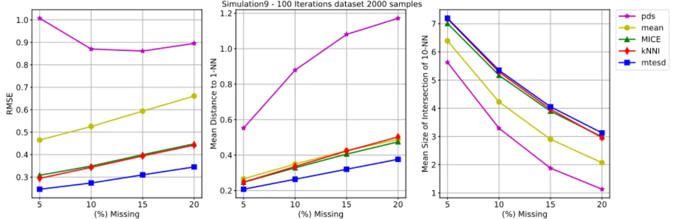
This dataset were built with a mixture of 3 components, each one having 3 components from the Normal distribution and 2 following the Multinomial distribution. We can see a clear advantage of the model estimation over the alternatives.
5 10 15 20 (%) Missing 0.3 0.4 0.5 0.6 0.7 0.8 0.9 1.0 RMSE 5 10 15 20 (%) Missing 0.2 0.4 0.6 0.8 1.0 1.2 Mean Distance to 1-NN
Simulation9 - 100 Iterations dataset 2000 samples
5 10 15 20 (%) Missing 1 2 3 4 5 6 7
Mean Size of Intersection of 10-NN
pds mean MICE kNNI mtesd
Figure 2 – Example 1: Normal-Bernoulli Mixture
Figure 2 shows the 95% confidence interval, with the empirical distribution of the sample, for the mean values of the evaluation criteria in the previous plot. Here, pds and
mean imputation were removed to make easier visualization. Tables 1, 2 and 3 shows the
values for the figures 1 and 2. The bold faced values are the winners, for easier visualization. The following datasets presentation follows the same scheme above.
Chapter 4. Results 30 5 10 15 20 (%) Missing 0.25 0.30 0.35 0.40 0.45 RMSE 5 10 15 20 (%) Missing 0.25 0.30 0.35 0.40 0.45 Mean Distance to 1-NN 95% Confidence interval 5 10 15 20 (%) Missing 3 4 5 6 7 8
Mean Size of Intersection of 10-NN
MICE knni mtesd ic(95%)
Figure 3 – Confidence Interval: Normal-Bernoulli Mixture
mis(%) MICE knni mean mtesd pds
mean std mean std mean std mean std mean std 5 0.3081 0.0275 0.2944 0.0824 0.4650 0.0463 0.2459 0.0169 1.0071 0.0260 10 0.3491 0.0331 0.3433 0.0950 0.5252 0.0589 0.2736 0.0171 0.8703 0.0365 15 0.3997 0.0445 0.3940 0.0969 0.5937 0.0705 0.3099 0.0157 0.8611 0.0529 20 0.4479 0.0607 0.4424 0.1140 0.6607 0.0883 0.3452 0.0143 0.8952 0.0724
Table 1 – RMSE statistics for Normal-Multinomial estimated distances.
mis(%) MICE knni mean mtesd pds
mean std mean std mean std mean std mean std 5 0.2469 0.0093 0.2474 0.0120 0.2664 0.0095 0.2075 0.0048 0.5521 0.1178 10 0.3281 0.0162 0.3353 0.0199 0.3494 0.0164 0.2638 0.0071 0.8791 0.2729 15 0.4056 0.0228 0.4230 0.0259 0.4252 0.0204 0.3201 0.0101 1.0808 0.3376 20 0.4748 0.0285 0.5026 0.0328 0.4885 0.0232 0.3762 0.0103 1.1717 0.3530
Table 2 – AvgNN statistics for Normal-Multinomial estimated distances.
mis(%) MICE knni mean mtesd pds
mean std mean std mean std mean std mean std 5 7.0065 0.1159 7.1760 0.1596 6.3929 0.1217 7.1921 0.1103 5.6289 0.3583 10 5.1688 0.1333 5.2860 0.3080 4.2262 0.1369 5.3474 0.1451 3.2923 0.5526 15 3.8958 0.1297 3.9658 0.3237 2.9009 0.1104 4.0533 0.1511 1.8768 0.6548 20 2.9903 0.1220 2.9617 0.3743 2.0690 0.0876 3.1270 0.1535 1.1307 0.6315
Table 3 – Avg10NN statistics for Normal-Multinomial estimated distances.
4.1.2
Normal-Poisson
Figures 3 and 4 shows the results from the Normal - Poisson mixture model. A very similar plot of the Figure 3was obtained in this simulation. Again, the model shows some advantage against its competitors in RMSE and average NN. Moreover, despite of
Chapter 4. Results 31
the lower accuracy in the third plot of Figure 3 of the mtesd, its confidence interval shows a reasonable approximation to the other models.
5 10 15 20 (%) Missing 1 2 3 4 5 RMSE 5 10 15 20 (%) Missing 1.0 1.5 2.0 2.5 3.0 3.5 Mean Distance to 1-NN
Simulation2 - 100 Iterations dataset 2000 samples
5 10 15 20 (%) Missing 2 3 4 5 6 7
Mean Size of Intersection of 10-NN
pds mean MICE kNNI mtesd
Figure 4 – Example 2: Normal - Poisson mixture
5 10 15 20 (%) Missing 1.0 1.2 1.4 1.6 1.8 2.0 RMSE 5 10 15 20 (%) Missing 0.8 1.0 1.2 1.4 1.6 1.8 Mean Distance to 1-NN 95% Confidence interval 5 10 15 20 (%) Missing 3 4 5 6 7 8
Mean Size of Intersection of 10-NN
MICE knni mtesd ic(95%)
Figure 5 – Confidence Interval: Normal - Poisson mixture
mis(%) MICE knni mean mtesd pds
mean std mean std mean std mean std mean std 5 1.3243 0.2259 1.3236 0.5734 2.4136 0.5428 0.9312 0.0837 5.3495 0.2527 10 1.5012 0.2472 1.5686 0.6459 2.6818 0.6101 1.0275 0.1093 4.5405 0.3210 15 1.7000 0.3064 1.7126 0.6315 2.8922 0.6988 1.1815 0.1389 4.4294 0.4018 20 1.9049 0.3631 1.9567 0.6983 3.1887 0.7512 1.3142 0.1670 4.5424 0.5326
Table 4 – RMSE statistics for Normal - Poisson estimated distances.
mis(%) MICE knni mean mtesd pds
5 1.0009 0.0564 0.9945 0.0700 1.0337 0.0629 0.8296 0.0163 1.8432 0.4372 10 1.2669 0.1211 1.3024 0.1339 1.2741 0.1080 0.9723 0.0372 2.7612 0.9137 15 1.4969 0.1493 1.5675 0.1600 1.4793 0.1323 1.1180 0.0543 3.3421 1.1648 20 1.7242 0.2090 1.8525 0.1963 1.6693 0.1792 1.2749 0.0843 3.7963 1.3994
Chapter 4. Results 32
mis(%) MICE knni mean mtesd pds
mean std mean std mean std mean std mean std 5 7.4440 0.2210 7.5694 0.2451 7.0940 0.2595 7.4191 0.1009 4.7678 0.1427 10 5.6836 0.3685 5.8431 0.4667 5.1814 0.3931 5.5387 0.1686 3.4507 0.2285 15 4.4428 0.3435 4.5673 0.4684 3.8777 0.3432 4.2017 0.1451 2.4644 0.2806 20 3.4744 0.3739 3.5354 0.4849 2.9682 0.3281 3.2018 0.1370 1.7343 0.3725
Table 6 – Avg10NN statistics for Normal - Poisson estimated distances.
4.1.3
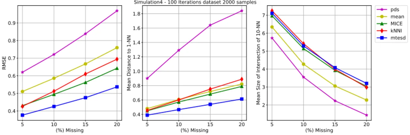
Normal - Multinomial - Exponential
Another example, with further mixing in the data distributions. The mixture was composed by a three component with 3 normals, 1 multinomial (Bernoulli) and 2 exponentials. 5 10 15 20 (%) Missing 0.4 0.5 0.6 0.7 0.8 0.9 RMSE 5 10 15 20 (%) Missing 0.4 0.6 0.8 1.0 1.2 1.4 1.6 1.8 Mean Distance to 1-NN
Simulation4 - 100 Iterations dataset 2000 samples
5 10 15 20 (%) Missing 2 3 4 5 6 7
Mean Size of Intersection of 10-NN
pds mean MICE kNNI mtesd
Figure 6 – Example 3: Normal - Multinomial - Exponential
5 10 15 20 (%) Missing 0.35 0.40 0.45 0.50 0.55 0.60 0.65 0.70 RMSE 5 10 15 20 (%) Missing 0.4 0.5 0.6 0.7 0.8 0.9 Mean Distance to 1-NN 95% Confidence interval 5 10 15 20 (%) Missing 3 4 5 6 7 8
Mean Size of Intersection of 10-NN
MICE knni mtesd ic(95%)
Chapter 4. Results 33
mis(%) MICE knni mean mtesd pds
mean std mean std mean std mean std mean std 5 0.4305 0.0677 0.4264 0.0752 0.5107 0.0617 0.3765 0.0658 0.6202 0.0554 10 0.4943 0.0616 0.5123 0.0776 0.5860 0.0576 0.4257 0.0618 0.7214 0.0527 15 0.5622 0.0553 0.6102 0.0908 0.6674 0.0541 0.4755 0.0526 0.8386 0.0480 20 0.6427 0.0579 0.6942 0.0809 0.7596 0.0567 0.5370 0.0580 0.9691 0.0517
Table 7 – RMSE statistics for Normal - Multinomial - Exponential estimated distances.
mis(%) MICE knni mean mtesd pds
mean std mean std mean std mean std mean std 5 0.4497 0.0168 0.4542 0.0200 0.4803 0.0171 0.3897 0.0087 0.9000 0.0917 10 0.5715 0.0280 0.6005 0.0292 0.6069 0.0283 0.4663 0.0153 1.2913 0.2085 15 0.6816 0.0320 0.7514 0.0301 0.7182 0.0317 0.5393 0.0183 1.6412 0.3960 20 0.7888 0.0371 0.8887 0.0310 0.8216 0.0348 0.6134 0.0215 1.8403 0.4204
Table 8 – AvgNN statistics for Normal - Multinomial - Exponential estimated distances.
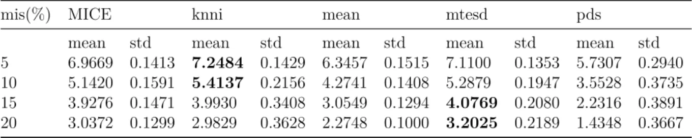
mis(%) MICE knni mean mtesd pds
mean std mean std mean std mean std mean std 5 6.9669 0.1413 7.2484 0.1429 6.3457 0.1515 7.1100 0.1353 5.7307 0.2940 10 5.1420 0.1591 5.4137 0.2156 4.2741 0.1408 5.2879 0.1947 3.5528 0.3735 15 3.9276 0.1471 3.9930 0.3408 3.0549 0.1294 4.0769 0.2080 2.2316 0.3891 20 3.0372 0.1299 2.9829 0.3628 2.2748 0.1000 3.2025 0.2189 1.4348 0.3667
Table 9 – Avg10NN statistics for Normal - Multinomial - Exponential estimated distances.
4.1.4
Multinomial
This is an instance that may illustrate how flexible and efficient this methodology can be, running the model over completely discrete/categorical data. A good improvement in the RMSE followed by some small gain over NN prediction.
5 10 15 20 (%) Missing 0.8 1.0 1.2 1.4 1.6 RMSE 5 10 15 20 (%) Missing 0.2 0.4 0.6 0.8 1.0 1.2 Mean Distance to 1-NN
Simulation8 - 100 Iterations dataset 2000 samples
5 10 15 20 (%) Missing 1.0 1.5 2.0 2.5 3.0
Mean Size of Intersection of 10-NN
pds mean MICE knni mtesd
Chapter 4. Results 34 5 10 15 20 (%) Missing 0.7 0.8 0.9 1.0 1.1 1.2 RMSE 5 10 15 20 (%) Missing 0.1 0.2 0.3 0.4 0.5 Mean Distance to 1-NN 95% Confidence interval 5 10 15 20 (%) Missing 1.5 2.0 2.5 3.0 3.5
Mean Size of Intersection of 10-NN
MICE knni mtesd ic(95%)
Figure 9 – Confidence Interval: Multinomial Mixture
mis(%) MICE knni mean mtesd pds
mean std mean std mean std mean std mean std 5 0.7961 0.0260 0.7852 0.0240 0.7906 0.0241 0.6508 0.0139 1.5888 0.0277 10 0.9213 0.0297 0.9024 0.0262 0.8959 0.0257 0.7190 0.0148 1.3164 0.0292 15 1.0510 0.0362 1.0270 0.0316 0.9908 0.0290 0.7907 0.0173 1.2585 0.0383 20 1.1829 0.0400 1.1500 0.0360 1.0726 0.0296 0.8567 0.0166 1.2733 0.0509
Table 10 – RMSE statistics for Multinomial estimated distances.
mis(%) MICE knni mean mtesd pds
mean std mean std mean std mean std mean std 5 0.1378 0.0110 0.1456 0.0174 0.1402 0.0118 0.1123 0.0102 0.4500 0.1017 10 0.2742 0.0173 0.2899 0.0253 0.2736 0.0181 0.2234 0.0161 0.7972 0.1200 15 0.4124 0.0242 0.4316 0.0288 0.4078 0.0242 0.3931 0.0390 1.1086 0.1575 20 0.5497 0.0334 0.5629 0.0324 0.5374 0.0292 0.5291 0.0515 1.3359 0.1436
Table 11 – AvgNN statistics for Multinomial estimated distances.
mis(%) MICE knni mean mtesd pds
mean std mean std mean std mean std mean std 5 3.0398 0.1868 3.0275 0.2050 2.9752 0.1833 3.0786 0.1903 2.2408 0.1618 10 2.4089 0.1330 2.3774 0.1405 2.2705 0.1248 2.4430 0.1453 1.4351 0.1396 15 1.9312 0.0992 1.8787 0.0842 1.7765 0.0769 1.9518 0.1001 0.9683 0.1072 20 1.5582 0.0939 1.5013 0.0796 1.4101 0.0638 1.5639 0.1071 0.6740 0.0870
Table 12 – Avg10NN statistics for Multinomial estimated distances.
4.2
Real Data
These datasets were obtained from sources on the UCI Machine Learning Repository (DHEERU; TANISKIDOU,2017) and have in common the presence of multivariate mixed
Chapter 4. Results 35
4.2.1
Wine dataset
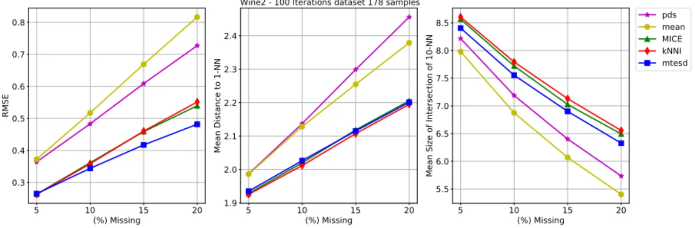
The Wine dataset is a classic in machine learning studies. It is a tabular dataset that contains 14 features and 178 observations, where all but the first column (Class) were used. For further details about this dataset, check (CORTEZ et al.,2009).
5 10 15 20 (%) Missing 0.3 0.4 0.5 0.6 0.7 0.8 RMSE 5 10 15 20 (%) Missing 1.9 2.0 2.1 2.2 2.3 2.4 Mean Distance to 1-NN
Wine2 - 100 Iterations dataset 178 samples
5 10 15 20 (%) Missing 5.5 6.0 6.5 7.0 7.5 8.0 8.5
Mean Size of Intersection of 10-NN
pds mean MICE kNNI mtesd
Figure 10 – Example 6: Wine dataset results
5 10 15 20 (%) Missing 0.25 0.30 0.35 0.40 0.45 0.50 0.55 RMSE 5 10 15 20 (%) Missing 1.90 1.95 2.00 2.05 2.10 2.15 2.20 2.25 2.30 Mean Distance to 1-NN 95% Confidence interval 5 10 15 20 (%) Missing 5 6 7 8 9
Mean Size of Intersection of 10-NN
MICE knni mtesd ic(95%)
Figure 11 – Confidence Interval: Wine dataset
mis(%) MICE knni mean mtesd pds
mean std mean std mean std mean std mean std 5 0.2634 0.0341 0.2628 0.0349 0.3725 0.0307 0.2651 0.0324 0.3643 0.0257 10 0.3618 0.0348 0.3585 0.0367 0.5173 0.0337 0.3442 0.0331 0.4833 0.0293 15 0.4588 0.0367 0.4604 0.0347 0.6690 0.0345 0.4173 0.0347 0.6088 0.0302 20 0.5396 0.0331 0.5515 0.0349 0.8165 0.0330 0.4818 0.0348 0.7273 0.0305
Chapter 4. Results 36
mis(%) MICE knni mean mtesd pds
mean std mean std mean std mean std mean std 5 1.9282 0.0212 1.9254 0.0204 1.9859 0.0255 1.9348 0.0187 1.9865 0.0318 10 2.0198 0.0313 2.0117 0.0361 2.1284 0.0475 2.0264 0.0298 2.1371 0.0489 15 2.1184 0.0413 2.1072 0.0387 2.2548 0.0513 2.1152 0.0387 2.2989 0.0562 20 2.2054 0.0481 2.1948 0.0470 2.3790 0.0590 2.2011 0.0436 2.4561 0.0701
Table 14 – AvgNN statistics for Wine dataset.
mis(%) MICE knni mean mtesd pds
mean std mean std mean std mean std mean std 5 8.5633 0.1814 8.6043 0.1690 7.9794 0.1924 8.4053 0.1691 8.2163 0.1748 10 7.7211 0.1895 7.7931 0.2088 6.8742 0.2266 7.5532 0.1857 7.1884 0.1987 15 7.0258 0.2014 7.1312 0.1842 6.0698 0.2087 6.9012 0.1985 6.4020 0.1867 20 6.4928 0.1747 6.5546 0.2001 5.4026 0.2168 6.3276 0.1885 5.7345 0.1797
Table 15 – Avg10NN statistics for Wine dataset
4.2.2
COIL dataset
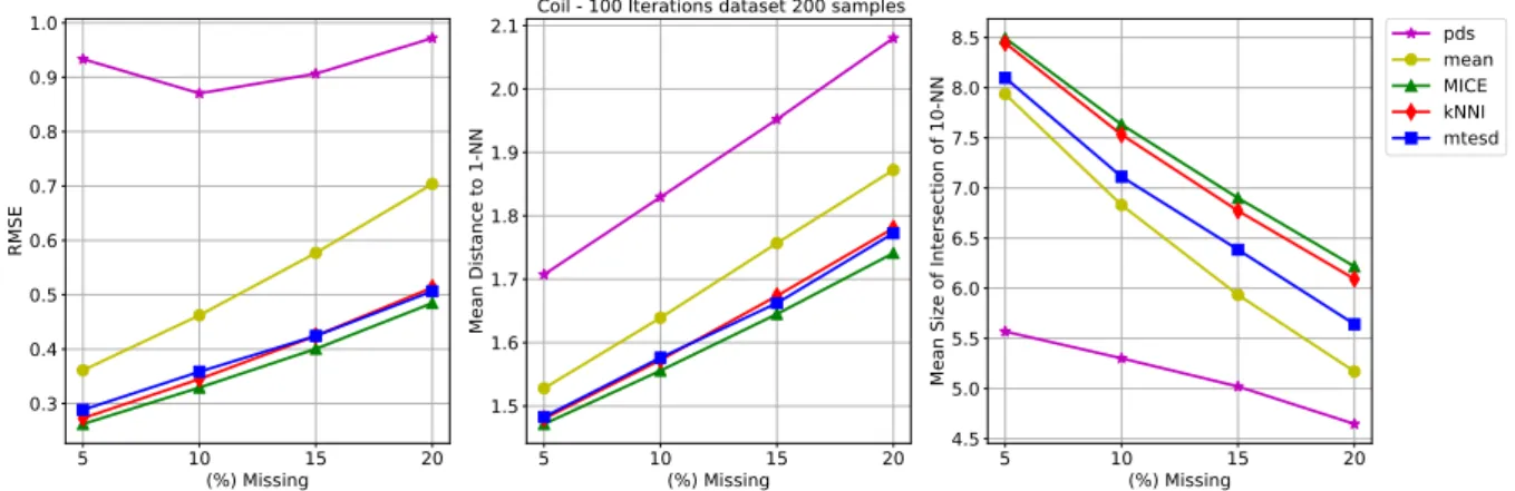
The COIL 1999 competition dataset is an example of mixed data type. It is a tabular dataset that contains 18 features and 200 observations, where all but the columns 11 and 18 were used. For further details about this dataset, check (DHEERU; TANISKIDOU,
2017). 5 10 15 20 (%) Missing 0.3 0.4 0.5 0.6 0.7 0.8 0.9 1.0 RMSE 5 10 15 20 (%) Missing 1.5 1.6 1.7 1.8 1.9 2.0 2.1 Mean Distance to 1-NN
Coil - 100 Iterations dataset 200 samples
5 10 15 20 (%) Missing 4.5 5.0 5.5 6.0 6.5 7.0 7.5 8.0 8.5
Mean Size of Intersection of 10-NN
pds mean MICE kNNI mtesd
Chapter 4. Results 37 5 10 15 20 (%) Missing 0.25 0.30 0.35 0.40 0.45 0.50 RMSE 5 10 15 20 (%) Missing 1.5 1.6 1.7 1.8 Mean Distance to 1-NN 95% Confidence interval 5 10 15 20 (%) Missing 4 5 6 7 8 9
Mean Size of Intersection of 10-NN
MICE knni mtesd ic(95%)
Figure 13 – Confidence Interval: coil dataset
mis(%) MICE knni mean mtesd pds
mean std mean std mean std mean std mean std 5 0.2623 0.0386 0.2730 0.0395 0.3611 0.0411 0.2883 0.0326 0.9333 0.0298 10 0.3293 0.0331 0.3450 0.0331 0.4622 0.0374 0.3584 0.0281 0.8703 0.0240 15 0.4006 0.0327 0.4245 0.0374 0.5769 0.0417 0.4244 0.0278 0.9065 0.0236 20 0.4847 0.0384 0.5131 0.0437 0.7037 0.0460 0.5064 0.0313 0.9719 0.0314
Table 16 – RMSE statistics for Coil dataset.
mis(%) MICE knni mean mtesd pds
mean std mean std mean std mean std mean std 5 1.4716 0.0308 1.4800 0.0332 1.5280 0.0371 1.4829 0.0234 1.7073 0.0453 10 1.5558 0.0375 1.5725 0.0409 1.6391 0.0467 1.5762 0.0316 1.8295 0.0548 15 1.6451 0.0447 1.6737 0.0462 1.7568 0.0526 1.6623 0.0405 1.9521 0.0727 20 1.7411 0.0596 1.7804 0.0661 1.8722 0.0596 1.7726 0.0620 2.0802 0.0918
Table 17 – AvgNN statistics for Coil dataset.
mis(%) MICE knni mean mtesd pds
mean std mean std mean std mean std mean std 5 8.4944 0.2315 8.4446 0.2276 7.9367 0.2597 8.0989 0.1939 5.5686 0.1283 10 7.6323 0.2247 7.5312 0.2310 6.8299 0.2494 7.1122 0.2192 5.3012 0.1454 15 6.8999 0.2460 6.7720 0.2598 5.9341 0.2538 6.3845 0.2349 5.0205 0.1817 20 6.2167 0.2935 6.0926 0.3103 5.1701 0.2898 5.6412 0.2933 4.6465 0.2377
Table 18 – Avg10NN statistics for Coil dataset
4.2.3
Abalone dataset
The Abalone dataset was generated in a study of mixed data type. It is a tabular dataset that contains 9 features and 4000 observations, where all but the last one, the estimated age, were used. For further details about this dataset, check (NASH et al.,1994).
Chapter 4. Results 38 5 10 15 20 (%) Missing 0.2 0.3 0.4 0.5 0.6 0.7 0.8 0.9 RMSE 5 10 15 20 (%) Missing 0.3 0.4 0.5 0.6 0.7 Mean Distance to 1-NN
Abalone - 100 Iterations dataset 4177 samples
5 10 15 20 (%) Missing 2 3 4 5 6 7 8
Mean Size of Intersection of 10-NN
pds mean MICE kNNI mtesd
Figure 14 – Example 8: Abalone dataset
5 10 15 20 (%) Missing 0.2 0.3 0.4 0.5 0.6 0.7 RMSE 5 10 15 20 (%) Missing 0.275 0.300 0.325 0.350 0.375 0.400 0.425 0.450 Mean Distance to 1-NN 95% Confidence interval 5 10 15 20 (%) Missing 3 4 5 6 7 8
Mean Size of Intersection of 10-NN
MICE knni mtesd ic(95%)
Figure 15 – Confidence Interval: Abalone dataset
mis(%) MICE knni mean mtesd pds
5 0.2017 0.2846 0.2256 0.2847 0.4283 0.2382 0.3081 0.2617 0.6435 0.2121 10 0.3364 0.3639 0.3735 0.3610 0.5980 0.2788 0.4436 0.3282 0.7459 0.2514 15 0.4670 0.4153 0.5013 0.3593 0.7428 0.2634 0.5496 0.3337 0.8674 0.2418 20 0.4754 0.3606 0.5698 0.3454 0.8344 0.2419 0.5843 0.3201 0.9454 0.2122
Table 19 – RMSE statistics for Abalone dataset.
mis(%) MICE knni mean mtesd pds
mean std mean std mean std mean std mean std 5 0.2621 0.0053 0.2646 0.0068 0.3185 0.0076 0.2726 0.0059 0.3752 0.0087 10 0.3150 0.0127 0.3229 0.0144 0.4002 0.0156 0.3297 0.0100 0.5081 0.0230 15 0.3684 0.0150 0.3882 0.0193 0.4716 0.0188 0.3832 0.0111 0.6405 0.0518 20 0.4199 0.0171 0.4577 0.0296 0.5362 0.0241 0.4335 0.0132 0.7702 0.0902
Chapter 4. Results 39
mis(%) MICE knni mean mtesd pds
mean std mean std mean std mean std mean std 5 7.8388 0.0954 7.8352 0.1107 5.5295 0.1723 6.5068 0.1479 6.9074 0.1738 10 6.3822 0.2217 6.3268 0.2467 3.2893 0.1902 4.7122 0.2004 5.0589 0.2542 15 5.2595 0.1988 5.0862 0.2756 2.1296 0.1453 3.6935 0.2008 3.7694 0.2805 20 4.3102 0.2349 3.9943 0.3584 1.4779 0.1149 2.9201 0.2018 2.7839 0.2940
40
5 Discussion
The results for the synthetic datasets shows the trained model have a good fit for all the evaluation criteria. In the continuous/categorical parts of the first two synthetic datasets, the execution time measurements were very short in comparison with some of the purely categorical and real datasets, like Abalone. Some part of it is due to the model selection time when the model must run multiple times to perform a step like a cross-validation/regularization, in the machine learning point of view. Although it may poses some limitation in the computational costs, mixture models is a model completely apart from the objective of distance estimation, so it can be very useful in obtaining more insights and statistical properties not assessed by traditional imputation methods. The choice of the composed distance 3.3in this methodology gave good results, showing great improvement over the traditional L2-norm estimation for the mixed-type mixtures. The confidence intervals of mtesd always covered the mean results of other models in the synthetic datasets, when it did not performed better with good advantage like in the Normal - Multinomial and Normal - Poisson models.
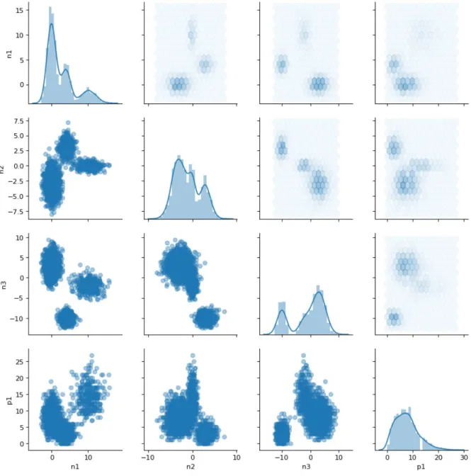
In the real datasets, some improvements in the estimation process were obtained, like ’standardization’ of the information, in a sense that continuous data should be scaled and translated according to their respective chosen distributions, and categorical data should be transformed in the right domain to make the expected computations, e.g.: {0, 3, 5, 7} converts to {0, 1, 2, 3}. Given some plots, like figure 16, some insights about data distribution can be obtained. In cases like Abalone and Coil datasets, transformations like logarithm were performed to give the data some similarity with the Normal (Gaussian) distribution, having the mixture adjusted by mtesd. Despite of the better results in Coil and Wine, the mtesd results in Abalone and previously expected results on other data indicates that some relations in this data must be better examined. This case is the result on the use of AICcmodel selection criterium, whose construction restricted the number of components in the mixture, for all the simulation runs, to be 1. This example is good to notice some robustness of the model of distance estimation even if a not well suited model selection were done in the mixture estimation step.
Chapter 5. Discussion 41
Chapter 5. Discussion 42
Figure 17 – Scatter Matrix: Coil dataset
This methodology avoided the use of complete covariance matrices, focusing only in the variances, the diagonal of the matrix, and the results shown above make clear the good fitting that mixtures with local independence can obtain, avoiding the higher complexity computations of the traditional GMM.
43
6 Conclusion
Mixture estimation to compute distance works well in many cases where GMM may fail due to the dataset nature. Given the extra resources, which are not also present in any other models, but can be obtained from the mixture models, one can make further estimations with some non-usual distance metrics. This suggests further works with estimation of distances with another metrics.
The exponential family, as mentioned before in the section 3.3, make easier to obtain the sufficient statistics of the target parameters for each distribution and have made this proposal with mixed-type mixtures a very interesting approach, raising some other questions and proposals for future works, like GLM estimation. Some tests with stochastic gradient descents and better initialization of the EM algorithm could be done, in order to have a better performance and less execution time. Evaluation of some machine learning algorithms, coupled with the distance estimation performed by mtesd and tests against the GMM-based imputation are also a natural path to follow in order to establish the real improvements of this work proposed methodology in the bigger scenario of machine learning with incomplete data. A better programming design of mtesd can lead to very competitive tool with good evaluation time in the small to mid sized datasets, looking at regular, tabular shaped data with less than 5000 instances and from 10 to 20 columns took around 2 seconds on a machine with eight threaded CPU, without much optimization in the code written in Python. This methodology certainly deserves further attention due to its generalization aspects and connections to many useful problems in the machine learning and data science fields.
44
References
BROWNE, R. P. et al. Model-based clustering, classification, and discriminant analysis of data with mixed type. [S.l.]: Journal of Statistical Planning and Inference, 2012. Citado na página 17.
BUUREN, S. V. et al. Flexible Multivariate Imputation by MICE. 1999. Citado 2 vezes nas páginas 15and 28.
CORTEZ, P. et al. Modeling wine preferences by data mining from physicochemical properties. Decision Support Systems, Elsevier, v. 47, n. 4, p. 547–553, 2009. Citado na página 35.
COTTRELL, M. et al. Missing values: processing with the kohonen algorithm. arXiv
preprint math/0701152, 2007. Citado na página 16.
DELALLEAU, O. et al. Efficient em training of gaussian mixtures with missing data.
arXiv preprint arXiv:1209.0521, 2012. Citado na página 16.
DEMPSTER, A. P. et al. Maximum likelihood from incomplete data via the em algorithm. Journal of the royal statistical society. Series B (methodological), JSTOR, p. 1–38, 1977. Citado 2 vezes nas páginas13and 23.
DHEERU, D. et al. UCI Machine Learning Repository. 2017. Disponível em: <http: //archive.ics.uci.edu/ml>. Citado 2 vezes nas páginas 34and 36.
DIXON, J. K. Pattern recognition with partly missing data. IEEE Transactions on Systems, Man, and Cybernetics, IEEE, v. 9, n. 10, p. 617–621, 1979. Citado 2 vezes nas páginas 15 and 28.
DOQUIRE, G. et al. Feature selection with missing data using mutual
informa-tion estimators. 2012. Citado na página 15.
EIROLA, E. et al. Distance estimation in numerical data sets with missing values. [S.l.]: Information Sciences, 2013. Citado 3 vezes nas páginas 15, 16, and17.
. Mixture of Gaussians for distance estimation with missing data. [S.l.]: Neurocomputing, 2013. Citado na página 16.
FARHANGFAR, A. et al. Impact of imputations of missing values on classification
error for discrete data. [S.l.]: Pattern Recognition 41, 2008. Citado na página 15.
GHAHRAMANI, Z. et al. Supervised learning from incomplete data via an EM
approach. [S.l.]: Morgan Kaufmann Publishers, 1994. Citado na página 16.
GOODMAN, L. A. Exploratory latent structure analysis using both identifiable and unidentifiable models. Biometrika, Oxford University Press, v. 61, n. 2, p. 215–231, 1974. Citado na página 23.
JORGENSEN, M. A. et al. Mixture Model Clustering of Data Sets with Cate-gorical and Continuous Variables. [S.l.]: Proceedings of the Conference ISIS, 1996. Citado 2 vezes nas páginas 17 and 23.
References 45
LAZARSFELD, P. F. et al. Latent structure analysis. [S.l.]: Houghton Mifflin Company, Boston, Massachusetts, 1968. Citado na página 23.
LITTLE, R. J. A. et al. Statistical Analysis with Missing Data. 2nd ed. ed. [S.l.]: Wiley Interscience, 2002. Citado 2 vezes nas páginas15 and 20.
MACLACHLAN, G. et al. Finite Mixture Models. [S.l.]: John Wiley and Sons, 2004. Citado na página 22.
MCLACHLAN, G. J. et al. The EM Algorithm and Extensions. [S.l.]: John Wiley & Sons, 2008. Citado na página 23.
NASH, W. J. et al. The population biology of abalone (haliotis species) in tasmania. i. blacklip abalone (h. rubra) from the north coast and islands of bass strait. Sea Fisheries
Division, Technical Report, n. 48, 1994. Citado na página 37.
OLIPHANT, T. E. A guide to NumPy. [S.l.: s.n.], 2006. v. 1. Citado na página 28. PAULA, G. A. Modelos de Regressão com apoio computacional. [S.l.: s.n.], 2013. Citado na página 23.
STEELE, R. J. et al. Inference from multiple imputation for missing data using mixtures of normals. Statistical methodology, Elsevier, v. 7, n. 3, p. 351–365, 2010. Citado na página 16.
TRESP, V. et al. Training neural networks with deficient data. In: Advances in neural
information processing systems. [S.l.: s.n.], 1994. p. 128–135. Citado na página 16.
TROYANSKAYA, O. et al. Missing value estimation methods for dna microarrays.
Bioin-formatics, Oxford University Press, v. 17, n. 6, p. 520–525, 2001. Citado na página