DGPS based methods to obtain beach cusp dimensions

DGPS based methods to obtain beach cusp dimensions 541

DGPS based methods to obtain beach cusp dimensions.

Vítor Lopes†, Paulo Baptista‡, Joaquim Pais-Barbosa†, Francisco Taveira-Pinto†, Fernando Veloso-Gomes† † Faculdade de Engenharia da

Universidade do Porto, R. Dr. Roberto Frias, s/n, 4200-007, Portugal. vitor.oliveira.lopes@fe.up.pt jlpb@fe.up.pt

fpinto@fe.up.pt

vgomes@fe.up.pt

‡ Departamento de Geociências, Centro de Estudos do Ambiente e do Mar (CESAM), Universidade de Aveiro, Campus Universitário de Santiago, 3810-193 Aveiro, Portugal

renato.baganha@ua.pt

INTRODUCTION

A beach cusp is defined as a cuspate feature which usually occurs in groups along the foreshore as a series of alternating horns (pointing seaward) and embayments (such a series usually being called a beach cusp system).

Many attempts have been made in order to correlate measured beach cusp spacing to wave conditions (Aoki and Sunamura, 2000; Pais-Barbosa, 2007) or to values of spacing given by theoretical expressions (Holland and Holman, 1996; Holland, 1998, Masselink, 1999) associated to standing edge wave theory or to self-organization theory. If we want to correlate cusp dimensions to determined wave parameters we should have a large data set (preferably referring to the same site) in order to obtain significant statistical relations.

Coco et al. (1999) performed an extensive search of relevant literature regarding beach cusps and collected 92 cusp spacing values, as well as wave parameters referring to those spacings. Lopes et al. (2011) used Coco et al. (1999) data and applied multivariate data analysis techniques to it in order to study the correlation between beach cusp spacing and several wave parameters in an attempt to assess which one would better correlate to cusp spacing. When dealing with multivariate data analysis problems the need for a large data set is even greater.

There are many papers providing field measurements of beach cusp spacing (Takeda and Sunamura, 1983; Rasch et al., 1993 among many others). The same cannot be said for other beach cusp dimensions such as cusp depth, height or elevation. As far as

the authors are aware, only Nolan et al. (1999) and more recently van Gaalen et al. (2011), provide measurements of all of the above-mentioned dimensions simultaneously. However Nolan’s work refers to multiple sites and van Gaalen’s work refers to a five-day period only. Coco et al. (2004) provide measurements for height but not for spacing or depth. Correlations between different wave parameters and cusp dimensions other than spacing may provide higher correlations and as such provide better insight into what processes intervene in cusp formation and evolution. Moreover, relationships between cusp dimensions are of particular interest (Nolan et al., 1999).

Coco et al. (1999) point out that beach cusp research is in desperate need of three-dimensional observations of evolving cusp morphology (along with hydrodynamical measurements) to assess what role edge waves or self-organization mechanisms play in determining typical cusp length scales.

Different authors have used different methods to obtain beach cusp spacing. Masselink (1999) used an electronic survey station to derive cusp spacing and other parameters. Nolan et al. (1999) determines cusp spacing and depth with a tape measure while height and elevation were obtained from beach profile surveys. In Almar et al. (2008) spacing values were manually digitized from averaged video images. Vousdoukas (2012) examines a five-month period of coastal imagery to extract shoreline contours at a fixed elevation (1 and 3 m above mean sea level). The elevations of the automatically extracted contours were estimated as a function of offshore wave and tidal measurements. After verifying the existence of beach cusps, the locations of the cusp horns and embayments were manually identified from the contour positions. van Gaalen et al. (2011) uses terrestrial laser scanning and ABSTRACT

Lopes, V., Baptista, P., Pais-Barbosa, J., Taveira-Pinto, F., Veloso-Gomes, F., 2013. DGPS based methods to obtain beach cusp dimensions. In: Conley, D.C., Masselink, G., Russell, P.E. and O’Hare, T.J. (eds.), Proceedings 12th

International Coastal Symposium (Plymouth, England), Journal of Coastal Research, Special Issue No. 65, pp.

xxx-xxx, ISSN 0749-0208.

Statistical correlations between wave parameters and cusp dimensions other than spacing may provide insight into which processes intervene in beach cusps formation and evolution. However, there is little information about cusp dimensions such as cusp depth, height or elevation. The aim of this work is to evaluate and compare different methods to determine beach cusp dimensions in order to assess which one produces more accurate, extensive and easy-to-achieve results. For this purpose some beach surveys were carried out at Ofir beach, located on the Portuguese west coast. Each one of the methods uses different sampling and processing strategies to obtain beach cusp dimensions. In method 0 cusp dimensions were determined using only two tape measures. The remaining 4 methods use Differential Global Positioning System (DGPS). Methods 3 and 4 provide values for cusp spacing, height, elevation and depth whilst methods 1 and 2 provide values for the first three parameters only. If one is only interested in measuring beach cusp spacing, height and elevation, then method 1 seems to be more adequate, due to its ease in sampling and in dealing with the data processing. Values of spacing, height and elevation obtained via Method 1 are the most accurate ones. On the other hand, if one wishes to perform a more detailed analysis, including parameters other than the above-mentioned and, for instance, to produce Digital Elevation Models (DEM), a combination of Method 1 and Method 3 or 4 is more appropriate.

ADDITIONAL INDEX WORDS: beach surveys, sampling strategies, processing strategies, statistical correlations

www.cerf-jcr.org

____________________

DOI: 10.2112/SI65-092.1 received 07 December 2012; accepted 06 March 2013.

542 Lopes, et al.

sediment analysis to study beach cusp morphodynamics at Melbourne Beach (Florida, USA). With this technology, beach surveys in excess of hundreds of meters with sub-centimeter or even sub-millimeter spatial resolution can be completed during the course of a few hours. Surveys were run ~500 m alongshore and cusps dimensions were all gathered from DEMs created from the survey data. An S Transform was used to calculate cusp spacing. In Holland and Holman (1996) measurements of foreshore topography were taken for a week using vehicles equipped with Global Positioning System (GPS) surveying instrumentation. Beach topography was sampled daily to a vertical accuracy of better than 2 cm. Survey points were densely spaced (approximately every 3 m) within a 400 m longshore by 50 m cross-shore region. To reduce subjectivity in cusp length measurements, they calculated average (alongshore) cusp spacing from the wavenumber (reciprocal wavelength) spectrum of the alongshore variation in horizontal position of the measured 1 m elevation contour. Benavente et al. (2011) used RTK-GNSS (Real Time Kinematic Global Navigation Satellite System) to obtain alongshore profiles made through the cusp system. Cusp spacing values were calculated from these alongshore profiles.

For the purpose of correlating cusp dimensions with wave parameters there is a need for a large set of cusp dimension values (not only spacing, but also elevation, height and depth) referring to a single site. If we want to obtain measurements of a large set of beach cusp forming events we should have a fast means of

sampling data and obtaining cusp dimensions once the data is sampled (e.g., we should, ideally, use an automated processing method of obtaining cusp spacing and/or other cusp dimensions). The aim of this work is to propose/test different methods for determining beach cusp dimensions and to compare them in order to assess which one produces more accurate and easy-to-achieve results.

Each one of the methods uses different sampling and processing strategies to obtain cusp dimensions. Cusp dimensions in methods 1 and 2 are obtained in an almost automated way (through a set of Matlab scripts) whereas in methods 3 and 4 AutoCAD is used to extract them from digital elevation models.

METHODS

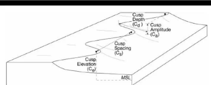
The regular cusp geometry frequently depicted in simplified schemes present in the literature (Figure 1) is not always seen in the field. Horn tips of a beach cusp system aren’t necessarily at the same elevation, nor located along the same straight line. The horns are not always parallel one to another and beach cusps are not always symmetric (Figure 2).

The definitions of cusp dimensions given by Nolan et al. (1999) are mentioned below, followed by a description of the slightly different definitions herein considered. First of all, it is convenient to define “horn tip”, which is the point of highest relief on a cusp horn. The above-mentioned author defines cusp elevation (Ce) as the highest point on the cusp horn above a datum. In the present work cusp elevation is defined as the mean value of the elevations of the two cusp “horn tips” that comprise a single beach cusp (elevations are taken relative to mean sea level at Cascais on 1938). Cusp spacing (Cs) is defined by Nolan et al. (1999) as the horizontal alongshore distance between the points of highest relief on two cusp horns. Herein cusp spacing is defined as the distance between two adjacent “horn tips”. The point situated along the line connecting two consecutive “horn tips” (here called the “connecting line”) which presents the lowest elevation value will be called the “lowest point”. The same author considers cusp amplitude (Ca) or cusp height as the maximum height difference (relief) of the cusp horn and the cusp bay. This measurement is taken from the highest point on the cusp horn (in a line parallel to the shoreline) to the lowest point in the cusp bay (Figure 1). In the Figure 1. Definition of beach cusp parameters (Nolan et al.,

1999).

DGPS based methods to obtain beach cusp dimensions 543

present work cusp height is defined as the difference between cusp elevation and the “lowest point” elevation. In Nolan et al. (1999) work cusp depth (Cd) is defined as the distance from the maximum high point on the cusp horn to the limit of swash excursion in the rear of the bay (Figure 1). However, Nolan et al. (1999) point out some problems in measuring cusp depth, namely the difficulty in determining it during high tide, when the seaward-most cusp relief was under water. Herein cusp depth is defined as the horizontal distance between the “lowest point” and the “back point” (Figure 2). The “back point” is the most landward point of the contour line defined by the mean elevation of the “horn tips”.

Five methods for determining beach cusp dimensions obtained from field surveys are now described. These methods differ from each other in terms of the way data is sampled and also in the way that cusp dimensions are extracted from the processed raw data. Method 0 is the only one that does not use GPS technology to collect the data. In the former method four operators are needed to collect the data. All the other methods only need one operator and are based on DGPS.

All surveys were conducted at Ofir beach, on the Portuguese west coast, near the Cávado river estuary, a highly energetic beach with semi-diurnal tide (maximum tidal range of 4 m). A total of four surveys were made, the first one in 12-03-2012, the second one in 19-03-2012 and the third and fourth in 08-06-2012. In each survey a set of 3 beach cusps was considered (approximately 100m*50m). A total of 12 measured beach cusps are discussed in this work. The surveys took place at time intervals close to low tide and during spring tides. Surveys 3 and 4 were done on the same day, one before low tide (survey 3) and the other one after (survey 4). While beach cusp were being surveyed a larger survey (of the entire Ofir beach) was carried out simultaneously using a mobile platform (four-wheel motor quad), and data from this survey was also analyzed. The set of grid points sampled with the mobile platform in the section where the cusps were being measured was no different (it had the same density) from all the other sections of Ofir beach that were covered by the four-wheel motor quad survey.

Method 0

Cusp spacing, height and depth were determined using only two tape measures. This method requires the participation of four elements. One person, positioned in one of the two “horn tips”, holds one end of the tape measure, and another person, positioned

on the second “horn tip”, holds the other end. A third person identifies the “lowest point” and positions himself there. This third person measures beach cusp height (distance from the soil to the tape measure connecting the two “horn tips”). In the sand, a fourth person draws the “mean contour” line that connects the two “horn tips” and identifies the “backpoint”. The third and fourth operators measure cusp depth. This method produces results for cusp spacing, height and depth. It should be noted that although the “horn tip” and the “lowest point” are normally easily identifiable there are exceptions to this. Also note that the “backpoint” is difficult to identify in the field.

Method 1

In this method the DGPS operator performs an on-foot survey with the GPS rover’s antenna mounted on a telescopic pole with a wheel on its lower end as described in Baptista et al., (2011a). The track covered by the operator is that which connects all the “horn tips” of the beach cusp system. The GPS acquisition mode is Stop and Go. The operator stops for approximately 30 seconds at the first “horn tip” of the system. When this time interval expires he walks along the line connecting the first “horn tip” to the second one and, when he reaches the lowest point of that line, stops again for 30 seconds. Once this second time interval is over, the operator continues all along the line and after finding the second “horn tip” of that connecting line, he again stops for 30 seconds. This process is repeated for all the “horn tip” connecting lines.

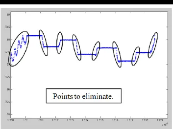
When it comes to cleaning up the data, a Matlab GUI (Cunha, 2002) is used to view the surveyed path and to eliminate superfluous data points. The data points are represented in a planimetric viewer (horizontal coordinate’s domain) as well as in the time versus elevation domain (Figure 3). The points of the track that are not relative to a “horn tip” or to a “lowest point” are easily identified and eliminated. The first and last values corresponding to the stopping periods are also eliminated. In this way, for each horn point and “lowest point” a set of approximately 30 values is obtained. These values are averaged and the coordinates of each “horn tip” and “lowest point” are obtained Afterwards, it is easy to calculate the spacing and the height of each cusp of the set (the height being taken as the difference between the mean elevation of the two “horn tips” and the elevation of the “lowest point”), as well as the mean spacing and mean height of the cusp system. This method only requires one person; it does not require spending a lot of time collecting the data; and being almost totally automated, it does not require much processing time. One shortcoming of this method is that it does not provide values for cusp depth.

Method 2

In this on-foot survey method the GPS works in kinematic mode and the operator walks along the same path as in method 1 but does not stop either at the “horn tip” or in the “lowest point”. In this way only a single triplet of x, y and z coordinates are sampled for each “horn tip” and “lowest point”. With the help of the Matlab GUI we simply clean up every point of the time versus ellipsoidal elevation curve, except the ones corresponding to the local maximums and minimums. The height and spacing are calculated in a similar way to method 1.

Note that the points inside the ellipse located on the left side of Figure 3 comprise the points of the time versus ellipsoidal elevation curve that are to be used in this method to extract local maximums and minimums.

Figure 3. Snapshot of the GUI used to clean up the data. Time (s) versus Ellipsoidal Elevations (m) domain.

544 Lopes, et al.

Method 3

In this method, which also uses the GPS in kinematic mode, the operator walks along several cross and longshore transects. Cross shore transects are made in a line more or less perpendicular to the coastline. Each cross shore transect includes one “horn tip” or “lowest” point.

The resulting data set, after interpolation in a 1*1 m grid, allows us to create a Digital Elevation Model (DEM). At this point the question arises of which contour line shall be chosen to extract cusp dimensions. The criteria used to choose it is somewhat subjective (we have no information about elevation of “horn tips” in this method and identifying them from 3D surfaces is not straightforward). We choose, by visual inspection, the contour line that appeared to present the most prominent curvature of the contour plot. The values of the interpolated DEM and of the coordinates of the chosen contour line (contained in matrix C produced by Matlab command contour) are then automatically exported to DXF AutoCad format. In the AutoCad environment the “horn tips”, the “lowest point” (one of the points of the interpolated grid is chosen) and the “back point” are identified and spacing, height and depth are measured.

Method 4

The most significant differences between method 3 and 4 reside in acquisition methodology. In method 4 the INSHORE system, which was designed for morphological survey of large sandy shore areas – 30 to 40 hectares per hour (Baptista et al., 2011b) uses a set of GPS antennas and a Distance Measurement Unit (DMU) mounted on a mobile platform (four-wheel motor quad). The track followed in method 4 is not as dense as the one followed in method 3 (there are fewer alongshore and especially cross-shore transects). Extraction of cusp dimensions from the DEM is done in the same way as in method 3.

RESULTS AND DISCUSSION

Due to technical difficulties, results from method 2 for the 12-03-12 survey were not produced.

Method 1 is adopted as the reference method for comparative analysis with other methods for two reasons. Firstly, it is an on-foot method that enables clear identification of the cusp points (“horn tips” and “lowest points”) intended to be positioned. Secondly, the operator stops at each cusp reference point (“horn

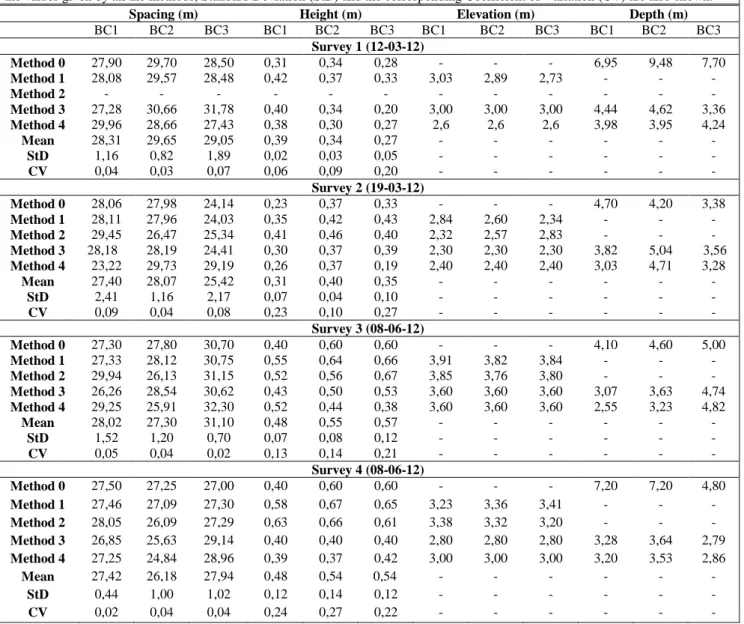
Table 1. Beach cusp (BC) dimensions obtained by each one of the five methods. The mean for each BC obtained from considering the values given by all the methods, Standard Deviation (StD) and the corresponding Coefficient of Variation (CV) are also shown.

Spacing (m) Height (m) Elevation (m) Depth (m)

BC1 BC2 BC3 BC1 BC2 BC3 BC1 BC2 BC3 BC1 BC2 BC3 Survey 1 (12-03-12) Method 0 27,90 29,70 28,50 0,31 0,34 0,28 - - - 6,95 9,48 7,70 Method 1 28,08 29,57 28,48 0,42 0,37 0,33 3,03 2,89 2,73 - - - Method 2 - - - - Method 3 27,28 30,66 31,78 0,40 0,34 0,20 3,00 3,00 3,00 4,44 4,62 3,36 Method 4 29,96 28,66 27,43 0,38 0,30 0,27 2,6 2,6 2,6 3,98 3,95 4,24 Mean 28,31 29,65 29,05 0,39 0,34 0,27 - - - - StD 1,16 0,82 1,89 0,02 0,03 0,05 - - - - CV 0,04 0,03 0,07 0,06 0,09 0,20 - - - - Survey 2 (19-03-12) Method 0 28,06 27,98 24,14 0,23 0,37 0,33 - - - 4,70 4,20 3,38 Method 1 28,11 27,96 24,03 0,35 0,42 0,43 2,84 2,60 2,34 - - - Method 2 29,45 26,47 25,34 0,41 0,46 0,40 2,32 2,57 2,83 - - - Method 3 28,18 28,19 24,41 0,30 0,37 0,39 2,30 2,30 2,30 3,82 5,04 3,56 Method 4 23,22 29,73 29,19 0,26 0,37 0,19 2,40 2,40 2,40 3,03 4,71 3,28 Mean 27,40 28,07 25,42 0,31 0,40 0,35 - - - - StD 2,41 1,16 2,17 0,07 0,04 0,10 - - - - CV 0,09 0,04 0,08 0,23 0,10 0,27 - - - - Survey 3 (08-06-12) Method 0 27,30 27,80 30,70 0,40 0,60 0,60 - - - 4,10 4,60 5,00 Method 1 27,33 28,12 30,75 0,55 0,64 0,66 3,91 3,82 3,84 - - - Method 2 29,94 26,13 31,15 0,52 0,56 0,67 3,85 3,76 3,80 - - - Method 3 26,26 28,54 30,62 0,43 0,50 0,53 3,60 3,60 3,60 3,07 3,63 4,74 Method 4 29,25 25,91 32,30 0,52 0,44 0,38 3,60 3,60 3,60 2,55 3,23 4,82 Mean 28,02 27,30 31,10 0,48 0,55 0,57 - - - - StD 1,52 1,20 0,70 0,07 0,08 0,12 - - - - CV 0,05 0,04 0,02 0,13 0,14 0,21 - - - - Survey 4 (08-06-12) Method 0 27,50 27,25 27,00 0,40 0,60 0,60 - - - 7,20 7,20 4,80 Method 1 27,46 27,09 27,30 0,58 0,67 0,65 3,23 3,36 3,41 - - - Method 2 28,05 26,09 27,29 0,63 0,66 0,61 3,38 3,32 3,20 - - - Method 3 26,85 25,63 29,14 0,40 0,40 0,40 2,80 2,80 2,80 3,28 3,64 2,79 Method 4 27,25 24,84 28,96 0,39 0,37 0,42 3,00 3,00 3,00 3,20 3,53 2,86 Mean 27,42 26,18 27,94 0,48 0,54 0,54 - - - - StD 0,44 1,00 1,02 0,12 0,14 0,12 - - - - CV 0,02 0,04 0,04 0,24 0,27 0,22 - - - -

DGPS based methods to obtain beach cusp dimensions 545

tip” and “lowest point”) allowing the coordinates of the points positioned to be acquired with a high level of accuracy.

In Table 1 results of dimensions measured for each one of the 12 beach cusps (3 from each survey) considered are shown. Also shown are the mean for each beach cusp dimension as well as the standard deviations (StD) and coefficients of variation (CV=StD/Mean). The CV of a variable aims to describe the dispersion of the variable in a way that does not depend on the variable's measurement unit. The higher the CV the greater the dispersion in the variable.

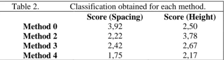
As far as cusp spacing is concerned, all methods seem to produce good results with CV values ranging between 2% and 9%. This means that for a specific beach cusp the spacing value obtained by each method is very similar. CV values regarding cusp height belong to a wider interval than CV values referring to cusp spacing, spanning from 6% to 27%. The CV is useful because it enables comparison of measurements of the different dimensions considered. Thus, from each CV value, it can be said that all methods produce very similar estimates of spacing, while the opposite is true with regard to height. There follows a discussion of the differences in values of spacing and height obtained when comparing values given by method 1 and by all the other methods. A simple classification scheme was devised in order to assess which method provides more similar results to method 1 (in terms of cusp spacing and height). For each cusp measured the difference between the value given by method 1 and the other methods was calculated. For the method in which this difference is the lowest a score of 4 points was given. A score of 1 point was attributed to the method that produced the poorestresult (to the second best method a score of 3 points was given and to the remaining one a 2 point score was attributed). The average was then taken and the results are presented in Table 2. Regarding cusp spacing, method 0 presents the best score. For 11 of the 12 cusps taken into consideration the smallest absolute value of the difference occurs when method 1 is compared with method 0. Method 3 provides slightly better spacing estimates than method 2. For cusp height, method 2 presents the most similar results to method 1.

In order to have an indication of how good a measurement is relative to the size of the thing being measured, we are going to use percent error (Equation 1). Percent error is applied when comparing an experimental quantity, E, with a theoretical quantity, T, which is considered as the correct value of whatever is being measured (here we will consider height and elevation values given by method 1 as those theoretical “correct” values and values given by method 2 as the experimental quantities). The percent error is the absolute value of the difference divided by the “correct” value times 100.

100

*

%

_













 



T

E

T

Error

The maximum and minimum height relative errors take the values of 17.1% and 1.5% respectively. Notice that method 2 only takes into account one measurement to estimate horn tip and “lowest point” elevations so it can easily underestimate or overestimate such elevations. For the calculation of cusp height three points are considered, the elevation of two consecutive “horn tips” and the elevation of the “lowest point” in between them. So in some cases it is possible that these errors cancel each other out (underestimating one of the “horn tip” elevations and overestimating the other, for instance) though the opposite can also occur. Method 4 produces the worst results both in terms of cusp spacing and in terms of cusp height.

In methods 3 and 4 the elevation presented in Table 1 is taken as being equal to the contour value chosen to measure spacing, height and depth. It can easily be seen from Table 1 that method 2 provides better results than method 3 or 4. However, it should be noted that differences between elevation results from method 1 and method 2 can be as high as 0.52 m. The maximum and minimum relative errors (considering method 1 and method 2 in the same way as above) take the values of 20.9% and 1.0% respectively.

Cusp depth is the parameter that is the most difficult to measure because, as has already been pointed out, it is hard to identify the back point in the field, especially if only one person is performing the survey. So, to obtain this dimension, when there is only one person available to perform the field survey we have to rely on the strategy presented in method 3 or 4 and obtain it from the DEM. Differences between depth values obtained via methods 3 and 4 varied, considering all surveys, from a minimum of 0.07m (in the last survey) to a maximum of 0.88 m (in the first survey). Differences between the results obtained via method 3 and 4 probably have, something to do with the problem of choosing different contours to extract the dimensions from, which highlights the importance of choosing an adequate contour and of using objective criteria to select it. For the first survey, method 3 was applied a second time but this time, the contour selected was not the 3.00 m contour, chosen initially, but the 2.6 m contour. In this case results are closer to results obtained by method 4 the maximum difference being equal to 0.36 m. Depth values obtained via method 0 are, in the cases of the first and last surveys, very different from those obtained by the other two methods that provide values for this cusp dimension. The difference can be as high as almost 5 m for BC2 in the 12-03-12 survey.

To finish this section we discuss the sampling and processing times required to perform the survey and to extract cusp dimensions from sampled data. Method 1 requires [(2*n)+1]*30 seconds to sample all “horn tips” and “lowest points” (n being the number of cusps sampled) plus the traveling time in between the first and last “horn tip”. For a set of 3 cusps 5 minutes will be sufficient. For method 2 this time will be in the order of 1-2 minutes. In terms of processing time these two methods have identical required processing times (less than 5 minutes). Method 3 surveying takes longer to finish than all the others and for a 3 cusp system with a mean spacing of 30 meters, 20-25 minutes will be needed to finish the survey. Processing time for this method also takes longer, around 30-45 minutes to process each survey. Method 4 processing time is of the same magnitude as in method 3 and sampling time is less than 1 minute, thus being the fastest one. In method 0 there is no need to process data and it requires around 5-10 minutes of sampling time.

CONCLUSIONS

The purpose of this work is to evaluate different methods to determine beach cusp dimensions, comparing them with each other in order to assess which one produces the most accurate, extensive and easy-to-achieve results.

Method 1 produces more accurate values for all the parameters that it is able to measure, though it is unable to produce results for cusp depth. This dimension is the most problematic to obtain due

Table 2. Classification obtained for each method. Score (Spacing) Score (Height)

Method 0 3,92 2,50

Method 2 2,22 3,78

Method 3 2,42 2,67

546 Lopes, et al.

to the subjectivity inherent in the choice of the contour used to evaluate cusp depth (as seen in methods 3 and 4) and in the difficulty in locating the “backpoint” in the field (in method 0). Methods 3 and 4 produce results for all the 4 dimensions considered. Method 3 results are more accurate than those produced by method 4. The reason for this difference is related to the lower profile density adopted in the latter method.

In terms of spacing, height and elevation results from methods 1 and 2 are easier to obtain, requiring less time to sample and to process the data. In the case of depth, method 0 is the one which involves, once the “backpoint” has been identified, the fewest difficulties to extract the value of this dimension. However, results for depth obtained by method 0 sometimes present, as in the cases of surveys 1 and 4, high dispersion (it should be noted, as the values for all the other dimensions show, that the sets of beach cusps were relatively uniform).

If someone interested in studying beach cusps does not have GPS equipment at his disposal, Method 0 can perfectly be applied for determining cusp spacing.

If one wants to only obtain cusp spacing, elevation and height values, method 1 is recommended owing to its speed in sampling the data and ease in dealing with the data (it requires a little more sampling time than method 2 but it is more reliable).

If one wants cusp elevation, spacing and height but also wants to perform, for instance, analysis of accretional and erosional properties, a DEM will be needed. In this case combining methods 1 and 3 (or methods 1 and 4) surveying techniques is the more appropriate alternative. If one wants to characterize large areas of beach cusps, a combination of methods 1 and 4 is the most appropriate. In relation to processing, spacing, elevation and height can be obtained by method 1 and erosion/accretion maps can easily be produced automatically. There is no need, in this case, to use processing techniques (measurements in AutoCad environment) from method 3 or 4.

If besides the above-mentioned dimensions, one is interested in obtaining cusp depth values, methods 3 or 4 sampling and processing strategies can be used.

Alternatively surveying and processing techniques from methods 1 and 3 (or 4) can be combined together. In this case spacing, height and elevation would be obtained via method 1 sampling and processing strategies. Cusp depth values and erosional / accretional properties would be obtained via method 3 (or 4) sampling and processing strategies. This will enable the shortcoming of method 1, which cannot produce depth results, to be surmounted. At the same time this will permit the use of objective criteria in regard to the value of the topographic contour line to be considered to extract cusp dimensions (in method 3 or 4). The contour line elevation will be equal to the mean elevation of the beach cusp system, which is easily obtained when method 1 is applied.

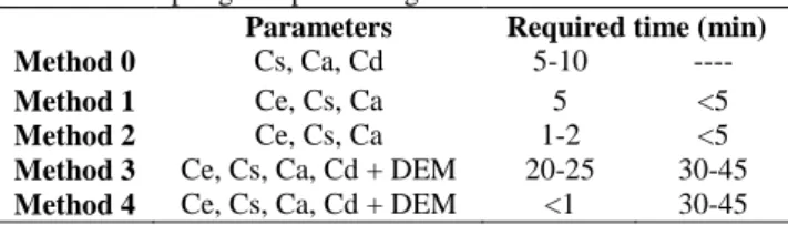
Table 3 shows the parameters that can be measured by each method and the sampling and processing times required to obtain parameter values of a set of 3 beach cusps (with a mean spacing of 30 meters). It also shows which methods can provide DEMs.

As a final remark it is advised to use method 1 when it is intended to measure cusp elevation, height or spacing and to use

method 3 when it is intended to measure cusp depth. In the case that all the four parameters are needed a combination of method 1 and 3 should be used.

ACKNOWLEDGEMENT

This work is financed by Fundação para a Ciência e Tecnologia (FCT), grant reference SFRH/BD/45292/2008. Paulo Baptista was supported by the FCT, grant reference SFRH/BPD/63141/2009. The authors would like to thank FCT, Portugal, for the financial support of Project MoZCo (PTDC/ECM/099999/2008).

LITERATURE CITED

Almar, R., Coco, G., Bryan, K. R., Huntley, D. A., Short, A. D. and Senechal, N., 2008. Video observations of beach cusp morphodynamics.

Marine Geology. 254, 216-223.

Aoki, T. and Sunamura, H., A., 2000. Laboratory Experiment on the Formation and Morphology of Beach Cusps. Transactions of Japanese

Geomorphological Union, 21, 291-306.

Baptista P., Cunha T., Matias A., Gama C., Bernardes C. and Ferreira Ó., 2011a. New land-based method for surveying sandy shores and extracting DEMs: the INSHORE system. Environmental Monitoring

and Assessment, 182, 243-257.

Baptista P., Cunha T.R., Bernardes C., Gama C., Ferreira Ó. and Dias A., 2011b. A precise and efficient methodology to analyse the shoreline displacement rate. Journal of Coastal Research, 27, 223-232.

Benavente, J., Harris, D.L., Austin, T.P. and Vila-Concejo, A., 2011. Medium term behavior and evolution of a beach cusps system in a low energy beach, Port Stephens, NSW, Australia. In: Furmanczyk ,K.,Giza, A. and Terefenko, P. (eds.), Proceedings of the 11th _{International}

Coastal Symposium (Szczecin, Poland), Journal of Coastal Research,

Special Issue No.64, pp. 170-174.

Coco, G., O'Hare, T.J. and Huntley, D.A., 1999. Beach cusps: a comparison of data and theories for their formation. Journal of Coastal

Research, 15, 741–749.

Coco, G., Burnet, T. K., Werner, B. T. and Elgar, S., 2004. The role of tides in beach cusp development. Journal of Geophysical Research C:

Oceans, 109:4.

Cunha, T., 2002. High Precision Navigation Integrating Satellite

Information - GPS – And Inertial System Data. Porto, Portugal:

University of Porto, PhD thesis, 215p.

Holland, K. T. and Holman, R. A., 1996. Field observations of beach cusps and swash motions. Marine Geology, 134, 77-93.

Holland, K. T., 1998. Beach cusp formation and spacings at Duck, USA.

Continental Shelf Research, 18:10, 1081-1098.

Lopes, V, Pais-Barbosa, J, Taveira-Pinto, F and Veloso-Gomes, F., 2011. Beach cusps: Using multivariate data analysis techniques for the identification of important variables and for predicting their spacing. In: Furmanczyk ,K.,Giza, A. and Terefenko, P. (eds.), Proceedings of the

11th International Coastal Symposium (Szczecin, Poland), Journal of Coastal Research, Special Issue No 64, pp. 1106-1110.

Masselink, G., 1999. Alongshore variation in beach cusp morphology in a coastal embayment. Earth Surface Processes and Landforms. 24, 335-347.

Nolan, T. J., Kirk, R. M. and Shulmeister, J., 1999. Beach cusp morphology on sand and mixed sand and gravel beaches, South Island, New Zealand. Marine Geology, 157, 185-198.

Pais-Barbosa, J., 2007. Hidromorfologias e Hidroformas Costeiras Locais (in Portuguese). Porto, Portugal: University of Porto, PhD thesis, 780p. Rasch, M., Nielsen, J. and Nielsen, N., 1993. Variations of spacings

between beach cusps discussed in relation to edge wave theory.

Geografisk Tidsskrift, 93, 49-55.

Takeda, I. and Sunamura, T., 1983. Formation and Spacing of Beach Cusps. Coastal Engineering in Japan. 26, 121-135.

Vousdoukas, M.I., 2012. Erosion/accretion patterns and multiple beach cusp systems on a meso-tidal, steeply-sloping beach

Geomorphology, 141-142, 34-46.

van Gaalen, J.F., Kruse, S.E., Coco, G., Collins, L. and Doering, T., 2011. Observations of beach cusp evolution at Melbourne Beach, Florida, USA. Geomorphology 129, 131–140.

Table 3. Sampling and processing times for each method Parameters Required time (min)

Method 0 Cs, Ca, Cd 5-10 ----

Method 1 Ce, Cs, Ca 5 <5

Method 2 Ce, Cs, Ca 1-2 <5

Method 3 Ce, Cs, Ca, Cd + DEM 20-25 30-45 Method 4 Ce, Cs, Ca, Cd + DEM <1 30-45