Electromagnetic and Thermal Aspects of a FFC-NMR Equipment Magnet and Power Supply

Electromagnetic and Thermal Aspects of a Fast Field

Cycling NMR Equipment

Magnet and Power Supply

Bruno Pereira

Depart. Elect. and Comp. Engineering Insituto Superior Técnico Universidade de Lisboa, Portugal bruno.i.pereira@tecnico.ulisboa.pt

Duarte M. Sousa

Depart. Elect. and Comp. Engineering Instituto Superior Técnico and INESC-ID

Universidade de Lisboa, Portugal duarte.sousa@tecnico.ulisboa.pt

António Roque

Department of Electrical Engineering

ESTSetúbal - Instituto Politécnico de Setúbal & INESC-ID Setúbal, Portugal

antonio.roque@estsetubal.ips.pt Abstract— The Fast Field Cycling Nuclear Magnetic

Resonance (FFC-NMR) technique has been spreading its application to new areas such as oil and food industry. Consequently, new features and improvements concerning the equipment available has been investigated and exploited. Under this context, this paper describes the main aspects concerning the electromagnetic and thermal behavior of the main power supply and the magnet, respectively. The proposed power supply and the magnet were developed under the specifications of the FFC-NMR equipment and in order to match the requirements of the most recent areas of application. The dynamic behavior of the power supply is analyzed based on simulation results, being the thermal study of the magnet performed using finite element method software.

Keywords— Spectrometer; Power Supply; Magnet; Nuclear Magnetic Resonance; Fast Field Cycling; Thermal Study

I. INTRODUCTION

The Fast Field Cycling Nuclear Magnetic Resonance (FFC-NMR) is an experimental technique used to study the the molecular dynamics of different types of compounds. This technique has a high use in various research areas such as Physics, Chemistry, Medicine, and Pharmacy, among others. This technique requires relaxometers that allow switching the magnetic flux density quickly, accurately and in a repetitive way. As first approach, the switching times are within the millisecond range and maximum magnetic flux density is 0.2T [1-3].

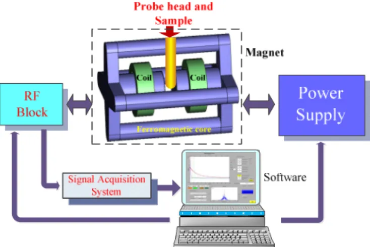
In Fig. 1, the main blocks of a NMR spectrometer are represented. Among other circuits and components, a FFC-NMR needs a specific magnet and a fast suitable power supply. The power supply is a current source, which must allow rapid transitions of the current, i.e., switching the current between 0 and 10 A within the time range 3 to 6 ms (ton and toff, see Fig.

2). Furthermore, the current ripple should be as low as possible

in order to guarantee an accurate magnetic flux density (B0)

and a very high homogeneity given by the expression (1) [4].

∆

=

The Fast Field Cycling technique is used to determine the longitudinal relaxation time (T1) over a range of the magnetic

flux density not covered by classical NMR techniques. In this work, the proposed solution covers a flux density range from 0 T to 0.4 T, corresponding to a magnet current range from 0 to 10A, as referred before. Doubling the maximum magnetic flux density, the proposed power supply and magnet will contribute to expand the range and type of samples that can be studied with this technique.

Fig. 1. Main blocks of a FFC NMR spectrometer

FFC magnets are designed according a target flux density B0. In general the homogeneity of the magnetic flux density is

considered the most important requirement for the magnet [1-2,5], however, it should also have minimum power losses.

FFC-NMR spectrometers have been evolved taking advantage of the evolution of power electronics devices and magnet design techniques.

In this paper, a different solution for the power supply of the FFC-NMR spectrometer is described and simulated. The main results concerning the temperature distribution in the magnet are also shown.

II. THE POWER SUPPLY

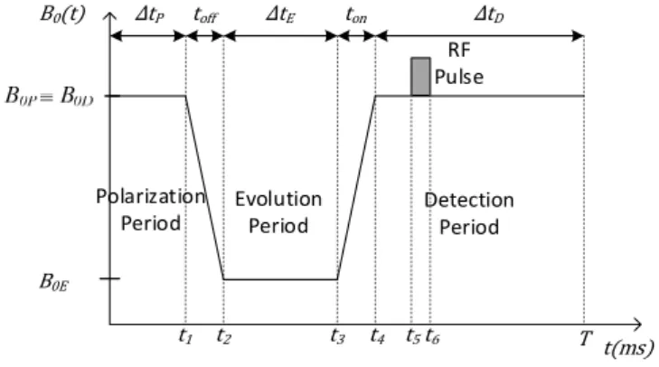
During a normalized FFC-NMR experiment the magnetic flux density cycles as represented in Fig. 2. During a cycle, the following stages are observed:

1. The sample is polarized with a high magnetic flux density B0P (polarization field) during a time interval

ΔtP, until the nuclear magnetization of the sample

achieves saturation, i.e., [6]

∆ 5 ( ) (2)

2. The magnetic flux density is switched to a value B0E

(evolution field), lasting at this level for a time ΔtE

during which the nuclear magnetization relaxes towards a new equilibrium value.

3. The magnetic flux density is switched to a value B0D

(detection field) and the sample is excited by the RF pulse. The sample’ response is detected and acquired by the RF unit tuned to a predetermined frequency respecting the Larmor frequency of the molecular element under study. After cessing the RF pulse is detected the signal (FID - Free Induction Decay), that is used to determine T1.

The polarization field (B0P) and detection field (B0D) may

have different values, being usually B0P ≥ B0D [1-2,6].

B0P=B0D B0E B0(t) t(ms) ΔtD ton ΔtE ΔtP toff Evolution Period Detection Period Polarization Period RF Pulse t1 t2 t3 t4 t5t6 T

Fig. 2. Normalized field cycle

The project of a power supply for a FFC-NMR magnet includes several requirements and can be based on different assumptions. The magnet current should behave as a current source allowing fast current switching times in order to obtain

a magnet flux density cycling as represented in Fig. 2 [7-8]. In this work, it is also assumed that the characteristic magnetic flux density vs. magnet current is linear and that the power supply should contribute to get fast magnet current transients.

The power supply should be able to control the magnet current from 0 to 10A and the response times of the current transitions within the range 3 to 6 ms.

The design of the magnet influences the project of the power supply, mainly their electric resistance, Rm and

self-inductance Lm. In this paper was considered a magnet

developed recently [9] with self-inductance of 0.2 H and electrical resistance of 3Ω.

When setting up the power supply topology, it should be considered fully controllable semiconductor, i.e., it should be considered the possibility of controlling the operating point of the semiconductors in addition to the typical "ON" and "OFF" states.

A. Electric circuit

The circuit shown in Fig. 3 represents the proposed power supply. This circuit is constituted by two voltage sources (V and Vaux), diodes (D, Daux and DRL), switches (IGBTs S and

Saux) and a RC filter (C and RC), being the load the magnet with

parameters Rm and Lm. To analyze the dynamic behavior and

the operating principles of this circuit, 3 operating modes are considered:

• steady state; • “up” transient; and • “down” transient.

Fig. 3. Electric circuit of the power supply

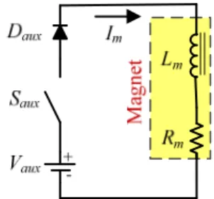
1) Steady State:

In steady state (current regulated), Vaux remains

disconnected (Saux is “OFF”), being the equivalent circuit

represent by Fig. 4.

Fig. 4. Electric circuit in steady state

If the semiconductor S is "ON", the current flows from the voltage source V to the magnet, being the diode DRL “OFF”.

During this process, the capacitor C discharges through the resistor RC. Neglecting the voltage drop of the semiconductors

(switch and diode), in steady state the magnet current is regulated knowing that:

= 1 (3)

If S is “OFF”, the energy stored in the coil will be transferred to the capacitor. During this transition the energy is dissipated in the resistance Rm. However, the amount of energy

transferred from the inductor to the capacitor is very small, since the purpose is to keep the current constant.

2) “Up” transient:

In Fig. 5, it is shown the equivalent circuit during the “up” transient.

Fig. 5. Electric circuit for the “up”transient

During the “up” transient the semiconductor Saux is “ON” (S

is “OFF” avoiding short-circuiting the voltage sources). The control systems is designed to detect when the magnet current reaches the target current level, switching Saux “OFF” and

changing the operation mode to “steady state”. The time evolution of the magnet current is:

= 1 (4)

Since Vaux>>V, the magnet current dynamics is accelerated

in order to fulfill the requirements of the application. 3) “Down” transient:

During the “down” transient the magnet current path is represented in Fig. 6.

Fig. 6. Electric circuit for the “down”transient

According to Fig. 6, during the “down” transient the energy stored in the magnet is transferred to the capacitor C. Since the impedance of the resistance is much higher than the impedance

of the capacitor (ZRc>>ZC), the current flows through the diode

DRL being neglected the current flowing through the resistor RC.

In this situation it is intended that the current drops very fast, so the amount of energy transferred from the inductor to the capacitor is large. The energy transfer rate is responsible for decreasing the magnet current as fast as possible.

When the current reaches the reference value, the semiconductor S is set to “ON” and the system goes into steady state, again.

III. CONTROL SYSTEM

In Fig. 7, the circuit with a closed loop control chain is shown. A core point is the design of the magnet current regulator. In Fig. 8 the block diagram of the proposed solution in order to set the regulator parameters is represented.

Fig. 7. Diagram of the circuit with the regulation chain

T s K a + 1 R ⎜⎜_⎝⎛ +s_RL ⎟⎟_⎠⎞ m m m1 1

Fig. 8. Block diagram of the regulation chain

In Fig. 8, the block C(S) represents the regulator, the central block represents the dynamic model of the switched converter, being Ta a time constant related with the statistical

delay caused by characteristic delays in the command system and K is the gain of the converter. The third block represents the transfer function of the magnet.

A PI (proportional and integral action) controller is used to control the circuit, ensuring a fast response and a null static error. Being the typical transfer function of the PI controller:

( ) = ( )

( ) ( )=

=

=

To determine the regulator parameters (KP and KI) the

modulus optimum technique is used [10]. This technique cancels the dominant pole of the load with a zero of the regulator, i.e., the time constant TZ is given by:

=

system can be represented by:

( )

( )

=

=

For this type of system, the static speed error should be minimized. Using the ITAE criteria, the 2rd order optimized transfer function is given by [10-11]:

( ) =

√ (8)

Considering (7) and (8), the following expressions, under optimized conditions, are obtained:

=

√2

=

Solving the previous equation system:

=

The proportional and integral gains, can be estimated using:

=

=

The current error is given by:

( ) = ( ) =

=

( )

( ) (13)

By the final value theorem, taking into account that the reference is a step (

( )

lim ( ) ( ) = = 0 (14)

IV. SIMULATION RESULTS

The proposed solutions for the power supply together with the control system are analyzed by simulation. In Fig. 9 the simulation model is represented. The block "Selector" is responsible for selecting the operation mode avoiding

short-circuits between the voltage source V and the auxiliary voltage source Vaux (a dead time is considered between the sequences

“OFF” – “ON” of the switches).

To compute the simulations a regulator with the following gains is considered:

• KP=1;

• KI=15;

• KW=1.

Fig. 9. Simulation model of the power supply

The simulation results are obtained having as reference the normalized field cycle (Fig. 2). The reference current waveform is set with parameters that are typical of a real FFC experiment. The current levels ID and IE are proportional to the

flux density levels B0D and B0E, respectively.

The parameters used are: • ID = 10 A;

• IE = 4 A;

• ton = 3 ms;

• toff = 6 ms.

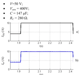
In Fig. 10 the simulation result of the magnet current is shown. In Fig. 11 and Fig. 12 the “up” and “down” transients are illustrated, respectively. To perform the simulations the values of other parameters are:

• V=50 V; • Vaux = 400V;

• C = 147 µF; • RC = 280 Ω.

Fig. 10. Simulation result of the magnet current: a) reference current; b) magnet current

The C value was designed considering the power stored in the magnet (WL) and the voltage variation (ΔvC) that is

observed when during a current “down” transient, i.e.,

=

∆ . For other hand, RC>>(1/ωC) in order to obtain the

required system dynamics.

a)

b)

Fig. 11. Simulation result of the magnet current during the “up” transient”: a) reference current; b) magnet current

IRef (A ) Im (A ) a) b)

Fig. 12. Simulation result of the magnet current during the “down” transient”: a) reference current; b) magnet current

IRef (A) Im (A ) a) b) 2A 4A 10A 2A 4A 10A

Fig. 13. Simulation result of the magnet current for an enlarged cycle: a) reference current; b) magnet current

Fig. 14. Simulation result of the magnet current ripple for different current levels: a) 4A; b) 2A; c) 10A

In Fig. 13 it is shown the simulation result for an enlarged current cycle. In Fig. 14, the current ripple corresponding to the different current levels set to the enlarged cycle is shown.

The simulation results allow verifying that the current dynamics fulfills the requirements of the application. For other hand, the current ripple for the maximum current (10A) can be seen as a drawback of the proposed solution. Anyway, the ripple could be reduced increasing the switching frequency of the semiconductors.

V. THERMAL STUDY OF THE MAGNET

The magnet designed to be used with the proposed power supply is shown in Fig. 15. This magnet is based on a ferromagnetic core with two set of coils placed in the central leg, which has an air-gap where the sample submitted to a FFC NMR experiment is placed.

Fig. 15. 3D representation o the magnet [9]

The performance of the FFC NMR equipment depends on the thermal behavior of their components. All elements that constitute the magnet are affected and responsible by the heat transfer processes that occur inside of it. So that, it becomes important to evaluate the magnet temperature distribution and define the cooling requirements of the magnet, at least to assure that the materials temperature specifications are not violated.

To evaluate the magnet temperature distribution, a study is performed using a 2D finite element software (FEMM). An example of the output obtained with these simulations is shown in Fig. 16.

Fig. 16. Temperature distribution in the magnet

According to the temperature distribution observed, there is a standard behavior that allows getting the average temperature for the three main parts of the magnet: ferromagnetic core, windings and air gap. In Table I the average temperature for these three points for different values of the power losses is shown, which are the main heat source of this system.

The results summarized in Table I, point out clearly that the magnet requires forced ventilation. In Table II are summarized the temperatures, for the same points, with ventilation. The real magnet is encapsulated including a fan that cools the magnet extracting the air contacting the hot parts of this system.

TABLE I. TEMPERATURES INSIDE THE MAGNET WITHOUT FORCED VENTILATION ( ) ( ) ( ) ( ) 100 53.85 46.35 46.65 200 83.65 68.65 69.25 300 113.55 91.05 91.85 400 143.35 113.35 114.45 500 173.15 135.65 137.15

TABLE II. TEMPERATURES INSIDE THE MAGNET WITH FORCED VENTILATION ( ) ( ) ( ) ( ) 100 30.95 30.15 30.25 200 37.85 36.25 36.45 300 44.75 42.35 42.75 400 51.65 48.45 48.95 500 58.55 54.55 55.15 VI. CONCLUSION

The electric circuit and control system analyzed in this paper allow obtaining results that are under the specifications of the FFC-NMR technique. The proposed solution constitutes a great improvement since its target magnetic flux density is much higher than other solutions with similar features.

The analyzed system allows obtaining a magnetic flux density up to 0.4 T (corresponding to a magnet current of 10A). This magnetic flux density level allows setting the FFC equipment, not only with the proton specifications, but also considering fluorine atoms.

The designed magnet matches with the proposed solution for the power supply. This magnet is portable (important advantage than other FFC magnets) and can be cooled by a simple fan.

ACKNOWLEDGMENT

This work was supported by national funds through FCT – Fundação para a Ciência e a Tecnologia, under project UID/CEC/50021/2013.

REFERENCES

[1] 4Décorps, M.: "Imagerie de Résonance Magnétique", EDP Sciences et CNRS Éditions, ISBN EDP Sciences 978 2 7598 000 1 et CNRS Éditions 978 2 271 07233 7, pp.31, 1987.

[2] 3 F. Noack, “NMR Field-Cycling Spectroscopy: Principles and Applications”, Prog. NMR Spectrosc., vol. 18, pp. 171-276, 1986. [3] 6 R. Seitter, R. O. Kimmich, “Magnetic Resonance: Relaxometers”,

Encyclopedia of Spectroscopy and Spectrometry, Academic Press, London, pp. 2000-2008, 1999.

[4] 2 E. Anoardo, G. Galli, G. Ferrante, “Fast-Field-Cycling NMR: Applications and Instrumentation”, Applied Magnetic Resonance, vol. 20, pp. 365-404, 2001.

[5] 1 R. Kimmich and E. Anoardo, “Field-Cycling NMR relaxometry”, Progress in NMR Spectroscopy, 44, pp. 257-320, 2004.

[6] 5 J. Constantin, J. Zajicek, F. Brown, “Fast Field-Cycling Nuclear Magnetic Resonance Spectrometer”, Rev. Sci. Instrum., vol. 67, pp. 2113-2122, 1996.

[7] A. Roque, S. F. Pinto, J. Santana, Duarte M. Sousa, E. Margato, J. Maia, “Dynamic Behavior of Two Power Supplies for FFC NMR Relaxometers”, IEEE International Conference on Industrial Technology – ICIT 2012, Athens - Greece, 2012.

[8] D. M. Sousa, G. D. Marques, J. M. Cascais, P. J. Sebastião, “Desktop Fast-Field Cycling Nuclear Magnetic Resonance Relaxometer”, Solid State Nuclear Magnetic Resonance, vol. 38, pp. 36-43, 2010.

[9] A. Roque: “Flux density distribution of a magnet with axial symmetry to be used in FFC-NMR”, International Conference on Superconductivity and Magnetism 60 (ICSM), Turquia 2014.

[10] A. Roque, G.D. Marques, D. M. Sousa, E. Margato, J Maia: “Control of a Power Supply with Cycling Current Using Different Controllers”, International Symposium on Power Electronics, Electrical Drives, Automation and Motion (SPEEDAM), 2014.

[11] K. Ogata, “Modern Control Engineering”, 5th Edition, Prentice-Hall 2010.