Abstract— The transverse flux permanent magnet machines have
become an interesting possibility for offshore wind turbines. These machines have the highest relation between electrical torque and weight of active materials. The pole pair modular construction could eliminate or lower the gear ratio used in conventional wind turbines. This paper presents a dynamic model of a wind turbine equipped with a transverse flux permanent magnet generator connected to a direct-current power system using a combination of 3D finite element generator model and an aerodynamic model. The results indicate that the model can give accurate response for steady-state operation and for wind speed variations.
Index Terms— electrical machines, finite element analysis, permanent magnet, transverse flux generator, wind turbines.
I. INTRODUCTION
Offshore wind power is a very prominent research theme. Most of the European countries with high
amount of wind power (like Germany, United Kingdom, Ireland, Denmark, Netherlands, Sweden) are
planning to build a huge number of offshore wind farms in the next years [1]-[2]. Some of them will
be installed up to 100 km from the land with 1 GW of capacity. The Europe’s installed offshore wind
power is expect to reach 40 GW by 2020. By the end of 2009, the total installed offshore wind power
in Europe has reached more than 2 GW in 830 grid connected wind turbines [1]. These wind turbines
are grouped in 39 wind farms in nine countries. The largest wind farm is placed in Denmark (209
MW, Horns Rev 2). The most effective transmission system to connect the wind farms to the shore is
not already defined, however, there is a tendency to use a direct-current offshore grid in order to
collect the generated power produced by a group of wind farms in a common offshore substation [2].
The initial cost of an offshore wind farm can be twice as much as the equivalent onshore [3].
In the last 10 years, the use of permanent magnet materials has been increasing considerably. This
fact has contributed to the development of new concepts of electrical machines for new application
[4]. Comparative studies about wind generators have shown that permanent magnet generators (PMG)
has many advantages when compared to the conventional doubly-fed induction generator (DFIG) or
even with the synchronous generator with electrical excitation [5]. As a general rule, PMG can be
Dynamic Modeling of Transverse Flux
Permanent Magnet Generator
for Wind Turbines
Maurício B. C. Salles, José R. Cardoso,
LMAG - Laboratory of Applied Electromagnetism University of São Paulo – Brazil e-mail: [email protected]; [email protected]
Kay Hameyer
divided according to the direction of the magnetic flux in relation to their shafts as: radial
(conventional), axial and transversal. Since the transverse flux permanent magnetic machine (TFPM)
has the highest relation between electrical torque and mass (their size is even smaller than
conventional PMG for the same nominal torque), this concept deserves special attention [4]-[7].
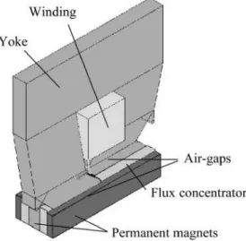
The dynamic behavior of most electrical machines can be studied by the use of analytical equation,
however, it is not the case of the TFPM (shown in Fig. 1). The constructive geometry of the TFG is
very complex and has no 2D symmetry. The intuitive solution to model its dynamic is the approach
which connects the dynamic model of the electrical power system and the controllers step-by-step to
the TFG 3D finite element model. On the other hand, the required simulation time to process this
analysis is impractical. For this reason, a hybrid model was developed allowing fast dynamic analysis
of wind turbines equipped with TFG.
Fig. 1 The 3D view of the TFPM built at IEM - RWTH Aachen University.
This paper is organized as follows. Section II presents a brief description of the TFG. The 3D finite
element analysis (FEA) of this generator is described in Section III. The wind turbine dynamic model
is presented in Section IV. The dynamic analysis of the TFG is presented in Section V. In Section VI,
the main conclusions are summarized.
II. TRANSVERSE FLUX PERMANENT MAGNET MACHINE
The transversal flux permanent magnet machine was first developed to operate as a motor in the
80’s by H. Weh [4],[6],[7]. More than 11 geometries of transverse flux permanent magnet machines
(TFPM) have been described in the literature [8]. Among them is also highlighted that
flux-concentrating TFPM provide higher force density compared to surface-mounted TFPM [8]. More
research has been done in the motor operation, however, the operation as generator is very similar.
At the Institute of Electrical Machines (IEM), RWTH Aachen University, a three-phase
configuration of TFPM with flux-concentrating was developed. This machine was previously
shown in Fig. 2. The operation of TFPM is very similar to the conventional synchronous machine
allowing similar control strategies [7]. The nominal characteristics of the TFPM prototype developed
in Aachen are: 25 kW; 600 rpm; 400 Nm; 205 V; 70 A.
The eddy currents losses calculated using three dimensional finite element analysis of the Aachen
TFPM prototype was presented in [9]. The complex construction of the TFPM requires expensive soft
magnetic composites and is justified for special and critical applications [10].
III. DYNAMIC ANALYSIS METHOD FOR TRANSVERSE FLUX PERMANENT MAGNET MACHINE
The dynamic analysis of conventional electrical machines is performed using dynamic analytical
equation for each phase winding. In the case of the TFPM, the most appropriate form to analyze its
dynamic behavior is with the use of the finite element modeling. Duo to the complex constructive
geometry, there is no symmetry considering two-dimensional axis (2D symmetry). By consequence,
the analysis must be in the three-dimensional axis, some simplifications may be done.
Due to its construction, the phase windings are exactly the same and the flux linkage between each
other can be neglected. This fact allows the analysis of only one phase to determine the flux linkage
(λ) and the electromagnetic torque (Te). The modular configuration of the TFPM enables the finite
element method to be performed in only one pole pitch (Fig. 2). The saturation effect is taking into
account considering the non-linear characteristic of the core material. The flux linkage in phase A can
be determined by the finite element method applied to the mesh geometry shown in Fig. 3. In
addition, the general electrical machine theory can be used to determine the induced voltage in each
winding using the equation (1).
Fig. 2 Linearized pole pitch of the phase A (permanent magnets in rotor).
A. Determination of the Flux Linkage (λ)
The terminal voltage of the TFG can be determined differentiating the flux linkage of the stator windings, as shown in equation (1).
(
,
)
( )
( )
d
i
v t
R i t
dt
λ
θ
= − ⋅
+
(1)This equation is a general form of stator voltage for alternating current generators [7]. The flux
linkage is computed as function of rotor position and armature currents by 3D static finite element
analysis [7]. The form of equation (1) must be expanded to implement the look-up table data:
(
,
)
(
,
)
( )
( )
d
i
di
d
i
d
v t
R i t
di
dt
d
dt
λ
θ
λ
θ
θ
θ
= − ⋅
+
⋅
+
⋅
(2)Finally, the current differential term of the equation is isolated and implemented in
Matlab/Simulink:
(
)
(
)
,
( )
( )
,
md
i
di
di
v t
R i t
dt
d
d
i
λ
θ
ω
θ
λ
θ
=
+ ⋅
−
⋅
⋅
(3)where v(t) is the terminal voltage; R is the phase resistance; i(t) is the phase current; t is time; θ is the
rotor angular position of the electric system; ωm is the rotor velocity.
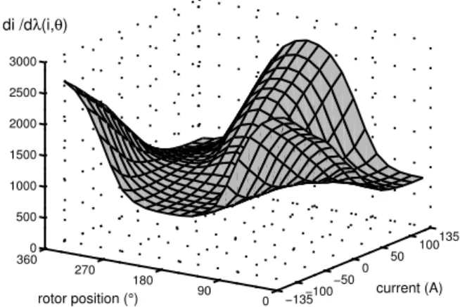
With the flux linkage determined by the 3D static FEA, the two differential terms of the right side
of the equation (3) can be calculated. The first term of equation (3), the values of flux linkage
obtained from the static analysis are derived in relation to the current, for example, the rotor position
is fixed in 10º and two values of flux linkage related to consecutive current are derived. For the
second term, the values are derived in relation to the rotor position, for example, current is fixed in 1
A and two values of flux linkage related to consecutive rotor positions are derived. These values are
interpolated and showed in Fig. 4 and Fig. 5, respectively. Using this approach one can simulate the
transient and the static behavior of the TFG by combining the analytical equations and the look-up
tables. This approach facilitates the implementation of the equation (3) via two look-up tables.
−135−100 −50 0 50 100 135 0 90 180 270 360 −0.08 −0.06 −0.04 −0.02 0 0 0.02 0.04 0.06 0.08 current (A) rotor position (°)
dλ(i,θ) /dθ
Fig. 4 Interpolation of the first differential term.
−135−100 −50 0 50 100 135 0 90 180 270 360 0 500 1000 1500 2000 2500 3000
rotor position (°) current (A)
di /dλ(i,θ)
B. Determination of the Electromagnetic Torque (Te)
During the computation of the flux linkage of the TFG phase A, the values of the respective
electromagnetic torque were also calculated as function of rotor position and armature currents using
the equation (4) [7]:
(
,
)
( )
A A AA
e A
A
d
i
T
i t
p
d
λ
θ
θ
=
⋅
⋅
(4)where p is the number of pole pairs.
The interpolation of these values is shown in Fig. 6. They are also implemented as a look-up table
in the Matlab/Simulink model. The rotor position of the values related to phase B and phase C is
dislocated by – 120º and +120º respectively. The magnetic decoupling between phases makes possible
the individual phase simulation. Equation (5) shows the total electromagnetic torque (TE) produced by
the superposition of the stator phases (A, B and C) of the TFG.
A B C
E e e e
T =T +T +T (5)
−135−100 −50 0
50 100 135
0 90 180 270 360 −450 −300 −150 0 150 300 450
current (A)
rotor position (°)
Te (Nm)
Fig. 6 Electromagnetic torque of the phase A.
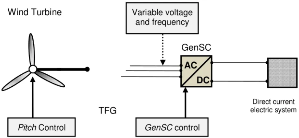
IV. WIND TURBINE MODELING
The TFG requires a full converter in order to operate in variable speed. This fact enables the wind
turbine to maximize the generated power.
Direct current electric system
AC
DC
GenSC
TFG Wind Turbine
GenSC control Pitch Control
Variable voltage and frequency
The aerodynamic model, the generator model and the converter control model are described in the
following topics.
A. Aerodynamic Model
For all kinds of wind turbine technologies the energy conversion principle is the same. The
mechanical power (Pm) capture from the wind by a wind turbine and its related mechanical torque
(Tm) can be calculated using the well-known aerodynamic equations [2]-[5],[11]:
(
)
3
1
,
2
m wt P wt
P
= ⋅ ⋅ ⋅
A
ρ
V
⋅
C
λ
β
(6)m m
wt
P
T
ω
=
(7)where A is the turbine rotor area, ρ is the air density, Vwt is the wind speed, Cp is the performance
coefficient, β is the blade pitch angle, λwt = ωwtRwt /Vwtis the tip speed ratio, Rwt is the radius of the
turbine rotor and ωwt is turbine angular speed.
The performance coefficient depends on the blade pitch angle and the tip speed ratio (λwt). Usually,
a group of curves are experimentally obtained by the manufacture of the wind turbine. However, for
these studies we have used the analytical equation proposed in [2],[11]. The pitch angle control
diminishes mechanically the Cp of the wind turbine in order to limit the generated power for wind
speeds higher than the nominal. The adopted pitch angle control operates as electric power regulator
[11] and is activated only when the velocity of the wind turbine reaches its nominal value (21,8 rpm).
The adopted 2 MW wind turbine [11] requires a gear box (GB) ratio 1:27,5 to match the nominal
generator speed.
B. Generator Model
The analytical dynamic equations of generators are sufficient for most of the studies. Therefore,
there are no well-know dynamic equations for TFG and the approach using look-up tables is required,
as described in section III. Additionally, the mechanical equations were implemented:
(
)
1
mm E
d
T
T
dt
J
ω
=
⋅
−
(8)m d
dt
θ
=ω
(9)
where TEis the sum of the electromagnetic torque of the 3 phases, J is the combined inertia coefficient
(sum of the turbine rotor and the generator rotor) and θ is the mechanical rotor angular position.
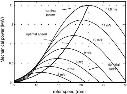
The nominal mechanical characteristics of the adopted wind turbine do not match to the nominal
characteristics of the TFPM prototype, hence the concept of per unit systems (p.u. systems) must be
used as suggested in [2]. The operation of the generator must follow the best rotor speed in order to
maximize the mechanical power. In Fig. 8, the optimized power tracking is obtained by adjusting the
turbine-generator angular speed for each wind velocity.
C. Converter Control Model
considering also the performance coefficient and the blade pitch control (Fig. 8). The more
appropriate offshore transmission system to bring the electrical power to the land is not already
defined, however, there is a tendency to use the HVDC transmission system in some far locations. For
this reason, the converter model used in this study represents only an ideal IGBT-based machine side
converter connected to an internal direct-current (dc) network of the wind farm.
5 10 15 20 25 30
0 0.5 1 1.5 2
rotor speed (rpm)
Mechanical power (MW)
11.8 m/s
6 m/s 7 m/s
8 m/s
10 m/s
9 m/s
11 m/s
optimal speed nominal
power
nominal speed
Fig. 8 Output power for different values of wind speed (m/s).
The PWM (Pulse-width modulation) converter control (show in Fig. 9) employs dq0 rotating
reference frame to vary the applied voltage and frequency to active optimal speed.
encoder
PI +
_
ω
r*opt(rpm)
ωr(rpm)
I*q
dq0
abc
θ
I*d = 0
I*abcs
Current controller
Iabcs
V* abcs
Fig. 9 Block diagram of the converter control.
The terms with the mark (*) are the reference values. In this figure, Iabc are the phase currents
injected by the generator into the dc network. The symbol θ is the rotor position reference to the dq0
-to-abc transformation. The speed controller is implemented with a proportional and integral regulator
(PI), it is responsible for providing the quadrature current reference (Iq *
). The direct-axis reference
current (Id *
) is 0 (zero) in order to maximize the electromagnetic torque (TE) [12],[13]. After a dq0
-to-abc transformation, the three-phase reference currents are compared at the current controller which
gives the converter output reference voltages (V*abc). The reference voltages are sent to the PWM
V. DYNAMIC ANALYSIS OF WIND TURBINE
Two different dynamic studies were performed in order to check the behavior of the model
presented in sections III and IV. The first one analyzes the steady-state characteristics and the second
one analyzes the dynamic behavior of the wind turbine based on TFG during wind gust perturbation.
A. Steady-State Characteristic with Constant Wind
One dynamic simulation was performed for each wind speed value in the range from 0,5 m/s to 20
m/s. The values of the steady-state operation point for optimal mechanical power (shown in Fig. 8)
are compared to the electric power effectively injected into the DC grid. As the only considered losses
are the cooper losses, one can see in Fig. 10 the agreement of both values.
0 2 4 6 8 10 12 14 16 18 20
0 0.5 1 1.5 2
wind speed (m/s)
o
u
tp
u
t
p
o
w
e
r
(M
W
) mechanical
electric
Fig. 10 Estimation of the wind turbine power curve.
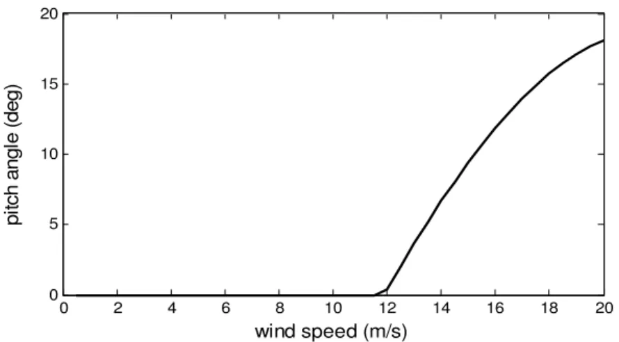
The blade pitch angle position is shown in Fig. 11, one can see the different steady-state values
assumed by the control to diminishes the power captured when the wind speed is over the nominal
speed (11,8 m/s) to guarantee that the generator is not overloaded.
0 2 4 6 8 10 12 14 16 18 20
0 5 10 15 20
wind speed (m/s)
p
it
c
h
a
n
g
le
(
d
e
g
)
Fig. 11 Position of the blade pitch angle for different wind speed.
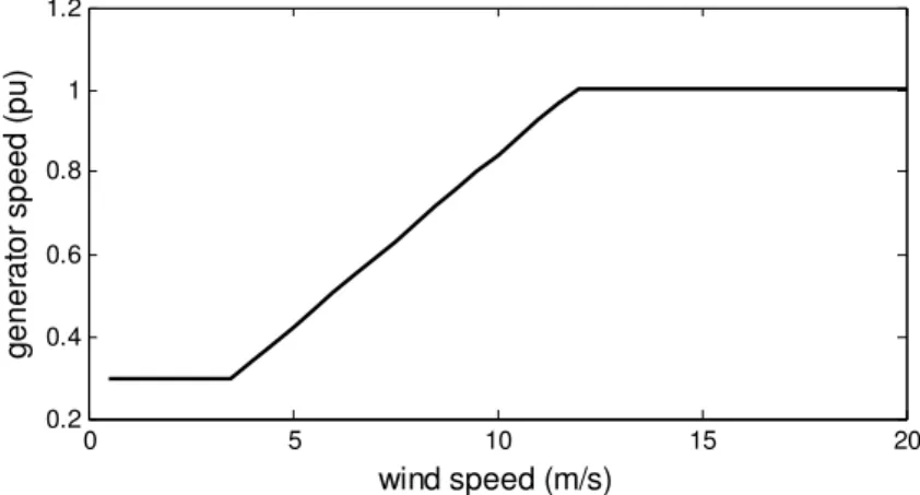
For wind speed belong 11,8 m/s, the rotor speed assumes different values in order to achieve the
optimal speed to maximize the power capture from the wind (Fig. 12). Above the nominal speed in
steady-state operation, the rotor is maintained at fixed velocity. The blade pitch angle control and the
0 5 10 15 20 0.2
0.4 0.6 0.8 1 1.2
wind speed (m/s)
g
e
n
e
ra
to
r
s
p
e
e
d
(
p
u
)
Fig. 12 Generator optimized speed for different wind speed.
B. Dynamic Analysis during Wind Gust Perturbation
The second part of the dynamic analyzes determines the effect of wind gust perturbations over a
certain period when the wind turbine is operating at nominal speed. In this analysis, the implemented
speed control maintains the rotor speed in a fixed value during the wind gust perturbation. The blade
pitch angle control actuates to minimize the effect of the wind gust on the electric system. The signal
adopted to control the blade pitch angle is the generated electric power. This pitch angle control
strategy minimizes the fluctuations of electric power injected into the electric system. The wind gust
perturbation (shown in Fig. 13) has its average value equal to 16 m/s.
0 2 4 6 8 10
12 13 14 15 16 17 18
time(s)
w
in
d
s
p
e
e
d
(
m
/s
)
Fig. 13 Wind gust perturbation.
The rotor speed is kept constant by the rotor side converter, as shown in Fig. 14. The pitch angle
control actuates to compensate the wind speed variation. When the wind speed becomes higher than
the average value, the pitch angle also increases to diminish the power capture from the wind. The
actuation of the blade pitch angle is less efficient when the average wind speed is closer or lower than
the nominal wind speed (11,8 m/s). In Fig. 15, the variation of the pitch angle during the wind gust is
0 2 4 6 8 10 0.6
0.7 0.8 0.9 1 1.1
time (s)
ro
to
r
s
p
e
e
d
(
p
u
)
Fig. 14 Rotor speed during wind gust perturbation.
0 1 2 3 4 5 6 7 8 9 10
0 5 10 15
time (s)
b
la
d
e
p
it
c
h
a
n
g
le
(
º)
Fig. 15 Blade pitch angle during wind gust perturbation.
One can see in Fig. 16 that the injected electric power suffers the influence of the wind gust
perturbation. This fact can be explained considering the time response of the mechanical actuator used
to vary the blade angle, which adds a time delay between the control order and the effective actuation.
0 1 2 3 4 5 6 7 8 9 10
0 0.5 1 1.5
time (s)
e
le
c
tr
ic
p
o
w
e
r
(p
u
)
VI. CONCLUSIONS
The methodology presented in this paper combines a 3D finite element model and an aerodynamic
model of a wind turbine. Using this methodology the dynamic simulations of the TFG can be
performed with accuracy avoiding the critical full 3D model. The dynamic simulations have showed
appropriate and accurate results for steady-state and dynamic characteristics of the wind turbine based
on TFG. The development of a full wind farm expanded model to analyze the impact on the offshore
transmission systems would give basis to compare its performance with other technologies.
APPENDIX
The authors gratefully acknowledge the financial support from Brazil by FAPESP (“Fundação de
Amparo à Pesquisa do Estado de São Paulo”), by CNPq (“Conselho Nacional de Desenvolvimento
Científico e Tecnológico”) and CAPES (“Coordenação de Aperfeiçoamento de Pessoal de Nível
Superior”) and also from Germany by DAAD (“Deutscher Akademischer Austausch Dienst”) to
develop this research. The authors also acknowledge Doctor Rolf Blissenbach for the cooperation and
the technical discussions.
REFERENCES
[1] Global Wind Energy Council, “Global Wind 2009 Report”, 2009.
[2] T. Ackermann, “Wind Power in Power Systems”, John Wiley & Son, England, 2005. [3] European Wind Energy Association, “Wind Energy - The Facts”, March, 2009.
[4] M. R. Dubois, “Optimized Permanent Magnet Generator Topologies for Direct-Drive Wind Turbines”, PhD thesis, Delft University of Technology, Delft, The Netherlands, 2004.
[5] H. Polinder, F. FA van der Pijl, Gert-Jan de Vilder, P. J Tavner, “Comparison of direct-drive and geared generator concepts for wind turbines”, IEEE Trans. on Energy Conversion, vol. 21, no. 3, pp. 725-733, 2006.
[6] D. Svechkarenko, “On Analytical Modeling and Design of a Novel Transverse Flux Generator for Offshore Wind Turbines”, Licenciature thesis, The Royal Institute of Technology - KTH, Sweden, 2007.
[7] Ioan-Adrian Viorel, G. Henneberger, R. Blissenbach, Lars Löwenstein, “Transverse Flux Machines – Their behavior, design, control and applications”, Mediamira, Romania, 2003.
[8] M. R. Dubois, H. Polinder, “Study of TFPM machines with toothed rotor applied to direct-drive generators for wind turbines”, Nordic Workshop on Power and Industrial Electronics, Norway, 2004.
[9] R. Blissenbach, G. Henneberger, “Numerical calculation of 3D eddy current fields in transverse flux machines with time stepping procedures”, The International Journal for Computation and Mathematics in Electrical and Electronic Engineering - COMPEL, vol. 20, No. 1, pp. 152-166, 2001.
[10]Joao S. D. Garcia, Mauricio V. Ferreira da Luz, Joao Pedro A. Bastos, and Nelson Sadowski , “Transverse Flux Machines: What for?” , IEEE Multidisciplinary Engineering Education Magazine, vol. 2, no.1, pp. 4-6, 2007.
[11]J. G. Slootweg, H. Polinder, W. L. Kling, “Representing Wind Turbine Electrical Generating Systems in Fundamental Frequency Simulations”, IEEE Trans. on Energy Conversion, vol. 18, no.4, pp. 516–524, 2003.
[12]M.N. Uddin, T.S. Radwan, G.H. George, M.A. Rahman, “Performance of current controllers for VSI-fed IPMSM drive”, IEEE Transactions on Industry Applications, vol. 36, no.5, pp. 1531–1538, 2000.