Revista Brasileira de Estudos Regionais e Urbanos (RBERU) Vol. 05, n. 1, pp. 61-73, 2011
http://www.revistaaber.org.br
LOCATION OF SUGAR CANE PRODUCTION AND FUEL DEMAND IN BRAZIL Gervásio Ferreira dos Santos
Doutor em Economia FEA/USP
Professor e Pesquisador do Departamento de Economia e PPGE/UFBA. E-mail: [email protected]
RESUMO: O objetivo deste trabalho é avaliar as diferenças regionais no comportamento do consumidor de combustível no Brasil induzidas pela produção regional de etanol no país. Da mesma forma que várias atividades econômicas no Brasil, as plantações de cana-de-açúcar e, consequentemente, a produção de etanol, são espacialmente concentradas. A hipótese do trabalho é que as diferenças regionais do nível de renda, de produtividade na produção de etanol e os custos de transporte podem afetar a competitividade dos combustíveis entre os estados brasileiros. Por este motivo, o conhecimento de como a localização da produção de etanol afeta o comportamento do consumidor pode auxiliar na compreensão de possíveis impactos da política energética nacional sobre a diversificação de combustíveis nas regiões. Nesse sentido, foram realizadas estimações econométricas de equações de demanda por etanol e gasolina utilizando um modelo de painel dinâmico. Em seguida, variáveis binárias de interação foram usadas para avaliar como as equações de demanda divergem entre as regiões consideradas como maiores e menores produtores de etanol no Brasil. Os resultados mostram que existem ganhos consideráveis para os consumidores de etanol e gasolina nas maiores regiões produtoras de etanol do país.
Palavras-chave: Localização; Plantações de Cana-de-Açúcar, Etanol, Demanda de Combustíveis.
Classificação JEL: Q41; R12; D12
ABSTRACT: The objective of this paper is to evaluate the regional differences in the fuel consumer’s behavior induced by regional production of ethanol in Brazil. In the same way that other economic activities in Brazil, the sugar cane plantations and consequently the ethanol production, are spatially concentrated. The hypothesis of the paper is that regional differences of the income level, productivity in the ethanol production, and transport costs may affect competitiveness of the fuels among Brazilian states. For this reason, the knowledge of how the location of ethanol production affects consumer’s behavior might bring some insights about the possible impacts of the national energy policy regarding the fuel diversification. Econometric estimation of demand equations for ethanol and gasoline will be carried using a dynamic panel model. After that, binary interaction variables will be used to evaluate how the demand equations diverge between the largest and smallest ethanol producers’ regions in Brazil. The results show that there might be considerable gains for the ethanol and gasoline consumers in largest ethanol producer regions.
Key words: Location; Sugar cane plantations, Ethanol, Fuel demand.
1. Introduction
The fuel diversification in the Brazilian fuel market is well known in the international energy economics literature. This diversification is highlighted because of the use of ethanol in large scale in the market and strongly competing with gasoline. For this reason, there are four main fuels in this market: gasoline, ethanol, compressed (vehicular) natural gas (CNG), and diesel. Santos (2011) points out that ethanol has played a historic role in the national energy policy, being an important alternative in period of high oil prices or to face environmental enforcements. In addition, CNG has been introduced in the market and also competes with ethanol and gasoline. In this diversified marked, new market rules and technological advances in the automobile industry such as flex-fuel engines are increasing the competition between fuels. For this reason, consumers are becoming more prices sensitive and adjusting faster towards desired demand levels.
Because of the rainfall conditions and quality of land, the sugar cane plantations are considerably concentrated in the Center South region of Brazil. For this reason, transport costs, productivity differentials and historical income concentration in the Brazilian economy can make fuel consumption to be heterogeneous in space. The question that emerged is: how different is the consumer behavior in the largest compared to the smallest sugar cane producers regions in Brazil? To give an answer for this question, the present study is designed to make the econometric estimation of fuel demand equations for ethanol and gasoline using a dynamic panel data model. After that, binary (dummy) interaction variables will be used to evaluate differences in demand equations between the largest and smallest sugar cane producers regions.
The following Section presents the main elements of the Brazilian fuel market. In the Section Three the spatial aspects of sugar cane plantations and ethanol price differentials between the largest and smallest ethanol producers regions are presented. Section Four presents the econometric specification to estimate demand equations for ethanol and gasoline. In the Section Five the data requirements are described. The results will be presented in Section Six. Finally, in the Section Seven, some final remarks are discussed.
2. Fuel Diversification in Brazil
The dynamics of the Brazilian fuel and its liberalization process started in 1997, when the known Law of Petroleum (Law 9.478/97) was introduced. In addition, new designs for the energy policy and the competition were introduced in the fuel market through the free prices and free entry to new agents. The impact of this policy on the market with a considerable diversity of substitute and complementary fuels has dramatically changed the structure of fuel demand in Brazil. The Brazilian fuel market is considerably competitive because of the presence of many fuel distribution companies associated with the fuel diversification and, technological advances in the automobile industry such as the introduction of the flex-fuel engines and the use of ethanol in large scale. For Santos (2011), the dynamic of the Brazilian fuel market is centered on the ethanol demand, mainly after the introduction of the flex-fuel engine technology. The knowledge of how the location of sugar cane plantations affects the fuel demand might provide important insights about the future directions of energy policy. In order to comprehend the role of ethanol in the Brazilian market fuel it is necessary to understand the cycle from the introduction of ethanol to the spatial distribution sugar cane plantations nowadays, considering that local features of consumers and transport costs may determine regional differences in price and income elasticity of demand.
According to Santos (2011), the use of ethanol in the Brazilian fuel market was introduced in the country in 1975. Because of the oil shocks in 1974 and 1979, local government implemented an energy policy designed to introduce the fuel ethanol in the energy matrix of the country, through the Pro Alcool or National Program of Alcohol. The program was a large scale energy production program designed to substitute vehicular fossil fuel with ethanol produced from sugar cane. The international conjuncture favoured the implementation of this energy policy, because further the high
oil prices the low sugar prices in the international commodity market at that time was determinative to convert the use of sugar cane from sugar to ethanol.
Regulation policy in the fuel market jointly to agreements with the local automobile industry were important for the success this policy. Ethanol fuel was massively introduced as a complementary and substitute fuel in Brazil. The chemical structure of ethanol allows it to be mixed into gasoline. For this reason, it may assume the features of a complementary good to gasoline. So, the government determined the mixture of 22% of ethanol in the commercial gasoline. Nowadays, this mixing still remains about to 25%, according to the National Agency of Oil and Biofuel -ANP (2008). In addition, an agreement with the Brazilian automobile industry allowed the production of vehicles with engines that use only ethanol. These policies made that the Brazilian energy policy an important international benchmark for many years, mainly because of their contribution to environmental enforcements.
The use of ethanol in the fuel market was very important to Brazil until the first half of the 1980’s. After this period, its use started to decline. The main reason for this decline was the decline of oil prices and, consequently, the same movement in the price of oil derivatives such as gasoline. On the other hand, the increase of sugar prices in the international market also makes it difficult to maintain the program. In addition to this unfavourable international conjuncture, the local conjuncture pushes the Brazilian economy to liberal policies which pressed the elimination of subsidies for the program. In face of these problems, the use of ethanol in Brazil declined considerably. For this reason, the production of ethanol and vehicles with ethanol engines was reduced to a small and residual scale in the country until the beginning of 2000’s. Because of calorific value of ethanol to be smaller than gasoline, the competitiveness of ethanol depends on the maintenance of its price about to 70% of the gasoline price in the fuel market. For this reason, since 1989, when the Pro Alcohol collapsed and this percentage was higher than 75%, the Brazilian government has applied policies to maintain the price relation around 70% using, slightly handling fuel taxes. Since that time, to subsidize ethanol and CNG, the tax named Contribution of Economic Domain (CIDE) has not been charged on these two fuels.
Figure 1 – Price relations in the Brazilian fuel market – (Jul/2001-Dec/2007)
Source: ANP – Brazilian National Agency of Oil and Biofuel.
Despite the decline in the use of ethanol after the end of 1980’s, a considerable fleet consuming ethanol still remained in the fuel market. The National Department of Transport accounted that in 2006 the national fleet was composed of 45.6 million vehicles. From this amount, 3.0 million was pumped just with ethanol, which represented 13.6% of the light vehicle fleet of 22.0 million.
0 0.1 0.2 0.3 0.4 0.5 0.6 0.7 0.8 ju l/ 0 1 o u t/ 0 1 ja n /0 2 ab r/ 0 2 ju l/ 0 2 o u t/ 0 2 ja n /0 3 ab r/ 0 3 ju l/ 0 3 o u t/ 0 3 ja n /0 4 ab r/ 0 4 ju l/ 0 4 o u t/ 0 4 ja n /0 5 ab r/ 0 5 ju l/ 0 5 o u t/ 0 5 ja n /0 6 ab r/ 0 6 ju l/ 0 6 o u t/ 0 6 ja n /0 7 ab r/ 0 7 ju l/ 0 7 o u t/ 0 7 Ethanol/Gasoline GNV/Gasoline
This stock of vehicles pumped with ethanol was important to maintain the developments in the technology of production of both ethanol and engines that use ethanol. In 1990’s the federal government started to introduce CNG in the fuel market as a substitute for diesel in large road vehicles in the large urban centers, specifically in Sao Paulo and Rio de Janeiro by reducing tax on property of automotive vehicles of vehicles that used the respective fuel. After that, this fuel started to compete with gasoline and ethanol in other regions of the country and, in 2007, 1.5 million vehicles was using CNG, according to the Brazilian National Institute of Oil and Gas (2008).
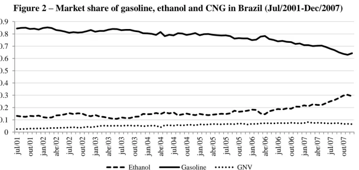
The CNG is mainly used in used vehicles, because the Brazilian automobile industry does not produce light vehicles with engines using CNG. For this reason, a conversion process is necessary to implement a second fuel tank in the vehicle and consumers may pump with a second fuel (gasoline or ethanol) in addition to CNG. The government subsidizes on CNG consolidated it the fuel market. The importance of CNG is associated with the expansion of the fuel diversification in the market for light vehicles, which become the consumer more prices sensitive. According to Figure 2, gasoline still remained as the main fuel used in light vehicles in Brazil. However, the market share declined from 84.4% in 2001 to 64.2% at the end of 2007. On the other hand, the use of ethanol increased from 13.2% to 29.3% and CNG from 2.5% to 6.5%.
Figure 2 – Market share of gasoline, ethanol and CNG in Brazil (Jul/2001-Dec/2007)
Source: ANP – National Agency of Oil and Biofuel.
The evolution of events that increased the fuel diversification in Brazil recently had the contribution of an important revolution in the automobile industry. This revolution came with the use of flex-fuel engine technology by the car makers. The technology allows using gasoline, ethanol or CNG (this later in a small scale) to work the engine. According to Santos (2011), the flex-fuel engines were developed in the United States in the 1980’s and was tried in Brazil since the 1990’s and finally in introduced in the country by the car makers in 2003. Because of this technology, the sales of vehicles with ethanol plus flex-fuel engines overcame those with gasoline engines. In 2007, the sales of flex-fuel vehicles represented 73.8%, according to Figure 3, which totalled 1.83 million units. The remaining sales were divided into 8.1% to only ethanol engines, 9.8% goes gasoline and 8.5% for diesel. 0 0.1 0.2 0.3 0.4 0.5 0.6 0.7 0.8 0.9 jul /01 out/ 01 jan/02 abr /02 jul/02 out/ 02 jan/03 abr /03 jul /03 out/ 03 jan/04 abr /04 jul /04 out/ 04 jan/05 abr /05 jul /05 out/ 05 ja n/06 abr /06 jul /06 out/ 06 jan/07 abr /07 jul /07 out/07 Ethanol Gasoline GNV
Figure 3 – Retail sales (quantity of vehicles) in Brazil by type of fuel (Jan/99 – Dec/07)
Source: Anfavea – Brazil's National Association of Vehicle Manufacturers
The question that emerges to face the trend of evolution in the diversification process of in the fuel market is that the important share of ethanol in the national market might determine different consumer behaviour in the regions. This might happen because the regional production and productivity of ethanol is not homogeneous in the whole country. Because of CNG has no significant share of the fuel market yet, the dynamics of the Brazilian fuel market is centered on the changes in the ethanol and its competition with gasoline. In order to investigate this problem, this paper explores some features of spatial distribution of sugar cane plantations in Brazil, jointly with ethanol price differentials to analyse the importance of this issue for the competition in the fuel market. These elements will be described in the next section.
3. Spatial distribution of sugar cane plantations in Brazil
The sugar cane plantation area in Brazil was about 7.09 million hectares of land in the harvest 2007/2008. In this area, it was produced 493.3 million tons of sugar cane. This sugar cane resulted in the production of 141.4 million barrels of ethanol and 30.7 million tons of sugar. The ethanol production might be splitted in 36.4% of ethanol anidre usually used to be mixed with gasoline, and 63.6% of ethanol hydrated that is used as substituted fuel to gasoline. Apart from the considerable amount of sugar cane produced in Brazil, some factors, such as land fertility and rainfall level, makes the production extremely concentrated in the national territory.
0 0.1 0.2 0.3 0.4 0.5 0.6 0.7 0.8 0.9 1 jan/99 mai/99 set/ 99 jan/00 mai/00 set/ 00 ja n/01 mai/01 se t/ 01 jan/02 mai/02 set/ 02 jan/03 mai/03 set/ 03 jan/04 mai/04 set/ 04 jan/05 mai/05 set/ 05 jan/06 mai/06 set/ 06 jan/07 mai/07 set/ 07
Figure 4 - Sugar cane and ethanol production in the Brazilian states (% share) in 2007
Source: Brazilian Institute of Geography and Statistics
Figure 4 shows the distribution of sugar cane production in Brazil in the harvest 2007/2008. The production is concentrated in the Center-South states, which produced 87.4% (431.1 million tons) of the national production in this period. The São Paulo state is the largest producer. This state produces 60.1% (296.3 million tons) of the national production. The North-Northeast regions produce 12.6% of the national production and this production is concentrated in the states of Pernambuco and Alagoas, which jointly produce 9.5% of the national production.
Figure 5 - Sugar cane production clusters in Brazil in 2007
Source: Brazilian Institute of Geography and Statistics 0.00% 10.00% 20.00% 30.00% 40.00% 50.00% 60.00% 70.00% A cre A ma p á Ro n d ô n ia Ro ra ima A ma zo n as Pará T o can ti n s Maran h ão Pi au í Ceará Ri o G ran d e d o N o rt e Paraí b a Pe rn amb u co A lag o as Se rg ip e Bah ia Mi n as G erai s E sp íri to San to Ri o d e Ja n ei ro São Pau lo Paran á San ta Carat in a Ri o G ran d e d o Su l Mat o G ro ss o Mat o G ro ss o d o Su l G o iá s
Ethanol Sugar Cane Production
Center-South North-Northeast
The spatial aspects of sugar cane production were evaluated through the Moran Index and Local Indicator of Spatial Association (Lisa), using data for the 558 Brazilian micro-regions. The significant Moran Index of 0.61 indicated the presence of spatial autocorrelation in the sugar cane production. The Lisa indicator is plotted in the Figure 5. As can be seen, there are two important clusters of sugar cane production in the Brazilian economy. The largest is located in the Center-South region, around the State of São Paulo. The second is located in the Northeast region and is composed by the states of Pernambuco and Alagoas.
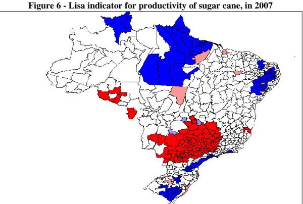
Because of the ethanol production is directly related to the sugar cane production, the spatial concentration might bring some implications for the ethanol prices in the Brazilian territory. The Figure 6 shows the Lisa indicator for the variable productivity of sugar cane (production/hectare) in the Brazilian micro-regions. As can be seen, there are three significant productivity clusters of sugar cane in Brazil, all of them in the Center-South region. Figure 6: Sugar cane productivity clusters in Brazil in 2007.
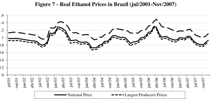
From the Figures 5 and 6 it might be extracted the fact that the most productive regions also are the most productive. When this fact is associated with transport costs, and assuming that the technology to produce ethanol from sugar cane is the same in Brazil, prices differentials might emerge in the economic space. The Figure 7 shows the real prices to final consumers of the fuel ethanol in Brazil for the eight largest producer states (São Paulo, Paraná, Minas Gerais, Mato Grosso, Mato Grosso do Sul, Goiás, Paernambuco e Alagoas) and in the smallest producers (the other 19 states).
Figure 6 - Lisa indicator for productivity of sugar cane, in 2007
Figure 7 - Real Ethanol Prices in Brazil (jul/2001-Nov/2007)
Source: National Agency of Oil
As can be seen, the real prices in the smallest producer states are considerably above the national prizes. On the other hand, the real prices in the largest producer states are slightly below the nations prices. This evidence suggests that the consumer behaviour might differ regarding price changes in the ethanol, gasoline or CNG. To evaluate this behaviour econometric estimation of demand equations for ethanol and gasoline will be done using a dynamic panel data model.
4. Econometric Specification Empirical Strategy
The main papers about estimation of fuel demand equations in the energy economics literature related to gasoline demand. In the most influential papers of Energy Economics, Dahl and Sterner (1991) summarize a set of principles, models and data requirements used for estimation of gasoline demand. Although restricted to time series data, others like Ramanathan (1999), Eltony and Al-Mutairi (1995), and Bentzen (1994) provide good insights about the subject.
The seminal studies in Brazil regarding to gasoline and ethanol are those of Burnquist and Bacchi (2002), Alves and Bueno (2003), Roppa (2005). These authors estimated the demand equations for gasoline for different fuels using year time series and found different conclusions. In general, the conclusions were the fuel that demand is more sensitive to income than price in the short and in the long-run, and the ethanol is an imperfect substitute for gasoline even in the long-run. A different research was conducted by Iootty (2004) that compared the competitiveness between gasoline and CNG. The author found that CNG is an imperfect substitute for gasoline and the demand for CNG was price inelastic. Despite the importance of these researches the specification using time series might be improved due to the availability of data to Brazil. In doing so, Santos (2011), estimated a set of price and income elasticity’s for gasoline, ethanol and CNG using panel data models. Further a detailed review of price and income elasticity’s of fuel demand in Brazil, the results confirmed the previous studies and improved the knowledge of competitiveness between gasoline, ethanol and CNG. The specifications for panel data were based on the classical studies of Balestra and Nerlove (1966), Baltagi and Griffin (1983), Hsaio (1985 and 1986), Baltagi (2001).
For this reason, the specification considers that the demand is technologically dependent on the vehicles’ engine. It will be considered first a market without flex-fuel engines due to large previous stock of non-flexible engines. The basic assumption is that consumers have some difficulty in changing to another fuel in the short-run and in the long-run. Therefore, previews consumption determines the pattern of consumption in the present. This modelling allows the estimation of the speed of adjustment of the consumers regarding the desired demand levels.
0 0.2 0.4 0.6 0.8 1 1.2 1.4 1.6 ju l/ 0 1 o u t/ 0 1 ja n /0 2 ab r/ 0 2 ju l/ 0 2 o u t/ 0 2 ja n /0 3 ab r/ 0 3 ju l/ 0 3 o u t/ 0 3 ja n /0 4 ab r/ 0 4 ju l/ 0 4 o u t/ 0 4 ja n /0 5 ab r/ 0 5 ju l/ 0 5 o u t/ 0 5 ja n /0 6 ab r/ 0 6 ju l/ 0 6 o u t/ 0 6 ja n /0 7 ab r/ 0 7 ju l/ 0 7 o u t/ 0 7
The specification used in the present study is the same of Santos (2011), the partial adjustment model of (Pesarin and Smith, 1995), as can be seen in equation (1)
) , , , ( ( ) ( ) 1 git sit it it it f p p I y y (1)
In this equation, the indexes i and t represents the region i and period t. regarding the variables, yit represents the per capita fuel demand, p(g)it is the respective price, p (g)it is the real price of substitute good, it is the real per capita income, and yit-1 is the time lagged per capita fuel demand. This model follows Dahl and Sterner (1991). However, the lagged dependent variable captures the inertia of economic behavior, based on assumptions of partial adjustments or adaptive expectations. For details of this specification, see Santos (2011) and Liu (2004).
Based on equation (1), the equations to be estimated are:
) ( ) ( ) ( 4 ) ( 3 ) ( 2 ) ( 1 ) 1 ( 0 ) ( ln ln ln ln ln lnGit Git PGit PEit PGNVit GDPit i uit (2) ) ( ) ( ) ( 4 ) ( 3 ) ( 2 ) ( 1 ) 1 ( 0 ) ( ln ln ln ln ln lnEit Eit PGit PEit PGNVit GDPit i uit (3)
In the equations (2) and (3), the two dependent variables will be per capita consumption of gasoline (G), ethanol (E) and CNG. The other explanatory variables are, respectively, the real prices of gasoline (PG), ethanol (PE) and CNG (PCNG), and per capita Gross Domestic Product (GDP). The lagged dependent variable might improves the fit of models, mainly because non-existence of a variable representing to variation in vehicle stock. Besides that, it also allows to estimate the speed of adjustment of the respective demand through the estimation of the parameter θ = (1 -γ), according to Santos (2011) and Liu (2004). Considering the specification for panel data in (2) and (3), it is assumed an unobserved time invariant region-specific fixed effect μi. This term represents the local heterogeneity that affects the fuel demand. In doing so, we might capture regional differences in the parameter derived only from regional differences in the behaviour of regional consumers.
The final consideration regarding the empirical strategy is the fact that since y(it) is in function μi and y(it-1) also is in function of μi that is supposed to be fixed over time. For this reason, an endogeneity problem must be considered in the estimation, even the remainder error term is not serially correlated, see Nickell (1981). Thus the Pooled (OLS), Fixed and Random Effect estimators would be biased and inconsistent. Our strategy was to use the GMM estimator from Arellano and Bond (1991), based on Anderson and Hsaio (1981 and 1982) and presented in Baltagi (2001) and Wooldridge (2004). This estimator generates consistent estimates when the panel or time units tend to infinity and, also eliminates the unobserved fixed effect.
For the estimation of the equations (2) and (3), a panel monthly dataset regarding 27 Brazilian states for the period from Jul/2001 to Dec/2007 was built using data from ANP. After eliminating regions with no data about CNG, the sample was reduced to 15 states. The monthly price index and population data were obtained from the Brazilian Institute of Geography and Statistics (IBGE). A proxy variable of Tax on Trade of Products and Services (ICMS), from the Brazilian National Treasury, was used to capture the statistical variation in the monthly GDP. This variable is net from the ICMS that is charged on fuel.
5. Results and comparisons
Based on equations (2) and (3), estimated on logarithm the estimation using One-step GMM, which provides the adjustment coefficients, price, cross-price and income elasticities. After that, to evaluate the sensitivity of consumers regarding the location of ethanol production, it was introduced multiplicative dummy variables for interaction between ethanol prices and the panel units representing the eight largest ethanol producers (Brazilian States). O objective was to evaluate if the
price and cross price elasticity of ethanol demand are different in the markets which also are large ethanol producers.
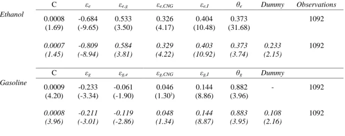
Table 1 - One-step GMM-Arellano-Bond short-run estimations of fuel demand equations for Brazil
C εe εe,g εe,CNG εe,I θe Dummy Observations Ethanol
0.0008 -0.684 0.533 0.326 0.404 0.373 1092
(1.69) (-9.65) (3.50) (4.17) (10.48) (31.68)
0.0007 -0.809 0.584 0.329 0.403 0.373 0.233 1092
(1.45) (-8.94) (3.81) (4.22) (10.92) (3.74) (2.15)
C εg εg,e εg,CNG εg,I θg Dummy Gasoline
0.0009 -0.233 -0.061 0.046 0.144 0.882 - 1092
(4.20) (-3.34) (-1.90) (1.30)) (8.86) (3.96)
0.0008 -0.211 -0.119 0.048 0.144 0.883 0.108 1092
(3.96) (-3.01) (-2.86) (1.34) (8.87) (3.95) (2.16)
Note: The values in brackets refer to z statistics.
Table 1 presents the one-step GMM estimations for the elasticities ε(.), the cross-price elasticities ε(.,.), and adjustment coefficients θ(.) regarding the demand equations by ethanol and gasoline. For each equation the Sargan test suggested to reject the hypothesis of over-identification restriction for one step estimation. The Arellano-Bond test also suggested rejecting the hypothesis of no serial autocorrelation in residuals of order 1 but not to reject the hypothesis of no serial autocorrelation of order 2. This makes the dependent variables valid instrumental variables with at least two legs. Because the monthly data comprises a period of six years, the equations were estimated to obtain short-run estimations.
In general, the results in Table 01 show that all price elasticities were smaller than one, which is common for energy goods, marked by inelasticity of demand. In addition, all cross-price elasticities also were smaller than one, which characterize the three fuels as imperfect substitutes, for each other. Other results are described below.
Ethanol
The results of the first ethanol demand equation were supported by economic theory. Due to lacks of no previous estimation in the international literature, no comparison was possible. The negative and high price elasticity of -0.684 might be an evidence that ethanol consumers are from lower income groups more price sensitive and being attracted by cheaper fuel. On the other hand, this result might have reflected the introduction of flex-fuel engines in the market1. The cross-price elasticities regarding gasoline and CNG had and expected positive sign. The high cross-price elasticity regarding gasoline price of 0.533 implies that ethanol competes considerably with gasoline. It also suggests that the gasoline prices are more important for ethanol demand than gasoline demand. Similarly, the cross-price elasticity regarding CNG of 0.326 also implies that ethanol already competes with CNG. The income elasticity of 0.404, considerably greater than that from gasoline demand, also is an evidence that ethanol consumers belong to lower income groups. At last, the adjustment coefficient of 0.373 suggests that ethanol consumers are distant from desired demand level, i.e., the ethanol market has a strong potential to rapidly increase in Brazil.
In the second ethanol demand equation the dummy interaction shows that there is an interaction statistically significant between the eight largest ethanol producer states and the ethanol prices of 0.233. This positive interaction makes that the price elasticity of ethanol demand of the consumers belonging to the largest ethanol producer states decrease to 0.577, which is the sum of -0.810 plus 0.233. This elasticity is considerably smaller than the price elasticity of --0.810 of the smallest producer regions. This shows that in the largest ethanol producer regions the consumers are less sensitive to ethanol prices. This might promote gains for the producers and consumers in these regions. On the other hand, it also might be evidence that transport cost contribute negatively to the ethanol demand in the smallest producers regions than in the largest producers and the productivity differentials contribute positively to largest producers regions.
Gasoline
For the results of the first gasoline demand equation, the price-elasticity of -0.233 had the expected sign and is close to Burnquist and Bacchi (2002) estimation of -0.319. This result also is considerably close to that of Dahl and Sterner (1991). The cross-price elasticity of ethanol of -0.061 had an unexpected sign and was not close to others estimations for Brazil. However, the persistence of this negative sign also is verified in others studies such as Alves and Bueno (2003) and Roppa (2005). This suggests the hypothesis that ethanol might be considered a complementary good to gasoline. Because of the fact that gasoline is composed of 25% of ethanol and also due the high statistical significance of the parameter, this hypothesis might be confirmed. On the other hand, the cross-price elasticity regarding CNG of 0.046 had expected sign but not so statistically significant; there is no estimative in the literature to be compared. The income elasticity of 0.144 was close to Roppa (2005) and Iootty (2004). This small value might be explained by the fact that gasoline consumers are from higher income groups in Brazil.
The adjustment coefficient of 0.882 is close to one and indicates that in the short-run the demand for gasoline is close to desire demand level. This means that the main explanatory variable of gasoline demand variation might be only the large (and older) stock of vehicles with gasoline engines.
In the second equation, the dummy interaction between ethanol prices the eight largest ethanol producer states also was statistically significant of 0.108. This positive interaction makes that cross-price elasticity of gasoline demand regarding the ethanol cross-prices decrease to -0.011, which is the sum of -0.119 plus 0.108. This cross-price elasticity is smaller than the cross-price elasticity of -0.119 810 of the smallest producer regions. This means that the gasoline consumers located in the largest ethanol producer states are less sensitive to ethanol prices, relatively to other regions. In the same way that for ethanol consumers, this might be an evidence of possible relative gains for producers and consumers derived from differentials of transport cost e productivity of ethanol.
5. Final Remarks
This paper proposed to evaluate the regional differences in the fuel consumer’s behavior induced by regional production of ethanol in Brazil. Our hypothesis was that the regional differences in the income, productivity of ethanol and transport costs affected competitiveness of the fuels among Brazilian states. Econometric estimation of demand equations for ethanol and gasoline were developed using a dynamic panel model and binary interaction variables to evaluate how the demand equations diverge between the largest and smallest ethanol producers’ states in Brazil.
The results showed that ethanol and gasoline are imperfect substitutes and complementary goods. The adjustment coefficient also showed that ethanol demand is more distant from the desired demand level than gasoline. Regarding regional differences in the consumer behavior, in the largest ethanol producers states the ethanol consumers are less sensitive to ethanol price variations. Due the fact that ethanol might be considered a complementary good to gasoline, the gasoline consumers also
is less sensitive to ethanol price variations in the largest ethanol producers regions. For this reason, there might be considerable gains for the ethanol and gasoline consumers in this regions explained by the production systems and location of sugar cane plantations.
Finally, despite of the fact that there is some difficulty to organize a dataset for the Brazilian micro-regions, advances might be achieved handling the regional differentials in the gasoline prices and/or using spatial panel data econometrics.
References
Anderson, T. W.; Hsaio, C. Estimation of dynamic models with error components. Journal of the American Statistical Association, v. 76, n. 375, p. 598-606, 1981.
Anderson, T. W.; Hsaio, C. Formulation and estimation of dynamic models using panel data. Journal of Econometrics, v. 18, n. 1, p. 47-82, 1982.
Arellano, M.; Bond, S. Some tests of specification for panel data: Monte Carlo evidence and an application to employment equations. Review of Economic Studies, v. 58, n. 2, 277-297, 1991. Balestra, P.; Nerlove, M. Pooling cross-section and time-series data in the estimation of a dynamic
model: The demand for natural gas. Econometrica, v. 34, n. 3, p. 585-612, 1996.
Baltagi, B. H. Econometric Analysis of Panel Data. Chichester: John Wiley and Sons, 2001.
Baltagi, B. H.; Griffin, J. M. Gasoline demand in the OECD: An application of pooling and testing procedures. European Economic Review, v. 22, n. 2, p. 117-137, 1983.
Bentzen, J. An empirical analysis of gasoline demand in Denmark using cointegration techniques. Energy Economics, v. 16, n. 2, p. 39-143,1994.
Brazilian Institute of Geography and Statistic (IBGE). Índices de preços e estimativas populacionais. Available at http://www.ibge.gov.br.
Brazilian National Treasury. Arrecadação mensal dos estados. Available at http://www.receita.fazenda.gov.br.
Bueno, R.; Silveira, A. Short-run, Long-run and Cross Elasticities of Gasoline Demand in Brazil. Energy Economics, v. 25, n. 2, p. 191-1999, 2003.
Burnquist H. L.; Bacchi, M. R. P. A demanda por gasolina no Brasil: uma análise utilizando técnicas
de co-integração, 2002. (Discussion paper) Available at
www.cepea.esalq.usp.br/pdf/DemandaGasolina.pdf.
Dahl, C.; Sterner, T. Analyzing gasoline demand elasticities: a survey. Energy Economics, v. 13, n. 3, p. 203-210, 1991.
Eltony, M. N.; Al-Mutairi, N. H. Demand for gasoline in Kuwait: an empirical analysis using co-integration techniques. Energy Economics, v. 17, n. 3, p. 249–253, 1995.
Hsaio, C. Analysis of Panel Data. Cambridge University Press: Cambridge, 1986.
Iootty, M. et al. Uma análise da competitividade preço do CNG frente à gasolina: estimação das elasticidades da demanda por CNG no Brasil no período recente”. In Rio Oil and Gas Expo and Conference, edited by IE/UFRJ. UFRJ: Rio de Janeiro, 2004.
Liu, G. Estimating Energy Demand Elasticities for OECD Countries: a dynamic panel data approach. Statistics Norway, 2004. (Discussion paper n. 373). Available at http://www.ssb.no/publikasjoner/DP/pdf/dp373.pdf
National Agency of Oil and Biofuel (ANP). Levantamento mensal de preços e vendas de combustíveis no Brasil, 2008. Available at http://www.anp.gov.br.
National Department of Transit (DENATRAN). Frota nacional de veiculos automotres. Available at www.denatran.gov.br.
Nickell, S. Biases in dynamic models with fixed effects. Econometrica, v. 49, n. 6, p. 1417-1426, 1981.
Pesarin, M. H.; Smith, R. Estimating long-run relationships from dynamic heterogeneous panels. Journal of Econometrics, v. 68, n. 1, p. 79-113, 1995.
Ramanathan, R. Short and long-run elasticities of gasoline demand in India: an empirical analysis using co-integration techniques. Energy Economics, v. 21, n. 4, p. 321-330, 1999.
Roppa, B. F. Evolução do consumo de gasolina no Brasil e suas elasticidades: 1973 a 2003. UFRJ: Rio de Janeiro, 2005.
Santos, G. F. Fuel Demand in Brazil in a Dynamic Panel Data Approach. Energy Economics, 2011. Forthcoming.