Impact of in-band crosstalk on the performance of optical coherent detection communication systems

(1)

D

EPARTMENT OF INFORMATION SCIENCE AND TECHNOLOGY

Impact of In-Band Crosstalk on the Performance of

Optical Coherent Detection Communication Systems

Dissertation presented in partial fulfillment of the requirements for the Masters Degree on

Telecommunications and Information Science

by

Bruno Rafael Pereira Pinheiro

Supervisors:

Dr. João Rebola, Assistant Professor,

ISCTE-IUL

Dr. Luís Cancela, Assistant Professor,

ISCTE-IUL

(2)

(3)

(4)

(5)

Acknowledgements

I am fortunate to have been supervised in this dissertation by Prof. João Rebola and Prof. Luís Cancela. Throughout this work, their availability and patience in all my doubts and questions, provided me support and guidance to conclude this dissertation. I am also thankful to Instituto de Telecomunicações (IT) for providing access to their installations.

I would like to thank my family for their unconditional support, love and encouragement. A warm feeling towards Susana, who always helps me to get my confidence back when things became difficult.

Finally, I would like to thank all my friends and colleagues for all their support during the past years.

(6)

(7)

Resumo

A detecção óptica coerente leva à coexistência de sinais com diferentes formatos de modulação e diferentes ritmos binários nas redes ópticas. Devido a essa coexistência vários cenários de diafonia homódina (in-band crosstalk) são possíveis. Neste trabalho, o impacto do in-band crosstalk devido a sinais interferentes com o for-mato de modulação em amplitude em quadratura (M-QAM) no desempenho do PDM-QPSK e PDM-16-QAM receptores coerentes a um ritmo binário agregado de 100 Gbps é estudado utilizando simulação Monte-Carlo. A precisão do método de magnitude do vector de erro (EVM) também é investigado na presença de in-band crosstalk, e revelou ser suficientemente preciso na estimação o nível de interferência que leva a uma penalidade de 1 dB na relação sinal-ruído óptico (OSNR) no receptor. No entanto, a precisão do método EVM foi dimin-uída, relativamente à estimativa da penalidade na OSNR devido a níveis de in-band crosstalk mais elevados.

A influência do factor de duração de ciclo, do desalinhamento temporal e da diferença de fase entre o sinal interferência e o sinal seleccionado no desempenho do receptor é também avaliada. Mostra-se que o sinal QPSK com um factor de duração de ciclo de 33% é, em geral, o sinal seleccionado mais tolerante ao in-band crosstalk e o interferente menos prejudicial para o desempenho do receptor coerente. Mostramos também que o desalin-hamento temporal tem uma influência significativa no impacto do in-band crosstalk no desempenho do receptor coerente, quando o factor de duração de ciclo dos interferente ou do sinal seleccionado são baixos, e a diferença de fase tem impacto quase desprezável na variação da penalidade de OSNR.

Palavras-chave: Crosstalk homódino, magnitude do vector de erro, modulação de amplitude em quadratura, simulação de Monte-Carlo, sistemas ópticos com detecção coerente.

(8)

(9)

Abstract

Optical coherent technology leads to the coexistence of signals with different modulation formats and different bit rates in optical networks. Due to this coexistence several in-band crosstalk scenarios are possible. In this work, the impact of in-band crosstalk due to M-ary quadrature amplitude modulation (M-QAM) interferers on the performance of PDM-QPSK and PDM-16-QAM coherent receivers at an aggregated bit rate of 100 Gbps is studied using Monte Carlo simulation. The accuracy of the error vector magnitude method is also investigated in presence of in-band crosstalk and it revealed to be sufficiently accurate for the estimation of the crosstalk level that leads to a 1 dB Optical Signal-to-Noise ratio (OSNR) penalty at the receiver. However, the EVM method accuracy was diminished, concerning the estimation of the OSNR penalty due to higher crosstalk levels.

The influence of the duty-cycle, time misalignment and phase difference between interferers and selected signal on the receiver performance is also assessed. We show that the QPSK signal with a duty-cycle of 33% is, generally, the most tolerant selected signal to in-band crosstalk and the less detrimental interferer to the coher-ent receiver performance. We also show that the time misalignmcoher-ent has a significant influence on the in-band crosstalk impact, when the duty-cycles of the interferers or selected signal are low, and the phase difference has almost negligible impact on the OSNR penalty variation.

Keywords: Error vector magnitude, in-band crosstalk, Monte-Carlo simulation, optical coherent detection com-munication systems, quadrature amplitude modulation.

(10)

(11)

3 M-QAM Receiver Performance in Presence of ASE Noise 29 3.1 Introduction . . . 29 3.2 Optical Filtering . . . 29 3.2.1 Ideal Filter . . . 30 3.2.2 Super-Gaussian Filter . . . 30 3.3 Electrical Filtering . . . 31 3.3.1 Integrator-and-Dump Filter . . . 31 3.3.2 Bessel Filter . . . 32 3.4 System Validation . . . 33 3.4.1 DEC Method . . . 34 3.4.1.1 QPSK Modulation Format . . . 34

3.4.1.2 16-QAM modulation format . . . 36

3.4.1.3 64-QAM Modulation Format. . . 37

3.4.2 EVM Method . . . 40

3.5 Filters Optimization for the QPSK Modulation Format . . . 43

3.5.1 Gaussian Optical Filter and Fifth Order Bessel Electrical Filter . . . 44

3.5.2 Gaussian Optical Filter and Gaussian Electrical Filter . . . 47

3.5.3 Fourth Order Super-Gaussian Optical Filter and Fifth Order Bessel Electrical Filter . . . 49

3.5.4 Fourth Order Super-Gaussian Optical Filter and Gaussian Electrical Filter . . . 51

3.5.5 Best Filters Configuration for the QPSK Coherent Receiver . . . 53

3.6 Filters Optimization for the 16-QAM Modulation Format . . . 53

3.7 Conclusions . . . 56

4 M-QAM Receiver Performance in Presence of In-Band Crosstalk 59 4.1 Introduction . . . 59

4.2 In-Band Crosstalk Origin . . . 60

4.3 Crosstalk Simulation Model and Validation . . . 61

4.3.1 Simulation Model Description . . . 61

(13)

CONTENTS

4.4 QPSK Receiver Performance in Presence of In-band Crosstalk . . . 66

4.4.1 Different Modulation Format Orders . . . 67

4.4.1.1 Time Misalignment . . . 71

4.4.1.2 Phase Difference . . . 73

4.4.2 Same Modulation Format and Different Duty-Cycles . . . 75

4.4.2.1 Time Misalignment . . . 77

4.4.2.2 Phase Difference . . . 78

4.4.3 Mixed Modulation Formats and Different Bit Rates . . . 79

4.5 16-QAM Receiver Performance in Presence of In-band Crosstalk . . . 81

4.6 Conclusions . . . 85

5 Conclusions and Future Work 87 5.1 Final Conclusions . . . 87

5.2 Future Work . . . 89

(14)

(15)

List of Figures

1.1 Increase of the global IP traffic demands from 1985 to 2016 [1]. . . 1

1.2 Layering approach for a telecommunication network [3]. . . 2

1.3 Standards of the transport channel capacities and Ethernet port speeds [1]. . . 3

2.1 Schematic representations of the signal spectrum after the LO beating with the signal. . . 8

2.2 Time vector representation. . . 10

2.3 Frequency vector representation. . . 10

2.4 MC algorithm flow-chart. . . 11

2.5 Ideal IQ transmitter. . . 12

2.6 Ideal constellations for (a) QPSK, (b) 16-QAM and (c) 64-QAM mappings signals. . . 13

2.7 PSD of the simulated (a) 4-QAM, (b) 16-QAM and (c) 64-QAM signals. . . 14

2.8 Temporal representation of a (a) NRZ and (b) RZ with 50% duty-cycle pulse shapes and its respective PSDs, (c) and (d). . . 15

2.9 Schematic block diagram of a PDM coherent receiver with an optical quadrature frontend. . . . 16

2.10 Different configurations of a hybrid. . . 19

2.11 Directional coupler. . . 19

2.12 Mach-Zehnder interferometer . . . 21

2.13 Setup of a typical QF based on the configuration presented in Figure 2.9. . . 22

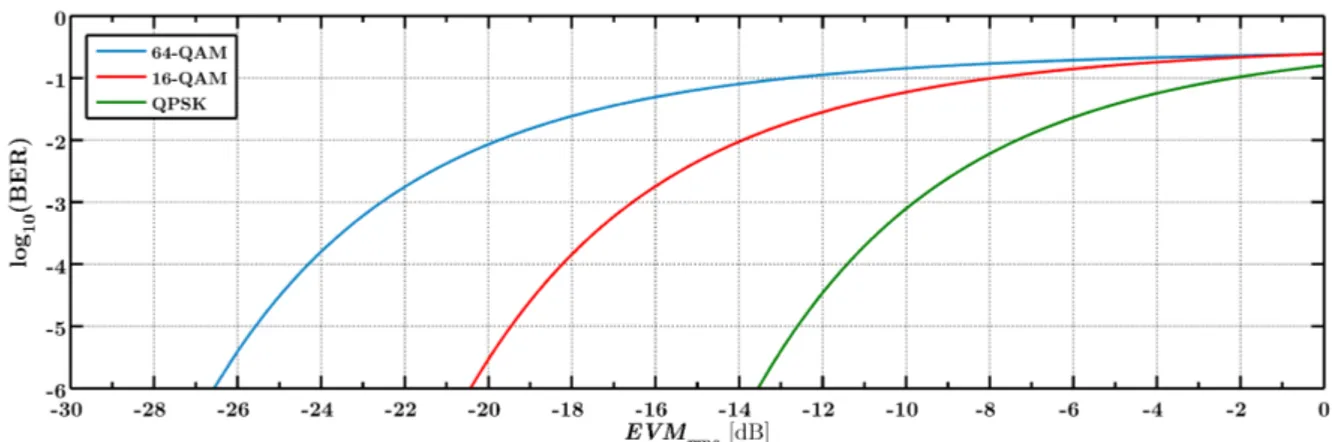
2.14 BER as a function of the EV Mrmsin dB. . . 27

3.1 Transfer function of the ideal filter. . . 30

3.2 Transfer function of n-order Super-Gaussian filter. . . 31

3.3 Transfer function of the integrator-and-dump filter. . . 32

3.4 Transfer function of the n-order Bessel filter. . . 33

3.5 Group delay of the n-order Bessel filter. . . 33

3.6 BER as a function of the required OSNR, using an ideal OF and integrator-and-dump EF, for the QPSK modulation format. . . 34

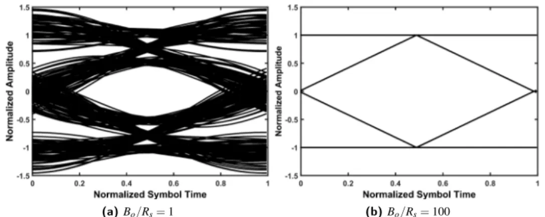
3.7 Eye diagrams of a QPSK signal with ideal filtering for (a) Bo/Rs= 1 and (b) Bo/Rs= 100 without ASE noise. . . 35

(16)

LIST OF FIGURES

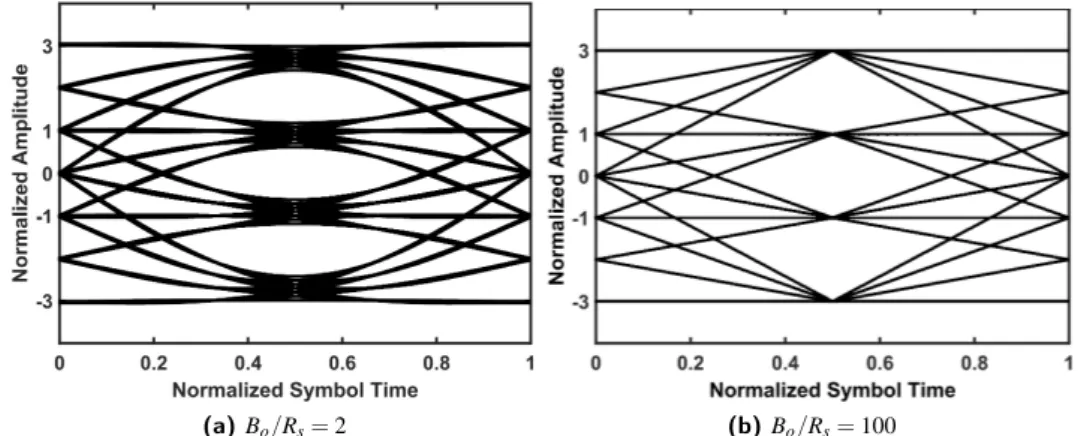
3.9 BER as a function of the required OSNR, using an ideal OF and an integrator EF, for the 16-QAM modulation format. . . 36 3.10 Eye diagrams of a 16-QAM signal with ideal filtering for (a) Bo/Rs= 2 and (b) Bo/Rs= 100

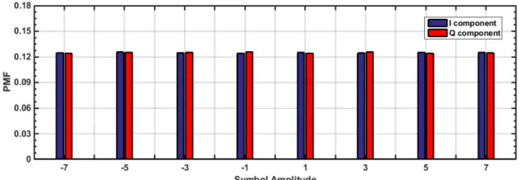
without ASE noise. . . 36 3.11 PMF of the symbols sequence amplitude for a 16-QAM signal. . . 37 3.12 BER as a function of the OSNR, using an ideal OF with Bo/Rs= 10 and an integrator EF, for

different 64-QAM symbols sequence lengths. . . 38 3.13 PMF of the symbols sequence amplitude for a 16-QAM signal with 218symbols. . . 39 3.14 BER as a function of the required OSNR, using an ideal OF and an integrator-and-dump EF, for

the 64-QAM modulation format. . . 39 3.15 Eye diagrams of a 64-QAM signal with ideal filtering for (a) Bo/Rs= 2 and (b) Bo/Rs= 100

without ASE noise. . . 39 3.16 BER as a function of the generated NMC with ideal filtering, obtained using the EVM method

and considering NMC= [1, 250]. . . 40 3.17 BER as a function of the OSNR by using the EVM method for the QPSK modulation format

and considering lower BERs. . . 41 3.18 BER as a function of the OSNR, for a QPSK ssignal with 50 Gbps using an ideal OF and an

integrator EF, estimated using the EVM, Equation (2.42) and the theoretical formula given by Equation (2.39). . . 42 3.19 BER as a function of the OSNR, for a 16-QAM signal with 50 Gbps using an ideal OF and an

integrator EF, estimated using the EVM, Equation (2.42) and the theoretical formula given by Equation (2.39). . . 42 3.20 BER as a function of the OSNR, for a 64-QAM signal with 50 Gbps using an ideal OF and an

integrator EF, estimated using the EVM, Equation (2.42) and the theoretical formula given by Equation (2.39). . . 43 3.21 Contour plots of the DEC (left side) and the EVM (right side) log₁₀(BER) estimates as a

func-tion of the normalized−3 dB bandwidths of the Gaussian OF and 5th-order Bessel EF, for the QPSK (a) NRZ, (b) RZ66, (c) RZ50 and (d) RZ33 receiver. . . 45 3.22 BER as a function of Bo/Rs for the Gaussian OF bandwidth and the NRZ, RZ66, RZ50 and

RZ33 pulse shapes, with OSNR=10.5 dB and having the 5th-order Bessel EF with a bandwidth of 1.1Rs. . . 46 3.23 Received eye diagrams of the QPSK modulation format with (a) NRZ, (b) RZ66, (c) RZ50

and (d) RZ33 pulse shapes, after Gaussian OF and 5th-order Bessel EF having the respective optimum−3 dB bandwidths. . . 47 3.24 Contour plots of the DEC (left side) and the EVM (right side) log₁₀(BER) estimates as a

func-tion of the normalized −3 dB bandwidths of the Gaussian OF and the Gaussian EF, for the QPSK (a) NRZ, (b) RZ66, (c) RZ50 and (d) RZ33 receiver. . . 48 3.25 Contour plots of the DEC (left side) and the EVM (right side) log₁₀(BER) estimates as a

func-tion of the−3 dB bandwidths for the 4th-order Super-Gaussian OF and the 5th-order Bessel EF, for the QPSK (a) NRZ, (b) RZ66, (c) RZ50 and (d)RZ33 receiver. . . 50

(17)

LIST OF FIGURES

3.26 Received eye diagrams of the QPSK modulation format with (a) NRZ, (b) RZ66, (c) RZ50 and (d) RZ33 pulse shapes, after Gaussian OF and 5th-order Bessel EF having the respective optimum−3 dB bandwidths. . . 51 3.27 Contour plots of the DEC (left side) and the EVM (right side) log₁₀(BER) estimates as a

func-tion of the−3 dB bandwidths for the 4th_{-order Super-Gaussian OF and the Gaussian EF, for the} QPSK (a) NRZ, (b) RZ66, (c) RZ50 and (d)RZ33 receiver. . . 52 3.28 Contour plots of the DEC (left side) and the EVM (right side) log₁₀(BER) estimates as a

func-tion of the normalized−3 dB bandwidths of the 4th-order Super-Gaussian OF and the 5th-order Bessel EF, with (a) NRZ, (b) RZ66, (c) RZ50 and (d)RZ33 pulse shapes for the 16-QAM receiver. 54 3.29 Received eye diagrams of the 16-QAM modulation format with (a) NRZ, (b) RZ66, (c) RZ50

and (d) RZ33 pulse shapes, after the fourth order Super-Gaussian OF and fifth order Bessel EF having the respective optimum−3 dB bandwidths. . . 56 4.1 Different types of crosstalk. . . 60 4.2 Optical network with in-band crosstalk coming from different sources. . . 61 4.3 Crosstalk simulation model for one sample function of in-band crosstalk and ASE noise in one

polarization. . . 63 4.4 (a) Time misalignment simulation, exemplified using a QPSK NRZ single interferer with a time

mismatch of Ts/2 in relation with the QPSK NRZ original signal, with Xc=0 dB and the (b) corresponding eye diagram. . . 63 4.5 Impact of (a) 0◦and (b) 45◦phase difference on the constellation of the selected signal. . . 64 4.6 PDFs of the QPSK NRZ received signal for an OSNR of 50 dB and a single QPSK NRZ

inter-ferer with the crosstalk levels of−25,−15 and −5 dB. . . 65 4.7 BER as a function of the OSNR for a QPSK NRZ interfering signal. The linear regression used

to estimate theδX T is also shown by the solid lines. . . 65 4.8 OSNR penalty as a function of the crosstalk level for a single interfering crosstalk signal

con-sidering the modulation formats QPSK, 16-QAM and 64-QAM with a symbol rate of 21.4 GBaud. 66 4.9 OSNR penalty as a function of the crosstalk level due to a single interfering signal with different

modulation formats but having the same pulse shape as the (a) QPSK NRZ, (b) QPSK RZ66 (c) QPSK RZ50 and (d) QPSK RZ33 selected optical signal. . . 68 4.10 Received constellations of the QPSK selected signal with a QPSK interfering signal having the

corresponding crosstalk level for 1 dB OSNR degradation for the (a) QPSK NRZ, (b) QPSK RZ66, (c) QPSK RZ50 and (c) QPSK RZ33 pulse shapes, respectively. . . 69 4.11 PDFs of the QPSK RZ33 selected signal having an OSNR of 11.2 dB, with QPSK RZ33,

16-QAM RZ33 and 64-16-QAM RZ33 interfering signals having a Xc,max of −13 dB, −14 dB and −15 dB, respectively. . . 70

4.12 Time misalignment influence due to a single interferer signal with different modulation formats and the same pulse shape as the (a) QPSK NRZ, (b) QPSK RZ66 (c) QPSK RZ50 and (d) QPSK RZ33 selected signal pulse shape. . . 72 4.13 Schematics of the interference of 16-QAM RZ33 pulse shape on the QPSK RZ33 selected

(18)

LIST OF FIGURES

4.14 OSNR penalty as a function of the normalized phase difference for a single interferer with the same or higher modulation format order than the (a) QPSK NRZ, (b) QPSK RZ66 (c) QPSK RZ50 and (d) QPSK RZ33 selected optical signals and having the same pulse shape as the original signal. . . 73 4.15 OSNR penalty as a function of the normalized phase difference between a 16-QAM RZ33

in-terfering signal and a QPSK RZ33 selected signal. . . 74 4.16 QPSK interfering signal constellation having a phase noise of 0 andπ/4 radians. . . 74

4.17 Eye diagrams of the QPSK interfering signal with a phase noise of (a)π/4 and (b) 0 radians. . . 75

4.18 OSNR penalty due to interfering signals with different duty-cycles but having the same mod-ulation format as the (a) QPSK NRZ, (b) QPSK RZ66 (c) QPSK RZ50 and (d) QPSK RZ33 selected optical signal. . . 76 4.19 Time misalignment influence on the OSNR penalty due to a single interferer with different

duty-cycles and having the same modulation format as the (a) QPSK NRZ, (b) QPSK RZ66 (c) QPSK RZ50 and (d) QPSK RZ33 selected optical signal. . . 77 4.20 Schematics of the interference of QPSK NRZ and RZ50 pulse shapes on the QPSK RZ50

se-lected signal, for a time mismatch of Ts/2. . . 78 4.21 OSNR penalty as a function of the normalized phase difference for a single interferer with

different duty-cycles and with the same modulation format order as the (a) QPSK NRZ, (b) QPSK RZ66 (c) QPSK RZ50 and (d) QPSK RZ33 selected optical signal. . . 79 4.22 OSNR penalty as a function of the crosstalk level due to interfering NRZ signals with different

binary rates and modulation formats than the QPSK NRZ selected optical signal, estimated by the (a) DEC method and the (b) EVM method. . . 80 4.23 OSNR penalty due to interfering NRZ signals with different binary rates and modulation formats

than the QPSK NRZ selected optical signal as a function of the (a) time misalignment and the (b) phase difference. . . 81 4.24 OSNR penalty as a function of the crosstalk level due to interfering signals with different

mod-ulation formats but having the same pulse shape as the (a) 16-QAM NRZ, (b) 16-QAM RZ66 (c) 16-QAM RZ50 and (d) 16-QAM RZ33 selected optical signal. . . 83 4.25 Received constellations of the 16-QAM RZ33 selected signal with a OSNR of 14.4 dB and a

16-QAM RZ33 interfering signal having the crosstalk level of−19 dB. . . 84 4.26 PDFs of the 16-QAM RZ33 selected signal with a OSNR of 14.4 dB and in the presence of a

QPSK RZ33, 16-QAM RZ33 and 64-QAM RZ33 interfering signals having the corresponding

(19)

List of Tables

2.1 QPSK mapping. . . 13 2.2 16-QAM mapping. . . 13 2.3 64-QAM mapping. . . 14 3.1 Simulation times of the sequences length optimization for the generation of 64-QAM random

symbols sequences. . . 38 3.2 Parameters for the QPSK system optimization. . . 44 3.3 Summary of the−3 dB bandwidths for the GB filters configuration, normalized to Rs, per pulse

shape, for the QPSK receiver, considering the DEC and EVM results. . . 46 3.4 Summary of the−3 dB bandwidths for the GG filters configuration, normalized to Rs, per pulse

shape, for the QPSK receiver, considering the DEC and EVM results. . . 49 3.5 Summary of the−3 dB bandwidths for the 4GB filters configuration, normalized to Rs, per

pulse shape, for the QPSK receiver, considering the DEC and EVM results. . . 51 3.6 Summary of the−3 dB bandwidths for the 4GG filters configuration, normalized to Rs, per

pulse shape, for the QPSK receiver, considering the DEC and EVM results. . . 53 3.7 Summary of the−3 dB bandwidths optimization, normalized to Rs, per pulse shape, for the

16-QAM receiver, considering the DEC and EVM results. . . 55 4.1 Required OSNR, without in-band crosstalk, for the QPSK receiver to reach a BER of 10−3per

pulse shape, using the indicated−3 dB bandwidths normalized to the symbol rate for the EF and the OF. . . 67 4.2 Simulation parameters used for the study of the time misalignment influence in the OSNR

degra-dation due to the crosstalk. . . 71 4.3 Simulation parameters to study the phase noise influence in the OSNR degradation due to the

crosstalk. . . 73 4.4 Required OSNR for the 16-QAM receiver for a BER of 10−3per pulse shape and per estimation

(20)

(21)

List of Acronyms

ASE Amplified Spontaneous Emission AWGN Additive White Gaussian Noise BER Bit Error Rate

DEC Direct Error Counting

DPSK Differential Phase-Shift Keying

DQPSK Differential Quadrature Phase-Shift Keying DSP Digital Signal Processing

ED Eye Diagram

EDFA Erbium-Doped Fiber Amplifier EF Electrical Filter

EVM Error Vector Magnitude FFT Fast Fourier Transform GF Galois Field

IP Internet Protocol

ISI Intersymbolic Interference LO Local Oscillator

M-PSK M-ary Phase-Shift Keying

M-QAM M-ary Quadrature Amplitude Modulation

MC Monte-Carlo OA Optical Amplifier OF Optical Filter OOK On-Off Keying

OPLL Optical Phase-Locked Loop OSA Optical Spectrum Analyzer OSNR Optical Signal-to-Noise Ratio PBS Polarization Beam Splitter PDF Probability Density Function

(22)

List of Acronyms

PDM Polarization Division Multiplexing PMF Probability Mass Function PRBS Pseudo-Random Bit Sequence PSD Power Spectral Density QF Quadrature Front-End

ROADM Reconfigurable Optical Add-Drop Multiplexer SE Spectral Efficiency

SNR Signal-to-Noise Ratio

(23)

List of Symbols

∆ f Frequency resolution δX T Penalty due to crosstalk

λ0 Selected signal wavelength

λX T Crosstalk signal wavelength F {} Fourier Transform

ν0 Optical carrier frequency

νLO Local oscillator optical frequency

ϕ(t) Signal phase ϕε Phase difference

B Bit rate

Be −3 dB bandwidth of the electrical filter Bo −3 dB bandwidth of the optical filter

Be,opt Optimized−3 dB bandwidth of the electrical filter Bo,opt Optimized−3 dB bandwidth of the optical filter BOSA Optical Spectrum Analyzer bandwidth

Bsim Simulation bandwidth E[.] Expected value

E0 Electrical field after optical filtering

ET(t) Transmitted electrical field Ex(t) Interfering signal electrical field E0,x(t) Electrical field in polarization x

E0,y(t) Electrical field in polarization y

ELO,x(t) Local oscillator electrical field in polarization x ELO,y(t) Local oscillator electrical field in polarization y h Planck constant

N0 ASE noise power spectrum density after optical filtering

(24)

List of Symbols

NI ASE noise power spectrum density of the in-phase component NQ ASE noise power spectrum density of the quadrature component Ns Number of symbols

Nx Total number of interfering signals NASE ASE noise power spectrum density NMC Number of MC sample functions P0 Average power of the selected signal

PLO Local oscillator power Rs Symbol Rate

T Overall duration of the simulated signal

Ta Sampling time

ti Time misalignment of the i-th interferer Ts Symbol time

Xc Crosstalk level

(25)

Chapter 1

Introduction

In the last years, the data traffic in the telecommunications networks had an exponential growth [1]. Figure 1.1 shows the evolution of the global Internet Protocol (IP) traffic since its beginning and the predicted growth until 2016. As it can be observed, the IP traffic in 2015 has increased about 10 orders of magnitude since 1980, and, in the next years, it is predicted that it continues to grow [1]. This increase of traffic demands the evolution of the telecommunications networks infrastructure in order to respond to the increasing communication need from users and also to technological advances. Optical technology has and will continue to enable telecommunication networks to support these traffic requirements [2].

Figure 1.1: Increase of the global IP traffic demands from 1985 to 2016 [1].

1.1 Road to 100 Gbps Optical Networks

The telecommunications networks are highly complex structures. So, in order to simplify the design, develop-ment and operation of those networks, it is common to use a layering approach [3]. Figure 1.2 exemplifies the

(26)

1.1. ROAD TO 100 GBPS OPTICAL NETWORKS Service Layer Transport Layer ROADM A ROADM B ROADM C ROADM D ROADM E IP a IP b IP c IP d

Figure 1.2: Layering approach for a telecommunication network [3].

layering concept for a telecommunication network. The upper layer is the service network layer and, nowadays, it is mainly formed by IP routers, which function is to gather and aggregate all information from the users. On the other hand, the transport network layer provides transmission paths for the service network layer, which are represented by colored dashed lines. In order to deliver high data capacity with lower signal loss, the transmis-sion medium that supports the transport network layer is the optical fiber. The network elements of the transport network layer represented in Figure 1.2 are Reconfigurable Optical Add-Drop Multiplexers (ROADMs).

The first optical networks served telephone services that required narrow bandwidth, a few kHz, but, as the communication services evolved, with the introduction of the Internet, the required bandwidth started to be more demanding. The IP has became the dominant traffic type in the service network layer, and the optical transport network has started to carry traffic from IP routers, MPLS (Multi-Protocol Label Switching) and Eth-ernet switches [1]. However, in the last decades, as shown in Figure 1.1, the IP traffic had a growth at a rate with a factor of ten [2], while the capacity of the optical transport networks has increased with a factor of four [1]. Figure 1.3 depicts the evolution of the optical transport network standard and the Ethernet port speed standard. Figure 1.3 shows that, in 2010, the deployment of OTU-4 standard allowed the optical channel capacity to reach the Ethernet port speed of 100 Gbps [1], [4].

The OTU-4 standard came from a long research work and several techniques to reach 100 Gbps were in-vestigated and tested. The elected approach was to adopt advanced detection schemes in order to increase the spectral efficiency (SE) per wavelength. Successful implementations were made by using optical differential detection, direct detection and coherent detection [4]. The latter detection technique was the telecom industry chosen for the OTU-4 standard [1]. The coherent detection allows the reception of high-order modulation sig-nals, which consequently, increases the SE of the optical signal transmission. In addition, this detection scheme combined with Polarization-Division Multiplexing (PDM) technique, doubles the SE of a given modulation format without requiring additional Optical Signal-to-Ratio (OSNR), by transmitting two modulated signals in the same optical carrier frequency, but with orthogonal polarizations [4]. By making use of wavelength

(27)

divi-CHAPTER 1. INTRODUCTION

Figure 1.3: Standards of the transport channel capacities and Ethernet port speeds [1].

sion multiplexing (WDM), optical systems with commercial capacities near 10 Tbps are commonly available nowadays [5].

1.2 Modulation Formats

The use of advanced modulation formats is also important to the increase of the optical networks capacity. Since 1985, until the deployment of the OTU-3 standard, On-Off Keying (OOK) was the elected modulation format for the optical transmission. On the receiver side, the detection of the incoming signal power was performed by a technique known as direct detection. The direct detection makes use of a photodiode to convert the optical signal power into an electrical current [6]. The use of optical amplification and WDM extended the use of direct detection and OOK in optical networks to the data rate of 10 Gbps until the end of 2000 [7].

With the deployment of the OTU-3 standard, the optical network reached the channel rate of 40 Gbps, and more modulation formats were used: the OOK 40 Gbps, and the differential modulation formats, such as Differential Phase-Shift Keying (DPSK) or the Differential Quadrature Phase-Shift Keying (DQPSK) [5], [8]. The detection of differential modulation formats is possible by including delay line interferometers and several photodiodes on the receiver, leading to the recovery of the phase information by estimating the phase difference between two consecutive symbols [6].

In 2010, the OTU-4 standard proposed a capacity of 100 Gbps per WDM channel in optical networks with the use of coherent receivers. Hence, the detection of Quadrature Phase-Shift Keying (QPSK) or M-ary Quadrature Amplitude Modulation (M-QAM) optical signals became possible, increasing the SE of the optical transmission. Despite the PDM-QPSK being the modulation format for the 100 Gbps optical networks, the coherent detection enables receiving other higher-order modulation formats. The detection of PDM-32-QAM [9] and PDM-64-PDM-32-QAM [10] signals at a bit rate of 100 Gbps has been also experimented [11].

(28)

1.3. IN-BAND CROSSTALK

are: 400 Gbps or 1 Tbps [1], [2], using higher-order QAM. Moreover, due to the higher OSNR required, and consequent shorter reach of the optical transmission, the 400 Gbps optical networks will require multi-carrier transmission, using superchannels [1], where the optical multi-carriers of the superchannel can be packed more tightly, without the use of guard bandwidth. However, these capacities are still in investigation and their future commercial deployment is not eminent [1]. There are several possibilities for the superchannel design at a data rate of 400 Gbps: using two carriers PDM-16-QAM superchannels, each one with a bit rate of 200 Gbps, or four carriers PDM-QPSK superchannels, each one with a bit rate of 100 Gbps [1]. The PDM-16-QAM superchannel occupies a total bandwidth of 82.9 GHz, and the PDM-QPSK superchannel has a bandwidth of 137.5 GHz. Thus, the total bandwidth of a superchannel, including the superchannels separation gap, is no longer multiple of the actual WDM networks, which have a fixed 50 GHz channel grid. Therefore, the data rate of 400 Gbps signals demands the adoption of a flexible grid, however it will increase the network management and digital signal processing complexity [1].

1.3 In-Band Crosstalk

In today 100 Gbps optical networks, a considerable amount of modulation formats and bit rates for the trans-mitted signals is possible and their coexistence can lead to more interference crosstalk scenarios than previous network environments.

The crosstalk is a physical impairment caused usually by the imperfect isolation of the optical components inside an optical node, i. e. ROADMs [12]. It originates signal power leakage inside each optical network node, and causes interference between signals that are propagating through the optical link.

The in-band crosstalk is the most detrimental type of crosstalk, since it occurs when the crosstalk and the se-lected signal have the same nominal wavelength [13]. Consequently, it is impossible to be removed by filtering and can become a serious source of system performance degradation [14], [15]. Moreover, the use of coherent detection receivers on the optical networks leads to a stronger interest in the in-band crosstalk study due to the coexistence of M-QAM modulation formats, OOK and differential modulation formats on the network [11]. Consequently, the interfering signals can have different modulation formats, leading to different impacts on the coherent receiver performance.

The in-band crosstalk and its impact on the network performance was extensively studied, for the OOK [14], DPSK [16] and DQPSK [17] modulation formats, and also for different modulation formats and bit rates than the selected signal [18], [19]. For example, in [19], it was found that the OOK signal is the most detrimental interfering signal in a DPSK 40 Gbps receiver.

However, few studies considering the in-band crosstalk impact on the performance of 100 Gbps coherent receivers can be found in the literature. The work [20] shows that, among the M-QAM modulation formats,

(29)

CHAPTER 1. INTRODUCTION

the one that presents greater tolerance to in-band crosstalk is the 4-QAM. In that work, it is considered that the interfering signals have the same modulation format and bit rate than the selected signal. In [21], the in-band crosstalk impact on a 112 Gbps PDM-QPSK receiver performance has been experimentally investigated con-sidering different modulation formats on the interferer. However, the results are not in agreement with [20], particularly, concerning the OSNR degradation of the coherent receiver due to higher crosstalk levels. In this dissertation, we intend to extend and clarify these studies and their conclusions, by studying the interference of signals with a wider variation of the signal parameters: different modulation formats with different orders, several bit rates and pulse shape duty-cycles. In addition, we will also assess the degradation of the 16-QAM coherent receiver performance due to the in-band crosstalk.

This dissertation will also investigate the accuracy of the Error Vector Magnitude (EVM) method in the presence of in-band crosstalk by comparing its estimates with the estimates obtained using Monte-Carlo (MC) simulation.

1.4 Dissertation Organization

The dissertation is organized as follows. The second chapter presents an introduction to coherent detection and its main theoretical concepts. The models for the electrical and optical components of the coherent detection receiver are provided and the methods for evaluating the bit error rate (BER) are described. Additionally, some MC simulation aspects are discussed.

In the third chapter, the filters used in this work are described, and the simulator validation is performed. The optimization of the filters bandwidths is also performed using the MC simulator and the EVM, for the 4-QAM and 16-QAM coherent receivers in presence of amplified spontaneous emission (ASE) noise. This optimization allows to choose the best optical and electrical filters configuration that minimizes the BER of the receiver in presence of ASE noise.

The fourth chapter introduces the crosstalk impairment theoretically and presents the model used in this work to address its impact. Then, the coherent receiver performance for the 4-QAM modulation format in the presence of in-band crosstalk is assessed, considering M-QAM interferers with different duty-cycles, different modulation formats and different bit rates. Additionally, the impact of the time misalignment and the phase difference between the selected and interfering signals is also studied and its influence on the coherent detection performance is discussed. Moreover, the influence of the in-band crosstalk on the 16-QAM coherent receiver performance is also investigated.

Finally, the fifth chapter summarizes the main conclusions obtained in this work and provides some ideas for possible future work.

(30)

1.5. MAIN ORIGINAL CONTRIBUTIONS

1.5 Main Original Contributions

In the analysis performed in this work, several original contributions were introduced relative to other studies in the field. In the following, the most important contributions of this work are presented:

• Comparison between the optimization of the−3 dB bandwidth for several non-ideal filters using the DEC and EVM methods, considering the QPSK and 16-QAM coherent receivers.

• Assessment of the impact of the in-band crosstalk on the coherent receiver performance, considering interferers with different modulation format orders and same bit rate as the selected signal.

• Assessment of the impact of the in-band crosstalk on the coherent receiver performance, considering interferers with different duty-cycles but with the same modulation format order as the selected signal. • Comparison between the assessment of the OSNR penalty at the M-QAM coherent receiver due to in-band

crosstalk using the DEC and EVM methods.

• Analysis of the influence of the time misalignment and phase difference between selected and interfering signals on the OSNR penalty variation due to in-band crosstalk.

(31)

Chapter 2

Optical Coherent Detection

2.1 Introduction

Nowadays, optical coherent detection is the chosen technology for the implementation of higher data rate net-works receivers since it enables the detection of higher SE optical signals. By adding the possibility of PDM signal detection, it is the elected detection technology for 100 Gbps or higher capacity networks [1].

In section 2.2, the coherent detection technique is presented and its advantages are described. Section 2.3 is dedicated to some relevant simulation aspects, such as the generation of the data sequences and its temporal and frequency representations. Also the MC simulation used in this work to study the coherent receiver is described. Then, in section 2.4, the signal modulation formats and duty-cycles considered in this dissertation are presented. The coherent receiver model is thoroughly described in section 2.5, with a particular emphasis on each com-ponent of the coherent receiver. Section 2.6 is dedicated to the analytic description of the coherent detected received signal corrupted by ASE noise. Lastly, in section 2.7, the simulation methods used in this work to assess the coherent receiver performance are described.

2.2 Coherent Detection

The optical coherent detection provides a great flexibility by enabling the reception of higher modulation formats, where the optical signal has its information encoded in the in-phase (I) and quadrature (Q) compo-nents [22], allowing to detect modulation formats with high SE such as M-ary Phase-Shift Keying (M-PSK) or

M-QAM signals. Alongside with the photodiodes and delay line interferometers (DLI)s, the coherent receiver

includes a local oscillator (LO), which signal is coupled with the incoming signal. And the demodulation of the received signal is made in the electrical domain, reducing the optical complexity due to the need of the

(32)

2.2. COHERENT DETECTION

DLIs to convert phase to intensity information [6], which is demanded in the demodulation of DPSK or DQPSK optical signals. However, the coherent detection drawback is in the synchronization between the LO signal and the optical signal. Three techniques have been designed to synchronize the LO with the received optical signal. Figure 2.1 illustrates those three techniques: (a) homodyne detection, (b) intradyne detection and (c) heterodyne detection.

Figure 2.1(a) shows the detected signal spectrum after homodyne detection, where the LO frequency (νLO) is the same as the incoming signal frequency (ν0). To synchronize the LO signal with the incoming signal, an

optical phase-locked loop (OPLL) is required. However, this component is sensible to propagation delay, which makes more difficult the receiver synchronization with the optical signal carrier frequency [6]. Another option is to assume that there is a frequency difference, typically of 100 kHz between both signals [23]. This technique is called intradyne detection and is depicted in Figure 2.1(b). This method uses a free-running local oscillator and has a similar detection bandwidth to the one of homodyne detection. To use a synchronized free-running LO without requiring the use of an OPLL, improved digital signal processing (DSP) technology must be used. Moreover, with the implementation of advanced DSP hardware in recent coherent systems, in substitution of the OPLL, the compensation of the chromatic dispersion and polarization mode dispersion is more efficient, since it is performed in the electrical domain [6].

In heterodyne detection, which is depicted in Figure 2.1(c), the LO frequency is different from the incoming signal carrier frequency. In this case, the optical signal is demodulated to an intermediate frequency fIF before the downconversion to baseband. The implementation of heterodyne detection is simpler than homodyne detec-tion, however the goal of accomplishing higher data rates with high SE, discards the heterodyne detection for optical reception due to the wider bandwidth required.

Coherent detection is usually combined with the PDM technique. This multiplexing technique doubles the SE by transmitting two modulated signals in the same optical carrier frequency, but with orthogonal polariza-tions. Hence, this multiplexing technique doubles the SE of any modulation format. For instance, if applied together with QPSK modulation, it quadruples the transmission capacity in comparison with the OOK for the same data rate [4].

ν0 0 ν0=νLO ν (a) Homodyne. ν ν0 0 ν0_{≈ ν}LO (b) Intradyne. ν0 0 νLO=ν0_{− f}if fif ν (c) Heterodyne.

(33)

CHAPTER 2. OPTICAL COHERENT DETECTION

The capability of receiving optical signals in which the information is encoded in amplitude, phase and polarization provides a higher spectral efficiency, and also enables the use of advanced DSP to compensate any linear impairment occurring during transmission. It remains to say that the coherent technique used in this work is the homodyne, since we will assume an ideal synchronization between the LO and the received signal.

2.3 System Simulation Aspects

In this section, the relevant aspects for the implementation of an optical communication system using computer simulation are briefly described. This description covers the generation of data sequences to represent an optical or an electrical signal and its time and frequency domain representations. Moreover, the MC simulation will also be explained.

2.3.1 Data Sequences

In computer simulations, a suitable choice of the symbols sequence is crucial for obtaining reliable results. Pseudo-random binary sequence (PRBS) are typically used to represent a binary data sequence [24]. By defi-nition, pseudo-random implies that the binary sequence is quasi-random and involves an algorithm to produce a periodic bit pattern with a specific length [25], in order to its autocorrelation function resembles the auto-correlation function of a random binary sequence [24]. Furthermore, in order to take into account the effect of intersymbol interference (ISI) accurately on the signal, the length of the bit pattern should be longer than the communication system memory [6]. However, as the length of the sequence increases, more computational effort is required to process all the symbols [6].

Since this work simulates M-QAM signals, symbols sequences are generated based on the same principle of the PRBS. In a M-ary communication system, the symbols sequences can be generated using Galois Fields (GF) arithmetic [24], which is based on the primitive polynomial of degree m defined by [6]

Pm(x) = xm+ am−1xm−1+ ... + a1x + a0 (2.1)

where aiis the coefficient in a finite field of q elements, Pm(x) is the minimal polynomial of a finite field GF(q) which can be implemented by a shift feedback register [24]. So, for the QPSK, the primitive polynomial of GF(22) is

(34)

2.3. SYSTEM SIMULATION ASPECTS

producing a sequence of 256 symbols. For 16-QAM sequences, the same g(x) is used to represent the I and Q components [24] with a 512 symbols length.

Since, the proper GF to generate 64-QAM symbols sequences was not a goal of this dissertation, the Matlab function rand is used for generate the symbols sequences for the 64-QAM modulation format. This function produces random numbers following a uniform distribution. However, the sequence length must be long enough to characterize the ISI with accuracy. The size of the sequence of the 64-QAM modulation format used in the simulation will be investigated in section 3.4.1.3.

T_a

Ts 2Ts (Ns_{− 1)}Ts NsTs₋Ta

Figure 2.2: Time vector representation.

In Matlab, the symbols sequences are described in the discrete time domain or in the frequency domain. The time vector is depicted in Figure 2.2. The number of positions of the time vector is NsNa, where Nsis the number of simulated symbols and Nais the number of samples per symbol. This will correspond to a continuous time, starting at the time instant t = 0 and finishing in T = NsTs− Ta, where Tsis the symbol time, Tacorresponds to the sampling time defined by Ta= Ts/Na, and T is the overall duration of the simulated signal [24].

Figure 2.3 shows the frequency vector, which has the same number of positions than the time vector, and where fais the sampling frequency defined as 1/Taand∆ f = 1/(NsTs) is the frequency resolution. The conver-sion of a signal in time domain to its frequency representation is computed using the Fast Fourier Transform, an algorithm that implements the Discrete Fourier Transform. Since this algorithm returns a shifted frequency vector, the Matlab function fftshift must be applied to rearrange the signal spectrum from [−fa

2,

fa

2− ∆ f ], where

the simulation bandwidth Bsimis as Bsim= fa− ∆ f .

∆f fa

2 − ∆f

−fa/2 −∆f

Figure 2.3: Frequency vector representation.

In the continuous time domain, the average power Pavgof a generic signal Es(t) is defined by [26]

Pavg= 1 T ∫ _T 0 |Es (t)|2dt (2.3)

(35)

In computational simulations, Equation (2.3) can be estimated using the Matlab function trapz which imple-ments the trapezoidal method.

The power spectrum density (PSD) of the simulated signal is estimated using the definition of periodogram defined by [26] GE( f ) = 1 T|Es( f )| 2 _(2.4)

2.3.2 Monte-Carlo Simulation

The MC method is a well known algorithm for statistical simulations in various scientific areas, where there is the need to describe a stochastic process. This method implements a sequence of Bernoulli trials [24], by generating random sequences of numbers based on a certain probabilistic distribution. These random sequences of numbers represent sample functions of the stochastic process intended to be studied.

Start Ideal transmiter iteration=0 Addition of a statistical sample function Save reference signal Receiver Obtain delay and the optimum time sampling Synchronism and signal sampling Comparison with reference signal Stopping criteria is achieved ? Performance estimation End no sample0 sample0 yes no yes sample0

(36)

2.4. TRANSMITTER DESCRIPTION

The MC simulation will be described using the flow-chart depicted in Figure 2.4. In the first iteration of the MC simulation, an optical signal with a specific modulation format, such as M-QAM or M-PSK is generated using an ideal transmitter, and it is propagated along the receiver without the addition of any statistical sample function. This first iteration is called the sample0. The detection of this sample will provide a reference signal to

the receiver, in order to know which symbols were transmitted. The reference signal is also used to measure the propagation delay of the communication system, in order to assure the synchronization between received and transmitted signals. Then, on the following iterations, random sample functions of the stochastic process are generated and added to the signal, modifying the optical signal at the receiver input. At the end of each iteration, the received symbols are compared with the corresponding symbols of the reference signal, and depending of the assessment method used, the performance of the receiver is estimated. As a stopping criteria, the simulation ends when a pre-defined total number of symbols errors is achieved or a total of samples functions is generated [24]. The ASE noise will be the stochastic process impairing the coherent receiver performance in chapter 3, and in chapter 4, the stochastic processes will be the ASE noise and the in-band crosstalk.

2.4 Transmitter Description

In optical coherent communication systems, the generation of the optical signal is usually accomplished using a laser followed by an IQ modulator [27]. For the sake of simplicity, we will assume an ideal transmitter throughout this work. The optical signal is parametrized by its modulation format, symbol duration, duty-cycle, pulse shape and average power.

2.4.1 Modulation Formats and Constellations

In this subsection, the generation of optical signals with M-ary QAM modulation format is explained. The structure of a M-ary transmitter is shown in Figure 2.5, where the symbols sequence is fed into the mapping block. The main function of this block is to assign at its outputs the amplitude levels corresponding to the

Constelation Mapping 90◦ + ET[k] I[k] Q[k] symbol[k]

(37)

(a) 4-QAM/QPSK. (b) Square 16-QAM. (c) Square 64-QAM.

Figure 2.6: Ideal constellations for (a) QPSK, (b) 16-QAM and (c) 64-QAM mappings signals.

in-phase I[k] and quadrature Q[k] components [26] accordingly to the sequence of symbols at its input,

I[k] =±1,±3,....,±(√M− 1) Q[k] =±1,±3,....,±(√M− 1)

(2.5)

The signal in the I branch is added to the 90◦shifted signal in the Q branch resulting in the complex symbol sequence ET[k] = I[k] + jQ[k].

Tables 2.1, 2.2 and 2.3 present the mapping used between bits and symbols at the output of the IQ mapper and Figure 2.6 shows the constellations for the (a) 4-QAM, (b) 16-QAM and (c) 64-QAM modulation formats. Figure 2.7 shows the power spectral density (PSD) of the M-QAM modulated signals having an average power of 1 mW and a 50 Gbps bit rate per polarization, which corresponds to a 100 Gbps signal when using PDM, for (a) QPSK, (b) 16-QAM and (c) 64-QAM signals. For the QPSK modulation format, the bandwidth

Symbol bits ET[k] 1 00 −1 − j 2 01 −1 + j 3 11 1− j 4 10 1 + j Table 2.1: QPSK mapping.

Symbol bits ET[k] Symbol bits ET[k]

1 0000 −3 − 3 j 9 1000 3− 3 j 2 0001 −3 − j 10 1001 3− j 3 0010 −3 + 3 j 11 1010 3 + 3 j 4 0011 −3 + j 12 1011 3 + j 5 0100 −1 − 3 j 13 1100 1− 3 j 6 0101 −1 − j 14 1101 1− j 7 0110 −1 + 3 j 15 1110 1 + 3 j 8 0111 −1 + j 16 1111 1 + j

(38)

2.4. TRANSMITTER DESCRIPTION

Symbol bits ET[k] Symbol bits ET[k] Symbol bits ET[k] Symbol bits ET[k]

1 000000 −7 − 7 j 17 010000 − j − 7 j 33 100000 7− 7 j 49 110000 1− 7 j 2 000001 −7 − 5 j 18 010001 − j − 5 j 34 100001 7− 5 j 50 110001 1− 5 j 3 000010 −7 − j 19 010010 − j − j 35 100010 7− j 51 110010 1− j 4 000011 −7 − 3 j 20 010011 − j − 3 j 36 100011 7− 3 j 52 110011 1− 3 j 5 000100 −7 + 7 j 21 010100 − j + 7 j 37 100100 7 + 7 j 53 100100 1 + 7 j 6 000101 −7 + 5 j 22 010101 − j + 5 j 38 100101 7 + 5 j 54 100101 1 + 5 j 7 000110 −7 + j 23 010110 − j + j 39 100110 7 + j 55 100110 1 + j 8 000111 −7 + 3 j 24 010111 − j + 3 j 40 100111 7 + 3 j 56 100111 1 + 3 j 9 001000 −5 − 7 j 25 011000 −3 − 7 j 41 101000 5− 7 j 57 111000 3− 7 j 10 001001 −5 − 5 j 26 011001 −3 − 5 j 42 101001 5− 5 j 58 111001 3− 5 j 11 001010 −5 − j 27 011010 −3 − j 43 101010 5− j 59 111010 3− j 12 001011 −5 − 3 j 28 011011 −3 − 3 j 44 101011 5− 3 j 60 111011 3− 3 j 13 001100 −5 + 7 j 29 011100 −3 + 7 j 45 101100 5 + 7 j 61 111100 3 + 7 j 14 001101 −5 + 5 j 30 011101 −3 + 5 j 46 101101 5 + 5 j 62 111101 3 + 5 j 15 001110 −5 + j 31 011110 −3 + j 47 101110 5 + j 63 111110 3 + j 16 001111 −5 + 3 j 32 011111 −3 + 3 j 48 101111 5 + 3 j 64 111111 3 + 3 j

Table 2.3: 64-QAM mapping.

of the main lobe is 50 GHz (Figure 2.7(a)) and the SE is 2 bits/s/Hz; for the 16-QAM (Figure 2.7(b)), the SE is 4 bits/s/Hz with 25 GHz of main lobe bandwidth, and for the 64-QAM (Figure 2.7(c)) the SE is 6 bits/s/Hz with a main lobe bandwidth 16.67 GHz.

(a) QPSK. (b) 16-QAM. (c) 64-QAM.

Figure 2.7: PSD of the simulated (a) 4-QAM, (b) 16-QAM and (c) 64-QAM signals.

2.4.2 Duty-Cycle

The shape of the optical pulse can affect significantly the performance of the optical fiber communication system [6]. Assuming ideal synchronization at the receiver, we will study four pulse shapes - the return-to-zero (RZ) with duty- cycles of 66, 50 and 33%, and the non return-to-zero (NRZ) with a 100% duty-cycle.

The rectangular NRZ pulse shape is characterized by having the optical power of each symbol constant throughout the duration of the symbol time. This format has the advantage of having a smaller bandwidth and therefore is commonly used in systems where bandwidth requirements are stringent, for instance in WDM channels [27]. Its main disadvantage is that is highly vulnerable to dispersion and nonlinear effects caused by

(39)

fiber transmission [27]. The RZ format is characterized for having the null optical power before the symbol time is over. There are several variants of RZ pulse, depending on the Tp/Tsratio, referred as the duty-cycle, where Tpis the pulse duration and Tp< Ts. The duty-cycle can vary depending on the transmission goals because it affects directly the signal bandwidth. For instance, for a duty-cycle of 50%, the corresponding bandwidth will be twice the NRZ signal bandwidth. Therefore, this pulse shape, when applied in WDM systems, reduces the SE of the transmission, since it demands a larger separation between two consecutive WDM signals [28].

Figure 2.8 shows a (a) rectangular NRZ signal and a (b) rectangular RZ signal with 50% duty-cycle, as a function of the normalized symbol time, and the bandwidth of the NRZ and RZ50 are depicted in (c) and (d), respectively.

(a) NRZ signal (b) RZ signal

(c) NRZ PSD (d) RZ 50% PSD

Figure 2.8: Temporal representation of a (a) NRZ and (b) RZ with 50% duty-cycle pulse shapes and its respective PSDs, (c) and (d).

(40)

2.5. COHERENT RECEIVER MODEL

2.5 Coherent Receiver Model

In this section, the model used in this work for the coherent receiver with PDM is described. Figure 2.9 depicts the block diagram of the coherent receiver. The lowpass equivalent of the PDM signal, EPDM(t), at the coherent receiver input is defined as

EPDM(t) = ET ,x(t) ˆx + ET ,y(t) ˆy (2.6) where ET ,x(t) and ET ,y(t) are the transmitted optical signals in the orthogonal polarizations, which directions are defined by the unit vectors ˆx and ˆy. N(t) represents the lowpass equivalent of the ASE noise in both polarizations

and it will be described in the next subsection.

The model in Figure 2.9 consists of an optical filter (whose characterization will be made in chapter 3), two polarization beam splitters (PBSs) and two Quadrature Front-ends (QFs). The optical amplifier is considered in Figure 2.9, as the addition of the noise to the signal. One PBS is used to split the PDM incoming signal having ASE noise in both polarizations E0,x(t) + N0,x(t) and E0,y(t) + N0,y(t), which will be detected in their respective

QF. The PBS is also applied to the LO signal, in order to separate its two polarizations: ELO,xand ELO,y. The goal of the QF is to detect individually the I and Q components of the input signal. At the output of the QF, the I and Q components, in each polarization, are added to form the currents Ix(t) and Iy(t).

The following subsections describe each component of the coherent receiver with more detail.

Optical Filter + PBS PBS ∼ Quadrature Front-end Quadrature Front-end + + E0(t) + N0(t) II,x(t) IQ,x(t) Ix(t) II,y(t) IQ,y(t) Iy(t) E0,x(t) + N0,x(t) E0,y(t) + N0,y(t) ELO,x ELO,y EP DM(t) LO N(t)

Figure 2.9: Schematic block diagram of a PDM coherent receiver with an optical quadrature frontend.

2.5.1 Optical Amplification

On an optical network, the fiber transmission media causes signal attenuation, as well as several network ponents, like multiplexers/demultiplexers, couplers and ROADMs. So, signal amplification is required to com-pensate those losses [7], [29].

There are three main types of optical amplifiers (OA): Erbium-Doped Fiber Amplifier (EDFA), Semicon-ductor Optical Amplifiers and Raman amplifiers. The most commonly used amplifier is the EDFA, since it can

(41)

achieve a gain of about 30 dB and operates in the C band (1530-1565 nm), the wavelength band normally used for optical communications [29]. However, the amplification also adds ASE noise to the signal [7]. In lumped amplification, the ASE noise is accumulated along a chain of cascaded OAs and the resulting ASE noise power of all the amplifiers can be measured at the end of the fiber link using the OSNR, which is defined by

OSNR = Pin

PASE

(2.7)

where Pinis the accumulated power of the signal summed over the two states of polarization [30] and PASE is the average ASE noise power, which is defined, for both noise polarizations, by

PASE= 2NASEBOSA (2.8)

where BOSAis the Optical Spectrum Analyzer (OSA) bandwidth with the typical value of 12.5 GHz [25]. The OSA is a measurement instrument that is used to evaluate the OSNR at a determined wavelength and BOSA is related to the simulation bandwidth Bsimby [25]

BOSA=

BsimPASE 2Pn

(2.9)

where Pnis the ASE noise power used in the simulation. The ASE noise PSD, of one polarization, is given by

NASE= nsphν0.(g− 1) (2.10)

where nspis the spontaneous emission noise factor, h is the Planck constant1, and g is the power gain.

The ASE noise, in each polarization, NASE(t), is considered to be an Additive White Gaussian Noise (AWGN), which can be expressed by its lowpass equivalent signal

NASE,m(t) = 1

√

2(NI(t) + jNQ(t)) , m = x or y (2.11) where NI(t) and NQ(t) are respectively, the I and Q components of the ASE noise field. Therefore

N(t) = NASE,x(t) ˆx + NASE,y(t) ˆy (2.12)

The ASE noise has a zero mean and its variance is defined by

E[NASE(t)NASE∗ (t′)] = N0δ(t−t′) (2.13)

(42)

where E[.] is the expected value andδ(t) represents the Dirac delta function. The property

E[NASE(t).NASE(t′)] = 0 (2.14)

is also useful to the derivations presented in this work.

2.5.2 Local Oscillator

The LO is an essential component of the coherent receiver, which signal is required to be mixed with the incoming signal, allowing the recover of the information encoded in the I and Q components of the received optical signal [23]. In order to maximize the coherent receiver performance, the LO frequency must be as close as possible to the optical carrier frequency [23]. Furthermore, if the LO is tunable, it can be equivalent to an ultranarrow WDM optical filter at the front of the coherent receiver [31].

In this work, the LO is considered synchronized with the optical carrier frequency and the intensity noise is neglected. The electrical field of LO signal is defined as:

ELO(t) = √

PLOejϕLO(t) (2.15)

whereϕLO(t) is the phase of the LO laser signal and PLO is the LO optical power, which is typically 30 dB higher than the received signal optical power [23].

2.5.3 Quadrature Front-End

Each OFQ, in Figure 2.9 is formed by a 2 x 4 90◦Hybrid and two balanced photodetectors followed by a post-detection filter, for reducing the noise and ISI after photopost-detection [6]. In the following, the model used in this work for these components will be described.

2.5.3.1 Hybrid

There are various possibilities of implementing a hybrid as illustrated in Figure 2.10 [6]. The most common and commercially available configuration is the one composed by four 3 dB couplers, (Figure 2.10(a)). The 90° phase shift in the lower branch guarantees orthogonality between the two branches, and allows the detection of the I and Q signal components.

Another alternative to implement this hybrid is the 4 x 4 Multi-Mode interference (MMI) coupler, which configuration is depicted in Figure 2.10(b). This component is constructed by dimensioning the waveguides that constitute the device in order to provide the phase relations required by a 90°hybrid. Furthermore, the balanced

(43)

CHAPTER 2. OPTICAL COHERENT DETECTION 3 dB 3 dB 90◦ 3 dB 3 dB E0 ELO E2 E4 E1 E3

(a) Hybrid with 3 dB coupler.

4x4 MMI

Eout,1 Eout,4 Eout,2 Eout,3 E0 ELO (b) MMI 4x4.

3 dB

PBS

E0 ELO E_out,1 Eout,2 Eout,3 Eout,4 (c) Integrated device.

Figure 2.10: Different configurations of a hybrid.

photodetectors can be integrated, which means that the QF can be fully implemented ona chip, using a MMI coupler [6]. Another interesting characteristic of MMI couplers is their wide bandwidth, which makes them a suitable component for WDM, however this device is not yet commercially available.

The third option is an integrated device of discrete components, composed by two PBS and a 3 dB coupler, as shown in Figure 2.10(c). However, this device requires specific polarizations states for each input signal [6]. In this work, the 2 x 4 90° hybrid depicted in Figure 2.10(a) will be modeled, since it is the most commonly used in optical communications.

The model of the hybrid used in this dissertation is described in the following. We start by introducing the 3 dB coupler. This component is a special case of a directional coupler, which is a passive device constructed from two coupled transmission lines, set closely together such that the energy passing through one arm of the coupler is coupled to the field in the other arm. Structurally, the directional coupler has two inputs and two outputs, intermediated by the coupling region with length Lc[28], as depicted in Figure 2.11. Equation (2.16) describes the output electrical fields of the directional coupler [27],

  Eo,1(t) Eo,2(t)   =   √ρ j√1−ρ j√1−ρ √ρ     Ei,1(t) Ei,2(t)   (2.16)

(44)

whereρis the power coupling coefficient. To get a 3 dB coupler,ρ must equal 0.5, so, the two electric fields at the output of the 3 dB coupler are given by:

Eo,1(t) = 1 √ 2(Ei,1(t) + jEi,2(t)) Eo,2(t) = 1 √ 2( jEi,1(t) + Ei,2(t)) (2.17)

An important feature of the 3 dB coupler is to provide two coupled outputs with an 180° shift phase differ-ence between them, and is often known as an 180° hybrid. The 3 dB coupler is a very versatile device since it can be applied to different functions. If only one input is fed, the result is a power divider. If the two inputs are active and only one output inactive, we have a power combiner. A power divider is obtained by making

Ei,2(t) = 0 in Equation (2.17), and the output electric fields become:

Eo,1(t) = E_√i,1(t) 2 Eo,2(t) = j E_√i,1(t) 2 (2.18)

A similar result is obtained by making Ei,2(t) active and Ei,1(t) = 0. By considering Figure 2.10(a) and taking the proper input electrical fields definitions, the transfer function of the 2 x 4 90° hybrid is [6]:

        E1(t) E2(t) E3(t) E4(t)         =1 2         1 −1 j j j −1 −1 j           Es(t) ELO(t)   (2.19)

2.5.3.2 Polarization Beam Splitter

The PBS consists of a fiber-based Mach-Zehnder interferometer (MZI) [32], consisting of two 3 dB couplers with two delay lines as shown in Figure 2.12 [25].

This device is used to separate the input optical signal into horizontal and vertical polarization components. In ideal conditions, the input PDM signal power is equally split between the two outputs of the PBS [25], i.e.

Pp= Pin/2, where Pp is the average signal power of each PBS output. Since the signal power is halved, the respective PASE is proportionally reduced, which means PASE,p= PASE/2 = NASEBOSA. Therefore, the OSNR of each polarization (OSNRp) is given by [30]

OSNRp= Pp NASEBOSA = Pin 2NASEBOSA (2.20)

(45)

where OSNRp defines the OSNR in each polarization, which means that the OSNR after an ideal PBS for a PDM ideal optical signal is the same as if the optical signal has been transmitted in a single polarization.

Figure 2.12: Mach-Zehnder interferometer

2.5.3.3 Photodetector

In order to recover all the information from an optical signal, an optical-electrical conversion has to be performed using a photodetector. These devices are made of semiconductors materials to respond to the requirements demanded by a lightwave system: high sensitivity, low noise, fast response, high reliability and a size compatible with the fiber core [7]. The operation of a photodetector can be described by its responsivity defined by [7]:

R_λ= Ip(t)

Pin(t)

[A/W ] (2.21)

where Ip(t) is the current produced by the incident optical power Pin(t) on the photodetector. In this work, for simplification, a unit responsivity, i.e. R_λ = 1 A/W will be assumed. Hence Pin(t) =|Ein(t)|2, where Ein(t) is the electrical field incident on the photodetector.

2.5.3.4 Post-Detection Electrical Filter

All optical receivers have a low-pass filter for reducing the noise and ISI after photodetection [6]. This post-detection filter also models the frequency limitations of the photodetector.

The filter design aims maximizing the electrical Signal-to-Noise (SNR) at the decision circuit input, so the shape of the filter must be closely, or ideally, the same as the incoming signal. A filter with this property is called a matched filter [33]. In fact, one of the most important objective in the design of filters is that, its shape must be as close to the ideal shape as possible. The 4th-order Super Gaussian or the 5th-order Bessel filter are some examples of filters typically used [34], [35].

2.6 Detected Signal Statistics

This section describes the theory and the mathematical analysis behind the detection of the electrical I and Q components of the optical signal in one polarization direction.

(46)

2.6. DETECTED SIGNAL STATISTICS . . E0(t) + N0(t) . ELO . 90◦ . 2 x 4 90◦Hybrid . E1(t) . E3(t) . E2(t) . E4(t) . I1(t) . I3(t) . I2(t) . I4(t) . II(t) . IQ(t) . h(t) . h(t) . + . − . + . −

Figure 2.13: Setup of a typical QF based on the configuration presented in Figure 2.9.

fields at the four photodetectors inputs are described by:

E1(t) = 1 2[(E0(t) + N0(t))− ELO(t)] E2(t) = j 2[(E0(t) + N0(t)) + ELO(t)] E3(t) = 1 2[ j(E0(t) + N0(t))− ELO(t)] E4(t) = 1 2[−(E0(t) + N0(t)) + jELO(t)] (2.22)

After square-law photodetection, the output photocurrent in each photodetector is written, respectively, as:

I1(t) = 1 4|(E0(t) + N0(t)) + ELO(t)| 2 I2(t) = 1 4|(E0(t) + N0(t)) + jELO(t)| 2 I3(t) = 1 4|(E0(t) + N0(t))− ELO(t)| 2 I4(t) = 1 4|(E0(t) + N0(t))− jELO(t)| 2 (2.23)

By developing the absolute square of complex number in each term, we have:

I1(t) = 1 4 [[ |(E0|2+|N0|2+ 2ℜ{E0N0∗} ] +|ELO|2− 2ℜ{E0ELO∗ + N0ELO∗ } ] I2(t) = 1 4 [[ |(E0|2+|N0|2+ 2ℜ{E0N0∗} ] +|ELO|2+ 2ℜ{E0ELO∗ + N0ELO∗ } ] I3(t) = 1 4 [[ |(E0|2+|N0|2+ 2ℜ{E0N0∗} ] +|ELO|2− 2ℑ{E0ELO∗ + N0ELO∗ } ] I4(t) = 1 4 [[ |(E0|2+|N0|2+ 2ℜ{E0N0∗} ] +|ELO|2+ 2ℑ{E0ELO∗ + N0ELO∗ } ] (2.24)

whereℜ{Z} and ℑ{Z} stands for, respectively, the real part and the imaginary part of a complex number Z, with the complex conjugate represented by Z∗. Next, the I and Q components are defined as: II(t) = I2(t)−I1(t)

Impact of in-band crosstalk on the performance of optical coherent detection communication systems

D

EPARTMENT OF INFORMATION SCIENCE AND TECHNOLOGY