6th World Congresses of Structural and Multidisciplinary Optimization Rio de Janeiro, 30 May - 03 June 2005, Brazil
CORE AND PATCH POSITION OPTIMIZATIONS FOR VIBRATION CONTROL OF
PIEZOLAMINATED STRUCTURES
José M. Simões Moita
1, Victor M. Franco Correia
2, Cristóvão M. Mota Soares
3, Carlos A. Mota Soares
3 1Universidade do Algarve, Escola Superior de Tecnologia, Faro, Portugal. E-mail: [email protected]
2
ENIDH–Escola Náutica Infante D. Henrique, Paço de Arcos, Portugal.
3
IDMEC/IST–Instituto Superior Técnico, Lisboa, Portugal. 1. Abstract
This paper deals with a finite element formulation based on the classical laminated plate theory, for active control of thin plate laminated structures with integrated piezoelectric layers, acting as sensors and actuators. The control is initialized through a previous optimization of the core of the laminated structure, in order to minimize the vibration amplitude. Also the optimization of the patches position is performed to maximize the piezoelectric actuator efficiency. The simulating annealing method is used for these purposes. The finite element model is a single layer triangular nonconforming plate/shell element with 18 degrees of freedom for the generalized displacements, and one electrical potential degree of freedom for each piezoelectric element layer, which can be surface bonded or imbedded on the laminate.
To achieve a mechanism of active control of the structure dynamic response, a feedback control algorithm is used, coupling the sensor and active piezoelectric layers. To calculate the dynamic response of the laminated structures the Newmark method is considered. The model is applied in the solution of an illustrative case and the results are presented and discussed.
2. Keywords: Active Control, Sensors and Actuators, Adaptive Laminated Structures, Structural Optimization. 3. Introduction
Advanced reinforced composite structures incorporating piezoelectric sensors and actuators are increasingly becoming important due to the development of adaptive structures. These structures offer potential benefits in a wide range of engineering applications such as vibration and noise suppression, shape control and precision positioning.
In the analysis of adaptive structures integrating piezoelectric material, one of the pioneering works is due to Allik and Hughes [1] who developed a solid finite element for vibration analysis. Vibration control of composite beams with embedded or surface bonded piezoelectric material had been studied by Crawley and de Luis [2]. Tzou and Tseng [3] presented a finite element formulation for plates and shells containing integrated distributed piezoelectric sensors and actuators applied to control advanced structures. Chen et al. [4] developed a finite element based on the first order displacement field for dynamic analysis of plates. Active control is obtained through actuators potential, which is given by an amplified signal of the sensors potential.
Using a higher order shear deformation theory Samanta et al. [5] developed an eight-nodded finite element for the active vibration control of laminated plates with piezoelectric layers acting as distributed sensors and actuators. The active control capability is studied using a simple algorithm with negative velocity feedback. Lam et al. [6] and Moita et al. [7] developed finite element models based on the classical laminated theory for the active control of composite plates containing piezoelectric sensors and actuators using the Newmark method [8] to calculate the dynamic response of laminated structures. Reviews of the modelling and the design of composite structures with adaptive capabilities are given in Franco Correia et al. [9] and Benjeddou [10].
Batra and Liang [11] used a three-dimensional linear theory of elasticity to find the optimal location of an actuator on a simple-supported rectangular laminated plate with embedded PZT layers. The optimal design is obtained by fixing the applied voltage and the size of the actuator and moving it around in order to find the maximum out-of-plane displacement. Liang et al. [12] proposed a model for the optimization of the induced-strain actuator location and configuration for active vibration control. Correia et al. [13] presented refined finite element models based on higher order displacement fields applied to the optimal design of laminated composite plates with embedded or surface bonded piezoelectric actuators and sensors.
Most of past work in the area of adaptive structures has focused on the analysis of structures with sensors and actuators, and the corresponding associate control system. Very few works have focused on the development of methodologies for the optimization of laminated structures incorporating sensors and actuators, to enhance their performance. A review of the current work in design methodologies and applications of formal optimization methodologies for adaptive structures has been carried out by Padula [14] and Frecker [15].
The finite element used in the present work is a flat three-nodded triangular element with 18 mechanical degrees of freedom and one electric degree of freedom per piezoelectric layer of the finite element and is based on the classical laminated plate theory. An integrated control is considered in order to achieve an active damping mechanism, with the amplified electrical potential of the sensors being used as electric potential input to the actuators through a negative velocity feedback control. The governing equations are solved by the Newmark method, which is a direct method for time integration. Priory to the dynamic control, to minimize the (forced) vibration amplitude through active damping, an optimal lamination sequence of the structure core, as well as an optimal placement of piezoelectric actuators patches are carried out using a structural optimization methodology based on simulated annealing algorithm [16].
4. Displacement and strain fields.
The assumed displacement field is that of the classical laminated plate theory. The displacement components referenced to the local axis (x,y,z) of the laminate are:
(
x,y,z)
u( )
x,y z( )
x,yu = 0 − θy
v
(
x,y,z)
=v0( )
x,y+zθx( )
x,y (1)(
x,y,z)
w( )
x,yw = 0
where
u
0,
v
0,
w
0 are displacements of a generic point in the middle plane of the laminate referred to the local axes - x,y,z directions,θ
x
,
θ
y
are the rotations of the normal to the middle plane, about the x and y axis, respectively.The strains components associated with the displacements in equation (1) are
x z x u xx y 0 ∂ θ ∂ − ∂ ∂ = ε y z y v = 0 x yy ∂ θ ∂ + ∂ ∂ ε (2) ∂ ∂ ∂ ∂ − ∂ ∂ ∂ ∂ = γ x θ + y θ z x v + y u xy 0 0
+
y x5. Piezoelectric Laminates. Constitutive Equations.
Assuming that a piezoelectric composite plate consists of several layers, including the piezoelectric layers, the constitutive equation for an orthotropic layer of the laminate substrate, is
ε
σ
=
Q
(3)and the constitutive equations of a deformable piezoelectric material, coupling the elastic and the electric fields are given by, Tiersten [17]
E
e
Q
ε
σ
=
−
(4)E
p
e
D
=
Tε
+
(5)where σ=
[
σxxσyyσxy]
Tis the elastic stress vector and ε=[
εxxεyyγxy]
T the elastic strain vector, Q the elastic constitutive matrix,e
the piezoelectric stress coefficients matrix, E=[
Ex Ey Ez]
Tthe electric field vector,[
]
T z y xD D D D= the electric
displacement vector and
p
the dielectric matrix, in the element local system (x,y,z) of the laminate. Qij,e
ij,p
ij are functions of ply angle α for the kth layer, and are given explicitly in Reddy [18].The electric field vector is the negative gradient of the electric potential
φ
, which is assumed to be applied in the thicknesst
k
direction, where it can vary linearly, i.e.φ −∇ = E (6)
{
}
T z E 0 0 = E(7) where k z /t E =−φ (8)
Thus, we can define the strain vector for electro elasticity as follows
− = E εˆ ε (9)
where the mechanical strain vector can be represented as follows: b z m
=ε ε
ε + (10)
Thus, the constitutive equations (4) and (5) can be written in the form:
ε ε σ ˆ ˆ E p -e e Q D σ ˆ T =C − = = (11)
6. Finite element formulation.
The flat triangular finite element model has three nodes and six degrees of freedom per node, the displacements
i i
i 0 0
0 , v , w
u and
rotations θxi,θyi ,θzi. The introduction of fictitious stiffness coefficients Kθz, corresponding to rotationsθz, to eliminate the
problem of a singular stiffness matrix, for which the elements are coplanar or near coplanar, is required. The element local displacements, slopes and rotations are expressed in terms of nodal variables through shape functions Ni given in terms of area co-ordinates [19].
The displacement field can be represented in matrix form as a N Z d N Z u= (3 i)= 1 = i∑ i (12)
a N d N d= i= 3 1 = i∑ i
(13) with
{
}
T zi yi xi i 0 i 0 i 0 i= u v w θ ,θ ,θ d (14) − = 0 0 0 1 0 0 0 0 z 0 1 0 0 z 0 0 0 1 Z (15)and the strain field as follows
{ } {
z}
3(
z)
di mba 1 i b i m i b m B B =B ∑ + = ε + ε = ε = (16)(14)
The electric field is given by
φ − = Bφ
E (17)
where Bφ is the electric field – potential relations matrix given by:
=
φ NPL 1 1/t 0 0 1/tL
M
O
M
L
B (18) (16)The dynamic equations of a laminated composite plate can be derived from the Hamilton’s principle, which is given as follows: ∫ ∑ = φ δ ∫ + δ ∑ + ∫ δ + ∫ δ − ∫ ∫ δ ρ ∫ ∫ δ − 2 1 e k 1 -k e k 1 -k t t N 1 = K S i i i S V A e k h h t A h h e L t k T Cˆ ˆ dz dA dz dA d dS Q dS dt 0 ˆ ε ε u&T u& f u
V
T u F u (19)Entering the equations (11) to (15) into equation (17), we have
{ }
a dV{ }
a dS{ }
a{ }
dS dt 0 dA dz a a dA dz a 0 0 0 0 a S S c T V T A h h T T t t N 1 K A mb T T mb T h h T T T k 1 -k 2 1 k 1 -k = φ δ ∫ + ∫δ +δ + ∫δ + ∫ ∫ φ φ δ ∫ ∑ ∫ − φ − φ ∫ δ = φ φ Q F T N f N N m N p e e Q & & & & B B B B (20)To the first and second terms of first member of Eq. (20), corresponds the element stiffness and mass matrices, respectively, which are defined by ∑ ∫ ∫ − = = φ φ φφ φ φ N 1 = K A h h mb k T T mb u u uu k 1 -k dA dz 0 0 0 0 K K K K B B B B p e e Q K (21) dA ) dz ( n 1 = k h h T k A T k 1 -k Z Z N N M=∫ ∑ ρ ∫ (22)
To the third term of Eq. (20), correspond the applied electric charge vector Feleto be defined later, and the external mechanical force vector, which is defined by:
∫ +∫ + = V c S mec ext fdA t dS F F NT NT (23)
where f, t,Fc are body, surface, and concentrated force vectors.
The element stiffness and mass matrices as well as external load vector are initially computed in the local coordinate system attached to the element. To solve general structures, local - global transformations are needed, Zienckiewicz[19]. After these transformations the assembled system of equations is:
= φ + φ φφ φ φ ) t ( F (t) F K K K K 0 0 0 M ele mec ext u u uu uu q q && && (24) Assuming that piezoelectric sensors as well as actuators are bonded or embedded in the structure, the electric potential vector is subdivided in a sensor component φ
( )
S and an actuator componentφ( )A .the following form:
[ ]
M{ }
q[ ]
K{ }
q[ ]
K{ }
{
F (t) K(uA) (A)}
mec ext ) S ( ) S ( u uu uu &&+ + φ φ = − φ φ (25)[ ]
K(A){ }
q[ ]
K(A){ } {
( )A Fele(t)}
u + φφ φ =φ (26)
[ ]
K(S){ }
q[ ]
K(S){ }
( )S{ }
0 u + φφ φ =φ (27)
From the last equation, the induced sensory electric potentials φ( )S are obtained as follows:
( )
{ }
φS =−[ ] [ ]
Kφφ(S)−1 K(φSu){ }
q (28)Thus the equation (25) takes the form
[
Muu]{ }
q[ ]
Kuu[ ][ ] [ ]
Ku(S) K(S) 1 K(Su){ }
q ={
Fextmec(t)−K(A)uφ φ(A)}
− + φ φφ − φ && (29) (27) 6.1 Dynamic Analysis
The sensor output can be obtained as follows (Reddy [20]). The charge output of each sensor, with poling in the z direction, can be expressed in terms of spatial integration of the electric displacement over its surface, taking into account that the converse piezoelectric effect is negligible. Thus we have
∫ + ∫ = ∫ = + = = dA ) t ( D dA ) t ( D 2 1 dA ) t ( D ) t ( Q ) z z ( A z ) z z ( A z A z ) S ( 1 k k (30)
From Eq. (5), the last equation can be written as follows
dA e ) t ( Q T A ) S ( ε ∫ = (31)
or in the discretized form
{ }
q[ ]
K{ }
q dA) B e ( ) t ( Q (S)u A mb T ) S ( φ = ∫ = (32)The current on the surface of the sensor is given by
dt dQ ) t ( I ) S ( = (33)
When the piezoelectric sensor is used as strain rate sensor, the current can be converted into the open circuit sensor voltage output
) S ( φ as dt dQ G ) S ( c ) S ( = φ (34)
where Gc is the constant gain of the amplifier, which transforms the sensor current to voltage.
The sensor output voltage can be feed back through an amplifier to the actuator with a change of polarity. Thus, we have for the actuator voltage dt dQ G G ) S ( c i ) A ( =− φ (35)
where Gi is the gain of the amplifier to provide feedback control? The actuator voltage written in the discretized form, is then given by
[ ]
K
{ }
q
G
G
i c (S)u ) A (&
φ−
=
φ
(36)Use of Eq. (36) into Eq. (29) introduces an equivalent negative velocity feedback, and the motion equations become:
[
Muu]{ }
q GiGc[ ][ ]
Ku(A) K(S)u{ }
q[ ]
Kuu[ ][ ] [ ]
K(uS) K(S) 1 K(Su){ }
q ={
Fextmec(t)}
− + − φ φ & φ φφ − φ && (37)Considering Rayleigh type damping, we can write:
[
Muu]{ } (
q CR CA){ }
q[ ]
Kuu[ ][ ] [ ]
K(uS) K(S) 1 K(Su) { }
q ={
Fextmec(t)}
− + + + & φ φφ − φ && (38) with uu uu R M K C =α +β (39)where α and β are Rayleigh’s coefficients, to account for inherent structural damping, and the damping effect due to the active control is given by:
[ ][ ]
(S) u ) A ( u c i A G G K K C =− φ φ (40)The solution of Eq. (38) is carried out using Newmark direct method of time integration, Bathe [8]. 7. Optimal Design
{
(b)}
min Ω subject to: bil≤bi≤bui i=1,...,ndv
Ψj(q,b)≤0 j=1,...,m (41) where Ω(b) is the objective function, b is the vector of design variables bi, Ψj(q,b) are the m inequality behavioral constraint equations, b and li b are respectively, the lower and upper limits of the design variables and ndv is the total number of design ui variables.
If the objective function and/or the constraint equations are continuous functions of the design variables, mathematical programming techniques [21,22] requiring only the computation of Ω(b), Ψj(q,b) and their gradients, provide a general, flexible and efficient formulation for engineering design problems.
For discrete variable structural problems, a variety of methods including simulated annealing can be used [14,23,24]. As pointed out by Correia et al [24,25], among others, the main advantage of this method, in comparison with gradient-based methods, is the ability to overcome the premature convergence towards a local optimum. By other hand, the main disadvantage is related with the computational lost, because of the high number of objective function evaluations usually required to reach the optimal solution, which is especially relevant when the objective function evaluation is computationally expensive. The implemented simulated annealing procedure employs a random search that generates feasible sets of design variables, accepting not only changes in the design variables that decrease the objective function but also changes that increase it. The latter changes are accepted with a certain probability. The basic functioning of the simulated annealing algorithm can de easily described as follows [16,23]:
a) Generate a random perturbation on the design variables and obtain the change in the objective function δΩ(b). b) If δΩ(b) ≤0, the new design is better and the new design is accepted.
c) If δΩ(b) >0, accept the new design with a probability given by
( /T)
exp
p= −δΩ (42)
In equation (42), T is a control parameter, which is called the system temperature, based on the analogy to the physical process of annealing a metal. The initial temperature T0 and the rate at which it is lowered, usually referred to as the cooling schedule, have
great influence on the performance of the algorithm. This temperature must be set high enough so that, at least initially, all states proposed are accepted. Some authors use the acceptance ratio µ of accepted moves to proposed moves, obtaining the initial temperature from the relation
−δΩ = µ 0 T ) b ( exp (43)
where µ is set to a chosen value. The temperature decrement can be given by
k 1
k T
T + =α⋅ (44)
where Tk and Tk+1 represent the system temperatures at k and k+1 successive iterations and α is the cooling parameter usually taken in the range 0.8-0.95. Note that with decreasing temperatures the probability given by equation (42) will decrease, hence as the simulated annealing iterations proceed, it becomes increasingly unlikely that a worse design can be accepted. The search is halted when no improvement in the objective function is found combined with the acceptance ratio falling below a specified value. In the next section an illustrative example of the forced response with active feedback control of a composite adaptive laminated plate is presented, where firstly, it is designed for maximum stiffness being the design variables the orientation angles of the reinforcement fibers in the orthotropic layers. Secondly, the optimal location of the piezoelectric actuator discrete patches is found in order to achieve maximum piezoelectric actuator performance.
The first optimization problem can be regarded as a continuous design variable problem and can be solved by using a gradient-based optimization technique. However if we consider that because of manufacturing constraints, normally the fiber reinforcement directions assume discrete values in a limited set of different possible angles we can regard also this problem as a discrete design variable problem. In this case we solve this problem by using the simulated annealing method. The objective here is to maximize the elastic strain energy of the laminated composite or to minimize the elastic displacements in specific locations of the structure, being the design variables the orientation angles of the orthotropic axes in each layer.
For the optimal location of the piezoelectric patches we consider that the patches can only assume the positions corresponding to the finite element mesh discretization. This is in essence a discrete variable optimization problem, which is solved by using the simulated annealing method. In this case the objective function can be for example the maximization of the displacement in a specific point of the structure and the design variables are the discrete locations of the piezoelectric patches. Here we are interested to obtain the best combination of patches in discrete locations, which give the maximum actuation displacement.
8. Numerical applications
8.1 Forced response with active feedback control of a simply-supported square plate, in free vibration and forced
vibration under sinusoidal loading.
A simply-supported square (
a
×
a
) laminated plate, having the initial lamination sequence of[
0º/90º/0º]
, integrating piezoelectric actuator and sensor layers or patches made of PZT, bonded on upper and lower surfaces, is considered.The material properties of the substrate layers are:E1=172.5GPa, E2 =6.9 GPa, G12 =3.45GPa, ν12=0.25,ρ=1600 kg/m3. The material and piezoelectric properties of PZT are: E1=E2=63 GPa, G12=24 GPa, ν12 =0.30, ρ=7600 kg/m3,e31=e32 = C/m2, p33 =1.5 x 10⁻⁸F/m.The side dimension is a = 0.18 m and the thickness of the substrate layers and PZT are 0.002 m and 0.0001 m, respectively. The plate is modeled by a (6x6) element mesh (72 triangular elements). First we search for the optimal core lamination sequence, which leads to the maximum fundamental natural frequency of the plate, by using the simulated annealing optimization method. For the simulated annealing problem, the design variables are chosen from a discrete set of possible ply angles defined as:
{
0º, 15º, 30º, 45º, 60º, 75º,90º}
Sdv = ± ± ± ± ± . The cooling schedule parameters used in the simulated annealing process were: =
0
T 200 for the initial temperature and α=0.9 for the rate of temperature reduction. The optimal lamination sequence is found to be
[
45º/−45º/45º]
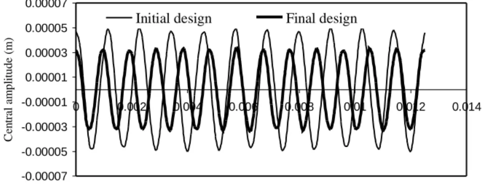
. The same optimal design is obtained using gradient optimization.The amplitudes and the natural frequencies of the plate in free vibrations, enabled by an applied uniform distributed transverse load q
= 10000 N/m2and then removed, are shown in Figure 1 for both the initial and final lamination sequences. As expected, for the final design, there is a decreasing in the central amplitude and the fundamental natural frequency increases.
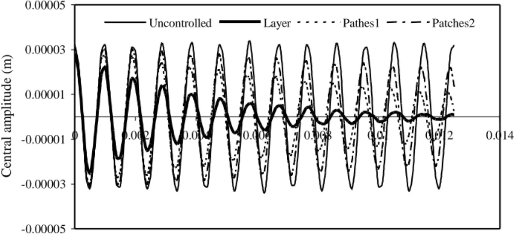
Next we pretend to investigate the optimal position of the piezoelectric actuators patches, in order to maximize the control of the plate, in this case measured by the amplitude of the deflection in the center of the plate, and compare it with the control obtained by using an entire piezoelectric layer. In this application, 4 actuators patches covering 8 triangular elements are introduced. The plate is modeled by a (6x6) element mesh (72 triangular elements). Using the simulating annealing algorithm the optimal positions of the patches is obtained as represented in Figure 2 a), i.e. the central plate elements (Patches 1). In Figure 2 a) and b) two different patches positions are shown, and the corresponding central line deflections, as well as those obtained with an entire actuator layer, are shown in Figure 3. Figure 4 illustrates the responses for central amplitude of the plate, and compares these responses in three different situations. The controlled responses, obtained using a time step ∆t=0.000125 s in the Newmark method, with
8000 G
Gi c = , clearly demonstrates the damping effect of the piezoelectric actuators on the free vibration of the plate with an
applied uniform distributed transverse load q = 10000 N/m2,which was then suddenly removed.
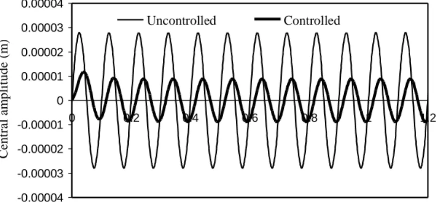
For an applied distributed transverse harmonic load q(t)=qsin 2πf t with a magnitude q=10000N and frequency f =10Hz, Figure 5 shows the uncontrolled and controlled responses, where the effect of negative velocity feedback control, GiGc=3.2×10⁷, is evident. -0.00007 -0.00005 -0.00003 -0.00001 0.00001 0.00003 0.00005 0.00007 0 0.002 0.004 0.006 0.008 0.01 0.012 0.014 Time (seconds) C en tr al a m p li tu d e (m )
Initial design
Final design
Figure 1. Central amplitude for the initial and final lamination sequence.
Figure 2 a). Patch locations – Patches 1.
y
Figure 2 b). Patch locations – Patches 2.
0 0.00001 0.00002 0.00003 0.00004 0.00005 0 0.03 0.06 0.09 0.12 0.15 0.18
Layer Patches1 Patches2
Figure 3. Central line deflections.
Figure 6 shows the relation of the amplitude of plate vibration versus feedback control gain G. It can be observed that the amplitude of plate vibration decreases quickly when the control gain increases up to approximately G=GiGc≈40 x (1.6 x 106), but then it decreases very slowly for higher values of G.
-0.00005 -0.00003 -0.00001 0.00001 0.00003 0.00005 0 0.002 0.004 0.006 0.008 0.01 0.012 0.014 Time (seconds) C en tr al a m p li tu d e (m )
Uncontrolled Layer Pathes1 Patches2
Figure 4. Uncontrolled and controlled responses on the plate central amplitude.
x
-0.00004 -0.00003 -0.00002 -0.00001 0 0.00001 0.00002 0.00003 0.00004 0 0.2 0.4 0.6 0.8 1 1.2 Time (seconds) C en tr al a m p li tu d e (m ) Uncontrolled Controlled
Figure 5. Uncontrolled central deflection, f =10 Hz
0 0.000005 0.00001 0.000015 0.00002 0.000025 0.00003 0 20 40 60 80 100
Feedback gain (1.6 x 10E-06)
C en tr al a m p li tu d e (m )
Figure 6. Amplitude vs. Feedback gain
-0.001 -0.0008 -0.0006 -0.0004 -0.0002 0 0.0002 0.0004 0.0006 0.0008 0.001 0 0.002 0.004 0.006 0.008 0.01 0.012 Time (seconds) C en tr al a m p li tu d e (m ) Uncontrolled GiGc=1.6x10E05 GiGc=0.32x10E05
Figure 7. Effect of negative velocity feedback control on the central deflection
For the same applied transverse harmonic load but now considering a frequency of f =1050Hz, which is very close to the first natural frequency, Figure 7 illustrates the uncontrolled and controlled responses for central deflection w. The controlled responses for gains GiGc=0.32 x 10⁵ and GiGc=1.6 x 10⁵, clearly demonstrates the action of the piezoelectric actuator layer, which increases
9. Conclusions
The active control capability of composite structures covered with piezoelectric layers or patches is investigated, using the finite element method. A finite element based on the Kirchhoff classical theory, has been developed. The present model has been validated in Moita et al. [26], where the solutions for deflection and sensed voltage in a bimorph beam, are compared with the solutions obtained by other authors. Here, the results obtained, show that the negative velocity feedback control algorithm used in this model is effective for an active damping control of vibration response. Also the core optimization had been performed in order to minimize the vibration amplitude and maximization of first natural frequency. The patch position optimization had been also performed in order to maximize the effect a defined set of actuators. Both of these optimizations used the simulated annealing method. Acknowledgments
The authors thank the financial support of Fundação Calouste Gulbenkian and POCTI/FEDER, Fundação para a Ciência e Tecnologia (FCT) and Projecto POCTI/FEDER/ EME/37559/2001.
References
1. Allik H, and Hughes T. Finite Element Method for Piezoelectric Vibration. Int. J. Num. Methods Eng, 1970, 2: 151-157. 2. Crawley E F and de Luis J. Use of Piezoelectric Actuators as Elements of Intelligent Structures. AAIA Journal, 1987, 25(10):
1373-1385.
3. Tzou H S and Tseng C I. Distributed Piezoelectric Sensor/Actuator Design for Dynamic Measurement/Control of Distributed Parametric Systems: A Piezoelectric Finite Element Approach. J. Sound Vibration, 1990, 138: 17-34.
4. Chen C Q, Wang X M, and Shen Y P. Finite element approach of vibration control using self-sensing piezoelectric actuators. Computers and Structures, 1996, 60 (3): 505-512.
5. Samanta B, Ray M C, and Bhattacharyya R. Finite element model for active control of intelligent structures. AIAA Journal, 1996, 34(9): 1885-1893.
6. Lam K Y, Peng X Q, Liu G R, and Reddy J N. A finite element model for piezoelectric composite laminates. Smart Material Structures, 1997, 6: 583-591.
7. Moita J S, Correia I F, Mota Soares C M, and Mota Soares C A. Active control of laminated structures with bonded piezoelectric sensors and actuators. Computers and Structures, 2004, 82: 1349-1358.
8. Bathe K J. Finite Element Procedures in Engineering Analysis. Prentice-Hall Inc, Englewood Cliffs, New Jersey, USA, 1982. 9. Franco V M, Gomes M A, Suleman A, Mota Soares C M, and Mota Soares C A. Modeling and design of adaptive composite
structures. Comp. Meth. Appl. Mech. Eng., 2000, 185: 325-346.
10. Benjeddou A. Advances in piezoelectric finite element modeling of adaptive structural elements: A survey. Computer and Structures, 2000, 76: 347-363.
11. Batra R C and Liang X Q. The vibration of a rectangular laminated elastic plate with embedded piezoelectric sensors and actuators. Computers and Structures, 1997, 63 (2): 203-216.
12. Liang C, Sun F P, and Rogers C A. Determination of design of optimal actuator location and configuration based on actuator power factor. J. Intell. Material Systems and Structures, 1995, 6: 456-464.
13. Franco Correia V M, Mota Soares C M, and Mota Soares C A. Refined models for the optimal design of adaptive structures using simulated annealing. Composite Structures, 2000, 54: 161-167.
14. Padula S L and Kincaid R K. Optimization strategies for sensor and actuator placement. NASA, Langley Research Center, Langley, Virginia 23681, 1999, 1-12.
15. Frecker M I. Recent advances in optimization of smart structures. Journal of Intelligent Material Systems and Structures, 2003, 14, (4-5): 207-216.
16. Atiqullah M M and Rao S S. Simulated annealing and parallel processing: an implementation for constrained global design optimization. Eng. Optimization, 2000, 32: 659-685.
17. Tiersten H F. Linear Piezoelectric Plate Vibrations. New York: Plenum Press, 1969.
18. Reddy J N. Mechanics of laminated composite plates. CRC Press, Boca Raton, New York, 2004.
19. Zienckiewicz O C. The Finite Element Method in Engineering Sciences. 3rd ed. London: McGraw-Hill, 1977. 20. Reddy J N. On laminate composite plates with integrated sensors and actuators. Engineering Structures, 1999, 21: 568-593. 21. Vanderplaats G N. Numerical optimization techniques for engineering design: with applications. New York: McGraw-Hill Inc.,
1994.
22. Herskovits J. A two stage feasible directions interior point technique for nonlinear optimization. J. Optim. Theory Appli., 1998, 99(1): 121-146.
23. Leite J P B and Topping B H V. Parallel simulated annealing for structural optimization. Computers and Structures, 1999,73: 545-564.
24. Franco Correia V, Mota Soares C M and Mota Soares C A. Refined models for the optimal design of adaptive structures using simulated annealing. Composite Structures, 2001, 54: 161-167.
25. Franco Correia V, Mota Soares C M and Mota Soares C A. Buckling optimization of composite laminated adaptive structures. Composite Structures, 2003, 62: 315-321.
26. Moita J S, Mota Soares C M, and Mota Soares C A. Geometrically non-linear Analysis of composite structures with integrated piezoelectric sensors and actuators. Composite Structures, 2002, 57, (1- 4): 253-261.