Finite element analysis of actively controlled smart plate with
patched actuators and sensors
Abstract
The active vibration control of smart plate equipped with patched piezoelectric sensors and actuators is presented in this study. An equivalent single layer third order shear de-formation theory is employed to model the kinematics of the plate and to obtain the shear strains. The governing equa-tions of motion are derived using extended Hamilton’s prin-ciple. Linear variation of electric potential across the piezo-electric layers in thickness direction is considered. The elec-trical variable is discretized by Lagrange interpolation func-tion considering two-noded line element. Undamped natural frequencies and the corresponding mode shapes are obtained by solving the eigen value problem with and without elec-tromechanical coupling. The finite element model in nodal variables are transformed into modal model and then recast into state space. The dynamic model is reduced for further analysis using Hankel norm for designing the controller. The optimal control technique is used to control the vibration of the plate.
Keywords
smart plate, FEM, sensors, actuators, vibration control, op-timal control, LQG.
M. Yaqoob Yasina,∗, Nazeer
Ahmadb and M. Naushad
Alama
aDepartment of Mechanical Engineering,
Ali-garh Muslim University, AliAli-garh. 202002 – In-dia
bStructural Division, ISRO, Bangalore, 560017
– India
Received 5 Jan 2010; In revised form 21 Jun 2010
∗Author email: [email protected]
1 INTRODUCTION
Study of hybrid composite laminates and sandwich structures, with some embedded or surface bonded piezoelectric sensory actuator layers, known as smart structures, have received signifi-cant attention in recent years especially for the development of light weight flexible structures. Distributed piezoelectric sensors and actuators are widely used in the laminated composite and sandwich plates for several structural applications such as shape control, vibration suppres-sion, acoustic control, etc. Embedded or surface bonded piezoelectric elements can be actuated suitably to reduce undesirable displacements and stresses. These laminated composites have excellent strength to weight and stiffness to weight ratios, so they are widely used to control the vibrations and deflections of the structures.
film as active element on a cantilevered beam, they were able to demonstrate active damping of the first vibrational mode. Crawley and de Luis [6] developed an induced strain actua-tor model for beams. They formulated static and dynamic analytical models based on the governing equations for beams with embedded and surface bonded piezoelectric actuators to model extension and bending. They presented the results for isotropic and composite can-tilever beams with attached and embedded piezoelectric actuators. The study suggest that segmented actuators are always more effective than continuous actuators since the output of each actuator can be individually controlled. They also showed that embedded actuators in composites degrade the ultimate tensile strength, but have no effect on the elastic modulus. Baz and Poh [3] investigated methods to optimize the location of piezoelectric actuators on beams to minimize the vibration amplitudes. The numerical results of the problem demon-strated the control for vibrations in large flexible structures. Im and Atluri [9] presented a more complete beam model, which accounted for transverse and axial deformations in addi-tion to extension and bending. Governing equaaddi-tions were formulated for a beam with bonded piezoelectric actuators for applications in dynamic motion control of large-scale flexible space structures. Crawley and Anderson [5] developed a model to accurately predict the actua-tion induced extension and bending in one-dimensional beams. The model neglected shear effects and best suited for the analysis of thin beams. Robbins and Reddy [18] developed a piezoelectric layer-wise laminate theory for beam element. The comparisons were made us-ing four different displacement theories (two equivalent sus-ingle layer theories and two layerwise laminate theories). Hwang and Park [8] presented finite element modeling of piezoelectric sensors and actuators which is based on classical plate theory. Classical theory for beams and plates has been used for active vibration control study of smart beams and plates by many researchers [10, 14, 19]. The classical theory used in these studies to model the structures is based on Kirchhoff-Love’s assumption and hence neglects the transverse shear deformation effects. First order shear deformation theory has been employed for active vibration control of smart beams and plates by [4, 11–13, 21]. This theory however include the effects of transverse shear deformation but require shear correction factors which is a difficult task for the study of smart composite structures with arbitrary lay-up. To overcome these drawbacks, Reddy [17] developed third order shear deformation theory for plates. Peng, et al [16] presented the finite element model for the active vibration control of laminated beams using consistent third order theory. Zhou et al. [24] presented coupled finite element model based on third order theory for dynamic response of smart composite plates. Few studies [7, 22] on active vibration control smart plates have been performed using 3D solid elements but the computation cost is high due to increased number of degrees of freedom.
perfectly collocated. The linear quadratic regulator (LQR) which does not require collocated actuator sensor pairs is employed for vibration control study for smart beams and plates [10– 12, 15, 21–23]. The main drawback of LQR control is that it requires the measurement of all the states variables. The linear quadratic Gaussian (LQG) controller which does not require the measurement of all the state variables and formed by employing an optimal observer along with the LQR is employed in very few studies, for e.g. [7] for active vibration control of smart plates.
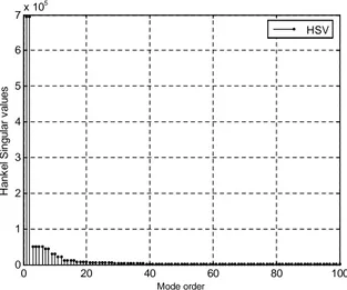
The objective of the present study is to present active vibration control of smart plate equipped with patched piezoelectric actuators and sensors. The governing equations of motion are derived using extended Hamilton’s principle. The discretization for finite element (FE) is done using four-node rectangular element which is based on third order theory. The electrical variable is discretized by Lagrange interpolation function considering two-noded line element. The resulting finite element equations in nodal variables are transformed into modal form and then recast into state space to design the controller. The dynamic model is reduced for further analysis using Hankel singular values. In this study, three steps have been used for the LQG design: (i) Designing of linear quadratic regulator (LQR) to obtain the control input based on measured state; (ii) Designing of linear quadratic estimator (Kalman observer) to provide an optimal estimate of the states; and (iii) Combine the separately designed optimal regulator and the Kalman filter into an optimal compensator, which generates the input vector based on the estimated state vector rather than the actual state vector, and the measured output vector.
2 MATHEMATICAL MODELING
2.1 Linear constitutive relations of piezoelectricity
The constitutive relations for material behavior of piezoelectric material considering electrome-chanical behavior can be expressed in tensor notations as follows [20]
εij =SijklE σkl+dkijEk, Di=diklσkl+bσijEj (1)
Or in semi inverted form as
σij =CijklE εkl−ekijEk, Di=eiklεkl+bεikEj (2)
where εij is strain tensor, Sijkl is elasticity compliance tensor, σij is stress tensor, dkij is
the piezoelectric strain constants, bij are the electric permitivities (di-electric tensor), Cijkl is
elastic constant tensor,ekij are piezoelectric stress constants,Di is electric displacement, and
Ek are electric field intensity components.
2.2 Derivation of governing equations
extended Hamilton’s principle
δ∫
t2
t1 (
T−U +Wc+Wnc)dt=0 (3)
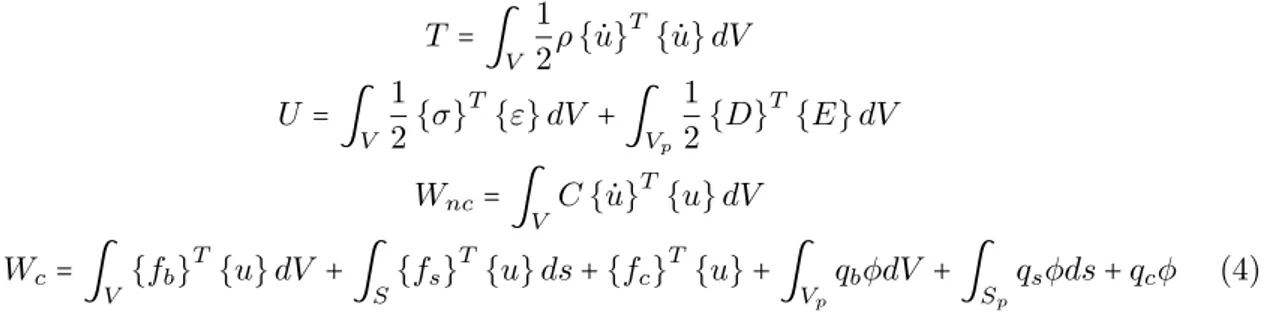
where T is the kinetic energy, U is the electromechanical potential energy (strain energy and electrical potential energy). WcandWncis the work done by external electrical and mechanical
conservative and non conservative forces, respectively. t1and t2are the time instants at which all first variations vanish. Various energy terms in equation (3) are defined as
T=∫
V
1 2ρ{u˙}
T
{u˙}dV
U =∫
V
1 2{σ}
T
{ε}dV + ∫
Vp
1 2{D}
T
{E}dV
Wnc=∫
V C{u˙} T{
u}dV
Wc=∫
V {fb} T
{u}dV + ∫
S{fs} T
{u}ds+{fc}T{u}+ ∫
VpqbφdV + ∫Spqsφds+qcφ (4)
whereV andVpdenote entire volume of the plate and volume of piezoelectric laminate/patches,
respectively, S and Sp represent the surface-boundary of the entire domain and piezoelectric
boundary, respectively, fb, fs and fc are the body force vector, surface tractions vector and
concentrated force vector, respectively. qb,qsandqcare body, surface and concentrated charge
distributions, respectively. C is material damping constant and u is displacement vector. Dot over a variable represents time derivative.
Figure 1 Surface bonded piezoelectric plate.
u(x, y, z)=u0(x, y)+zψx(x, y)−
4z3 3h2(ψx+
∂w0 ∂x )
v(x, y, z)=v0(x, y)+zψy(x, y)− 4z3
3h2(ψy+ ∂w0
∂y ) (5)
w(x, y, z)=w0(x, y)
where u0, v0 and w0 are the displacements of a point in the mid plane of laminate in the direction of x, y, and z respectively. ψx and ψyare the rotations of the transverse normal in
plane, z=0, about y and x axis respectively, h is the total thickness of the laminate. Strains are obtained by using the following relation from the above displacement field
εij=1/2(ui,j+uj,i) (6)
The electric potential function φ is assumed to vary linearly along the z direction and is constant in x and y directions in the piezoelectric layer and zero in rest of the portion. The piezoelectric layer contains metallic electrode on its top and bottom layers and thus they form equipotential surfaces. Grounding the surface atz=z1i.e. φ=0 and applying a voltageφ=φ1 atz=z2. The transverse variation is given as
φ=φ1(t) ( z−z1)
(z2−z1)
(7)
The electric field E is related with the electric potentialφ by the following relation
{E}=−{ ∂φ∂x ∂φ∂y ∂φ∂z }T (8) thus, we have
E=−⎧⎪⎪⎪⎪
⎨⎪⎪⎪ ⎪⎩
0 0 1 (z2−z1)
⎫⎪⎪⎪⎪ ⎬⎪⎪⎪ ⎪⎭
φ1 (9)
2.3 Finite element discretization
The smart composite plate is discretized into four noded rectangular elements. Each node has seven-degree of freedom i.e. { u0 v0 w0 ψx ψy ∂w∂x0 ∂w∂y0 }. Piezoelectric elements
contain one more electrical degree of freedom for every patch. The displacement variables u0, v0,ψx and ψy are expressed in terms of nodal variables using Lagrange interpolation functions of the four-node rectangular element and the electrical variable is discretized by Lagrange interpolation function of the two-node line element. While the transverse displacement variable
w0 is interpolated using Hermite interpolation.
[ M0 00 ] { u¨u
¨
uφ }+[
Cuu 0
0 0 ] {
˙
uu
˙
uφ }+[
Kuu Kuφ
Kφu Kφφ ] {
uu uφ }={
Fu
Fφ }
(10)
where M,Cuu and Kuu are mass, damping and stiffness matrices respectively, Kuφ and Kφu
are piezoelectric coupling matrices and Kφφ is the dielectric stiffness matrix. Fu and Fφ
denotes the mechanical and electrical load vectors respectively. uu anduφare mechanical and
electrical displacements respectively. Usually, proportional viscous damping in the model is assumed which is of the form
Cuu=αK+βM (11)
where αand β are constants to be determined experimentally.
The overall system Equation (10) can be rewritten in terms of generalized electrical poten-tial for sensors, uφs, and for actuators,uφa, as follows
⎡⎢ ⎢⎢ ⎢⎢ ⎣
M 0 0
0 0 0
0 0 0
⎤⎥ ⎥⎥ ⎥⎥ ⎦ ⎧⎪⎪⎪ ⎨⎪⎪⎪ ⎩ ¨ uu ¨ uφa ¨ uφs ⎫⎪⎪⎪ ⎬⎪⎪⎪ ⎭ +⎡⎢⎢⎢⎢⎢ ⎣
Cuu 0 0
0 0 0
0 0 0
⎤⎥ ⎥⎥ ⎥⎥ ⎦ ⎧⎪⎪⎪ ⎨⎪⎪⎪ ⎩ ˙ uu ˙ uφa ˙ uφs ⎫⎪⎪⎪ ⎬⎪⎪⎪ ⎭ +⎡⎢⎢⎢⎢⎢ ⎣
Kuu Kuφa Kuφs
KuφaT Kφφa 0
KuφsT 0 Kφφs
⎤⎥ ⎥⎥ ⎥⎥ ⎦ ⎧⎪⎪⎪ ⎨⎪⎪⎪ ⎩ uu uφa uφs ⎫⎪⎪⎪ ⎬⎪⎪⎪ ⎭ =⎧⎪⎪⎪⎨⎪⎪⎪ ⎩ Fu Fφa 0 ⎫⎪⎪⎪ ⎬⎪⎪⎪ ⎭ (12) sensor equation can be deduced from above as follows
KuφsT uu+Kφφsuφs=0
Mu¨u+Cuuu˙u+[Kuu−KuφsK−
1
φφsKuφsT ] u˙u={Fu}−Kuφauφa (13)
The equation (13) is modified in the form
Mu¨u+Cuuu˙u+Kmod uu={Fu}−Kuφauφa (14)
where, Kmod =[Kuu−KuφsK−1
φφsKuφsT ] is the modified stiffness of the host structure due to
piezoelectric effect.
2.4 The modal model
In the finite element model, the degrees of freedom of the system are quite large therefore it is required to model the system in modal form. The equation of motion for undamped free vibration can be extracted from finite element model, equation (14) for modal analysis as
Mu¨u+Kmoduu=0 (15)
The solution of this equation is of the form uu = U0ejωt where j =
√
corresponding eigen vector{ φ1 φ2 .... φn }. φigives theithnatural mode or mode shape.
The important property of the natural modes is that they are not unique and therefore they can be arbitrary scaled. Defining the matrix of the natural frequency as
Ω=diag( ω1 ω2 .... ωn ) (16)
and the modal matrix Φ which consists ofn natural modes of the system can be expressed as
Φ=[ φ1 φ2 .... φn ] (17)
Where each column of this matrix equation is the eigen vector corresponding to each of the eigen values. Since the mass, stiffness and damping matrices are symmetric, so the modal matrix normalized with respect to mass matrix diagonalizes these matrices as
Mm=ΦTMΦ=I, Km=ΦTKmodΦ=Ω2, Cm=ΦTCuuΦ=Λ (18)
hereMm,KmandCmare diagonal matrices known as modal mass, modal stiffness and modal
damping matrices respectively. I is an identity matrix. The diagonal modal damping matrix Λ with the generic term 2ξiωi, where ξi is the modal damping ratio and ωi the undamped
natural frequency of theith mode. The inclusion of the inherent damping effects in the model is considerably simplified due to the above method.
The governing system dynamics equation (14) is expressed in modal space by introducing a new variable derived by modal transformation
uu=Φq (19)
Pre-multiplying equation (14) by ΦT and employing equations (18) and (19), the second
order modal model can be written in its final form as
¨
q+Λ ˙q+Ω2q=ΦT[{Fu}−Kuφaueφa] (20)
The sensor equation can be written into modal space as
Kuφ sT Φq+Kφφsuφ s=0 (21)
3 ACTIVE VIBRATION CONTROL
3.1 Modal model in terms of state space
The system equation (20) can be written in terms of the state space as follows.
˙
x=Ax+Bu (22)
A=[ 0 I
−Ω Λ ], B=[
0 0
ΦT −ΦTK uφa ]
, u=[ Fu uφa ]
And the output equation that relates the sensor voltage generated over piezoelectric patches and its rate to states of the model is expressed as
y=Cx (23)
Where
C=[ −K −1
φφ sKuφ sT Φ 0
0 −K−1
φφ sKuφ sT Φ ]
3.2 Optimal control
In optimal control the feedback control system is designed to minimize the cost function, or performance index. It is proportional to the required measure of the system’s response and to the control inputs required to attenuate the response. The cost function can be chosen to be quadratically dependent on the control input
j=∫
T
0 [
xT(t)Qxx(t)+uT(t)Ru(t) ]dt (24)
Where Qx is a positive definite (or positive semi-definite) Hermitian or real symmetric
matrix known as state weighting matrix. R is a positive definite Hermitian or real symmetric matrix known as control cost matrix. There are several parameters which must be considered for the performance index (equation (24)). The first thing is that any control input which will minimizej will also minimize a scalar number timej. This is mentioned because it is common to find the performance index with a constant of ½ in front.
The second item to point out is in regard to the limits on the integral in the performance index. The lower limit is the present time, and the upper limit T is the final or terminal time. So the control input that minimizes the performance index will have some finite time duration, after which it will stop. This form of behavior represents the general case, and is applied in practice to cases such as missile guidance systems. In active sound and vibration control, we normally require a system, which will provide attenuation of unwanted disturbances forever. This corresponds to the special case of equation (24) where the terminal time is infinity.
j=∫
∞
0 [x
T(t)Q
xx(t)+uT(t)Ru(t) ]dt (25)
Equation (25) is referred to as a steady state optimal control problem, and is the form of the problem to which we will confine our discussion.
Two feedback control laws are available for controller design: state feedback and output feed-back. Linear quadratic regulator (LQR) is usually employed to determine the feedback gain. The feedback gain K is chosen to minimize a quadratic cost or performance index (PI) of equation (24). State feedbackLinear Quadratic Regulator (LQR) considered here is governed by the control law
u=−Gx (26)
The steady state feed back control gain K in equation (26) is given by
G=R−1BTP (27)
where P is the solution of the matrix Riccati equation
ATP+P A−P BR−1BTP+Qx =0. (28)
Finally it is assumed that all the states of the system are completely observable and there-fore directly related to the outputs of the system and used in the control system. But this is not always the case and more realistic approach is desired which consider that only the out put of the system can be known and measurable. Therefore, to incorporate the states information in the control system, it is necessary to estimate the states of the system from the model. The estimation of the states of the system is done by using Kalman Filter which is the state observer or state estimator.
In order to use Kalman filter to remove noise from a signal, the process must be such that it can be described by a linear system. The state equation for our system is modified to
˙
x=Ax+Bu+w (29)
and out put equation is given by
y=Cx+z (30)
where,wis called the process noise which may arise due to modeling errors such as neglecting non-linearities, z is called the measurement noise. The vector x contains all the information about the present state of the system. We cannot measure the statex directly so we measure y, which is a function of x and corrupted byz. We can now use the value ofy to estimate x, but we cannot get the full information about x from y due the presence of errors like noise which may be due to instrument errors. To control the systems with some feedback, we need accurate estimation of state variable x. The Kalman filter uses the available measurements y to estimate the states of the system. For that estimation we have the following requirements.
2. The variation between the state estimate and the true state should be as small as possible. So, we require an estimator with smallest possible error variance.
The above two requirements of the estimator are well satisfied by the Kalman filter. The assumptions about noise that affects the performance of our system are as follows. The mean of w and z should be zero and they are independent random variables, i.e. the noise should be a white noise. We define the noise covariance matrices Sw and Sz for process noise and
measurement noise covariance as
Sw=E{wkwTk}, Sz =E{zkzkT} (31)
The control law developed for the LQG controller is based on the estimation ˆxof the states
x of the system rather than the actual states of the system, which is given by
u=−Gkxˆ(t) (32)
Where, Gk is the gain of the Kalman estimator and is obtained by
Gk =M CTS−
1
z (33)
Where M is the again the solution of another steady state matrix Riccati equation
M AT+AM +Sw−M CTS−
1
Z CM =0 (34)
The dynamic behavior of the Kalman estimator is given by the following first order linear differential equations
˙ˆ
x=Axˆ+Bu+Gk(Cx+z−Cxˆ)
˙
e=(A−GkC)e+w−Gkz (35)
Due to the presence of w and z, the estimation error is not converges to zero, but it would remains as small as possible by proper selection of Gk.
Thus the controlled LQG closed loop can take the final form
˙
x=(A−BG)x+BGe+w
˙
e=(A−GkC)e−Gkz+w
(36)
or in matrix form,
{ xe˙˙ }=[ A−0BG A−BGG
kC ]{
x e }+[
I 0
I −Gk ]{
w
z } (37)
And the system’s output is
4 NUMERICAL RESULTS
4.1 Validation of numerical code and comparison
For the validation of the MATAB code developed for the finite element analysis of the piezo-electric plate, we solved the simple benchmark static problem of Hwang and Park [8] and compared the results obtained with the published results.
In this case, we consider a bimorph cantilever plate made of two layers of PVDF which are pooled in ± z direction. The length of the width of the laminate is 100 mm and 5 mm respectively and the thickness of each lamina is 0.5 mm. The configuration of elastic PVDF bimorph is labeled in figure 2, which is fixed on one side and free at the other side. The physical dimensions and material properties of the bimorph are listed in the table 1.
Figure 2 Woo-Seok Hwang and Hyun Chul Park problem.
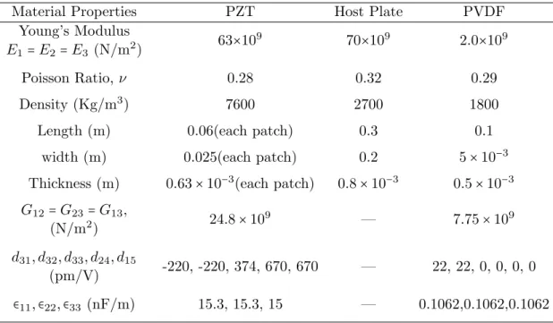
Table 1 Material properties and dimensions.
Material Properties PZT Host Plate PVDF
Young’s Modulus
E1=E2=E3 (N/m 2
) 63×10
9
70×109
2.0×10⁹
Poisson Ratio, ν 0.28 0.32 0.29
Density (Kg/m3
) 7600 2700 1800
Length (m) 0.06(each patch) 0.3 0.1
width (m) 0.025(each patch) 0.2 5×10⁻³
Thickness (m) 0.63×10⁻³
(each patch) 0.8×10⁻³
0.5×10⁻³
G12=G23=G13, (N/m2
) 24.8×10
9
— 7.75×10⁹
d31, d32, d33, d24, d15
(pm/V) -220, -220, 374, 670, 670 — 22, 22, 0, 0, 0, 0
∈11,∈22,∈33 (nF/m) 15.3, 15.3, 15 — 0.1062,0.1062,0.1062
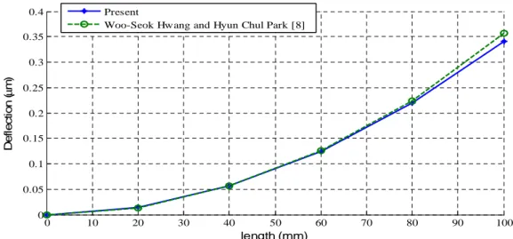
is calculated and compared with the published results given in reference [8]. The variation of tip deflection for different applied potentials is studied and the results and presented in figure 3 along with Hwang’s work. Figure 4 shows the variation of tip deflection for different applied potentials across the bimorph. It can be observed from these plots that the results obtained are in excellent agreement with those presented in the reference. Therefore it can be used for further analysis with confidence.
0 10 20 30 40 50 60 70 80 90 100
0 0.05 0.1 0.15 0.2 0.25 0.3 0.35 0.4
length (mm)
D
e
fl
e
c
ti
o
n
(
µ
m
)
Present
Woo-Seok Hwang and Hyun Chul Park [8]
Figure 3 Beam deformation for 1 volt, applied across the thickness.
0 20 40 60 80 100 120 140 160 180 200
0 1 2 3 4 5 6 7x 10
-5
Voltage applied across the bimorph (volt)
T
ip
d
e
fl
e
c
ti
o
n
(
m
)
Woo-Seok Hwang and Hyun Chul Park [8] Present
4.2 Numerical example
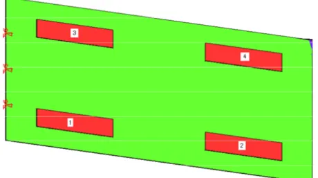
A rectangular aluminum cantilever plate with four rectangular PZT patches, bonded to the top surface of the plate, are used as actuators and four other PZT patches bonded symmetrically to bottom surface are to be used as sensor, forming four sets of collocated actuator-sensor pairs. The configuration is depicted in figure 5. The material properties and geometrical dimensions of the host plate and PZT layers are listed in the table 1. The problem domain has been descritized in 160 rectangular identical elements as shown in figure 6.
Figure 5 Configuration of smart cantilever plate with piezoelectric patches.
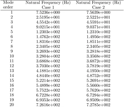
The modal analysis has been performed for two cases;
Case 1. The piezoelectric patches are short circuited thereby rendering ineffective the
piezo-electric coupling effect that enhances the stiffness of otherwise passive structure. This case includes the pure structural stiffness of the PZT patches and modal analysis involves the solution of following Eigen value problem.
∣Kuu−ω2M∣=0
Since the patches are short circuited, no electrical potential across them will build up due to deformation that reduces the coupling terms to zero.
Case 2. In this case, all 8 PZT patches are acting as sensor hence modifying the eigen value
problem as,
∣Kmod−ω
2
M∣=0 Where Kmod=[Kuu−KuφsK−
1
φφsKuφsT ]
Point 1 Point 2 Point 4
Point 3
Figure 6 Plate geometry with FEM grids. Table 2 First twenty natural frequencies of the plate.
Mode order
Natural Frequency (Hz) Natural Frequency (Hz)
Case 1 Case 2
1 7.5236e+000 7.5639e+000
2 2.5195e+001 2.5221e+001
3 4.5542e+001 4.5591e+001
4 9.0215e+001 9.0371e+001
5 1.2303e+002 1.2310e+002
6 1.4762e+002 1.4956e+002
7 1.8316e+002 1.8511e+002
8 2.3405e+002 2.3405e+002
9 3.2693e+002 3.2818e+002
10 3.2804e+002 3.3568e+002
11 3.6868e+002 3.6872e+002
12 3.7030e+002 3.7819e+002
13 4.1881e+002 4.1950e+002
14 4.8440e+002 4.8752e+002
15 5.2214e+002 5.2691e+002
16 5.4899e+002 5.5660e+002
17 5.7522e+002 5.7620e+002
18 6.7228e+002 6.7294e+002
19 6.9353e+002 6.9509e+002
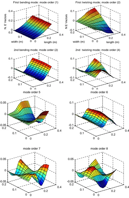
0 0.2 0.4 0 0.1 0.2 0 0.2 0.4 length (m) First bending mode: mode order (1)
width (m) N . E V e c to rs 0 0.2 0.4 0 0.1 0.2 -0.1 0 0.1 length (m) First twisting mode; mode order (2)
width (m) N E V e c to rs 0 0.2 0.4 0 0.1 0.2 -0.1 0 0.1
2nd bending mode; mode order (2)
0 0.2 0.4 0 0.1 0.2 -0.1 0 0.1
2nd twisting mode; mode order (4)
0 0.2 0.4 0 0.1 0.2 -0.05 0 0.05
mode order 5
0 0.2 0.4 0 0.1 0.2 -0.1 0 0.1
mode order 6
0 0.2 0.4 0 0.1 0.2 -0.05 0 0.05
mode order 7
0 0.2 0.4 0 0.1 0.2 -0.05 0 0.05
mode order 8
Figure 7 Mode shapes of PZT plates.
0 20 40 60 80 100 0
1 2 3 4 5 6
7x 10
5
Mode order
H
a
n
k
e
l
S
in
g
u
la
r
v
a
lu
e
s
HSV
Figure 8 Hankel Singular values for FE model.
4.3 Design of LQG controller
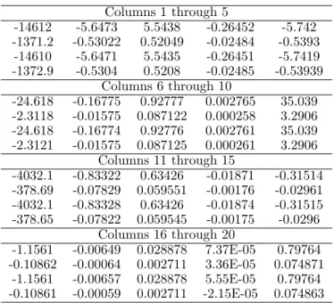
The ultimate aim of a feedback control system is to achieve the maximum control over the system dynamics keeping in view of hardware limitations. The 5 inputs, 4 piezoelectric ac-tuators and one mechanical point force and 4 outputs, the 4 piezoelectric sensors constitute the MIMO system shown in figure 5. The LQG regulator consists of two parts an optimal controller and a state estimator (Kalman observer). The controller gain is calculated by opti-mizing the functional of equation (25). The optimal gain matrix which is obtained from the solution of the matrix Riccati equation for a choice of state weighing matrix Q as diagonal matrix whose first element is 1012
and the remaining elements are unity. This choice is to give priority to control the first mode. Control effort matrix, R, is chosen 100×I where I
is an identity matrix. This value is chosen in such a way to keep the actuator voltage under the specified limit. The linear quadratic optimal gain matrix is presented in table 3 which shows that the entries of the optimal gains matrix for columns 1 and 11 which correspond to first mode for modal displacements and velocities are larger than other entries correspond to remaining modes, which indicate that the designed controller is more effective for controlling the vibrations for first mode but can effectively control the vibrations for other modes also. The entries of optimal gain matrix in rows 1 and 3 which correspond inputs through actuators 1 and 3 are larger (about 10 times) for all modes as compared with the entries for inputs through actuator 2 and 4. This indicates that more control effort is needed at actuator 1 and 3 for controlling the vibration of the plate. All calculations have been done using MATLAB 7.1.
The Kalman filter design is based on 4 noisy measured outputs of the sensors and five inputs to the system that includes 4 actuators and one mechanical point force input on tip of cantilever plate. Measured outputs and inputs are subjected to White Gaussian noise having variance of 1×10⁻⁴
N2
for mechanical input channel and 1 volt2
Table 3 Optimal Gain Matrix,G.
Columns 1 through 5
-14612 -5.6473 5.5438 -0.26452 -5.742
-1371.2 -0.53022 0.52049 -0.02484 -0.5393
-14610 -5.6471 5.5435 -0.26451 -5.7419
-1372.9 -0.5304 0.5208 -0.02485 -0.53939
Columns 6 through 10
-24.618 -0.16775 0.92777 0.002765 35.039
-2.3118 -0.01575 0.087122 0.000258 3.2906
-24.618 -0.16774 0.92776 0.002761 35.039
-2.3121 -0.01575 0.087125 0.000261 3.2906
Columns 11 through 15
-4032.1 -0.83322 0.63426 -0.01871 -0.31514
-378.69 -0.07829 0.059551 -0.00176 -0.02961
-4032.1 -0.83328 0.63426 -0.01874 -0.31515
-378.65 -0.07822 0.059545 -0.00175 -0.0296
Columns 16 through 20
-1.1561 -0.00649 0.028878 7.37E-05 0.79764
-0.10862 -0.00064 0.002711 3.36E-05 0.074871
-1.1561 -0.00657 0.028878 5.55E-05 0.79764
-0.10861 -0.00059 0.002711 -2.15E-05 0.074863
Table 4 Steady state Kalman gain matrix,Gk.
-0.000608 -5.7093e-005 -0.000608 -5.7089e-005
-1.2557e-007 -1.1804e-008 -1.2557e-007 -1.1803e-008
-1.4368e-005 -4.5093e-005 -1.4368e-005 -4.5094e-005
-3.0759e-009 -7.952e-010 -3.0759e-009 -7.952e-010
9.8185e-006 -8.0229e-006 9.8182e-006 -8.023e-006
7.9915e-006 -7.3316e-006 7.9915e-006 -7.3316e-006
-9.434e-010 5.5201e-011 -9.434e-010 5.5209e-011
-1.1325e-007 -7.7762e-008 -1.1325e-007 -7.7789e-008
8.774e-010 8.3681e-010 8.774e-010 8.3681e-010
-7.4606e-006 -7.2951e-006 -7.4606e-006 -7.2951e-006
-0.0036009 -0.0018818 -0.0036009 -0.0018818
-7.6714e-007 -3.9994e-007 -7.6713e-007 -3.9995e-007
0.00024819 -0.0011062 0.00024817 -0.0011062
-1.5123e-008 -2.0148e-008 -1.5123e-008 -2.0148e-008
0.0012739 -0.0023066 0.0012739 -0.0023066
-0.0006839 -0.00014206 -0.00068389 -0.00014206
3.1234e-009 5.5673e-009 3.1235e-009 5.5673e-009
0.0010656 0.00046203 0.0010656 0.00046204
5.7711e-008 -8.8099e-010 5.7711e-008 -8.7879e-010
-0.00040051 0.00011638 -0.00040051 0.00011636
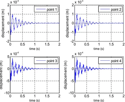
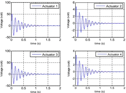
After obtaining the controller and observer gain matrix now system is exited with given initial condition. Initial condition vector is derived by deforming the plate by a 0.5 N force in the direction of z at mid of the tip. Deflection thereby obtained is transformed into modal space using weighted modal matrix. That in turn has been used as initial condition modal displacement vector with conjunction of zero modal velocities. The various parameters of system response are presented in figures 9-12. Points are shown on grid whose time history is presented in figure 6. Sensor and actuator voltages on S/A pairs (1, 3) is higher than the S/A pairs (2, 4) because of their nearness to fixed end thereby having large strains. Since the plate was excited in such a way that the first bending mode was dominating the system behavior and for that reason, a large state weight was attributed to the element that corresponds to the 1st mode in state weighing matrixQ. From Figure 12 one can infer that first mode is decaying faster than other modes.
0 0.5 1 1.5 2
-2 -1 0 1
2x 10
-3 time (s) d is p la c e m e n t (m )
0 0.5 1 1.5 2
-2 -1 0 1
2x 10
-3 time (s) d is p la c e m e n t (m )
0 0.5 1 1.5 2
-10 -5 0
5x 10
-4 time (s) d is p la c e m e n t (m )
0 0.5 1 1.5 2
-10 -5 0
5x 10
-4 time (s) d is p la c e m e n t (m ) point 2 point 1
point 3 point 4
Figure 9 Displacement time histories of selected points.
5 CONCLUSIONS
0 0.5 1 1.5 2 -50 0 50 100 time (s) V o lt a g e ( v o lt )
0 0.5 1 1.5 2
-4 -2 0 2 4 6 time (s) V o lt a g e ( v o lt )
0 0.5 1 1.5 2
-50 0 50 100 time (s) V o lt a g e ( v o lt )
0 0.5 1 1.5 2
-4 -2 0 2 4 6 time (s) V o lt a g e ( v o lt ) Actuator 4
Actuator 1 Actuator 2
Actuator 3
Figure 10 Control voltages applied on actuators vs. time history.
0 0.5 1 1.5 2
-4 -2 0 2 4 time (s) v o lt a g e ( v o lt )
0 0.5 1 1.5 2
-1 -0.5 0 0.5 1 time (s) v o lt a g e ( v o lt )
0 0.5 1 1.5 2
-4 -2 0 2 4 time (s) v o lt a g e ( v o lt )
0 0.5 1 1.5 2
-1 -0.5 0 0.5 1 time (s) v o lt a g e ( v o lt ) Sensor 1 Sensor 3 Sensor 2 Sensor 4
0 0.2 0.4 0.6 0.8 1 1.2 1.4 1.6 1.8 2 -5
0 5x 10
-4
M
o
d
e
1
0 0.2 0.4 0.6 0.8 1 1.2 1.4 1.6 1.8 2 -2
0 2x 10
-7
M
o
d
e
2
0 0.2 0.4 0.6 0.8 1 1.2 1.4 1.6 1.8 2 -1
0 1x 10
-5
M
o
d
e
3
Figure 12 Modal displacement time histories.
model the dynamic behavior and control strategies for vibration of smart structures with piezoelectric actuators and sensors.
The natural frequencies of vibration are obtained with and without electromechanical cou-pling. It is observed that electromechanical coupling effect is more effective for lower frequen-cies. Since most of the energy is associated with the first few modes, therefore these modes only need to be controlled. As observed from plots, the control model is quite effective. The designed LQG controller is quite useful for multi-input-multi-output (MIMO) systems.
References
[1] R. Alkhatib and M. F. Golnaraghi. Active structural vibration control: a review. Shock and Vibration Digest,
35(5):367–383, 2003.
[2] T. Bailey and J. E. Hubbard. Distributed piezoelectric-polymer active vibration control of a cantilever beam.Journal
of Guidance, 8:605–611, 1985.
[3] A. Baz and S. Poh. Performance of an active control system with piezoelectric actuators. Journal of Sound and
Vibration, 126:327–343, 1988.
[4] G. Caruso, S. Galeani, and L. Menini. Active vibration control of an elastic plate using multiple piezoelectric sensors
and actuators.Simulation Modelling Practice and Theory, 11:403–419, 2003.
[5] E. F. Crawley and E. H. Anderson. Detailed models of piezoceramic actuation of beams. Journal of Intelligent
Material Systems and Structures, 1:4–25, 1990.
[6] E. F. Crawley and J. de Luis. Use of piezoelectric actuators as elements of intelligent structures. AIAA Journal,
25:1373–1385, 1987.
[7] X-J. Dong, G. Meng, and J-C. Peng. Vibration control of piezoelectric smart structures based on system identification
technique: Numerical simulation and experimental study.Journal of Sound and Vibration, 297:680–693, 2006.
[8] W. S. Hwang and H. C. Park. Finite element modeling of piezoelectric sensors and actuators. AIAA Journal,
31:930–937, 1993.
[9] S. Im and S. N. Atluri. Effects of a piezo-actuator on a finitely deformed beam subjected to general loading. AIAA
[10] T-W. Kim and J-H. Kim. Optimal distribution of an active layer for transient vibration control of a flexible plate. Smart Materials and Structures, 14:904–916, 2005.
[11] K. R. Kumar and S. Narayanan. The optimal location of piezoelectric actuators and sensors for vibration control of
plates. Smart Materials and Structures, 16:2680–2691, 2007.
[12] Z. K. Kusculuoglu and T. J. Royston. Finite element formulation for composite plates with piezoceramic layers for
optimal vibration control applications. Smart Materials and Structures, 14:1139–1153, 2005.
[13] G. R. Liu, K. Y. Dai, and K. M. Lim. Static and vibration control of composite laminates integrated with piezoelectric
sensors and actuators using radial point interpolation method.Smart Materials and Structures, 14:1438–1447, 2004.
[14] J. M. S. Moita, I. F. P. Correia, C. M. M. Soares, and C. A. M Soares. Active control of acaptive laminated structures
with bonded piezoelectric sensors and actuators. Computers and Structures, 82:1349–1358, 2004.
[15] S. Narayanan and V. Balamurugan. Finite element modelling of piezolaminated smart structures for active vibration
control with distributed sensors and actuators.Journal of Sound and Vibration, 262:529–562, 2003.
[16] X. Q. Peng, K. Y. Lam, and G. R. Liu. Active vibration control of composite laminated beams with piezoelectrics:
a finite element model with third order theory.Journal of Sound and Vibration, 209:635–650, 1997.
[17] J. N. Reddy. A simple higher-order theory for laminated composite plates. ASME Journal of Applied Mechanics,
51:745–752, 1984.
[18] D. H. Robbins and J.N. Reddy. Analysis of piezoelectrically actuated beams using a layer-wise displacement theory. Computers and Structures, 41:265–279, 1991.
[19] K. Umesh and R. Ganguli. Shape and vibration control of smart plate with matrix cracks. Smart Materials and
Structures, 18:1–13, 2009.
[20] S. Valliappan and K. Qi. Finite element analysis of a smart damper for seismic structural control. Computers and
Structures, 81:1009–1017, 2003.
[21] C. M. A. Vasques and J. D. Rodrigues. Active vibration of smart piezoelectric beams: Comparison of classical and
optimal feedback control strategies. Computers and Structures, 84:1459–1470, 2006.
[22] S. X. Xu and T. S. Koko. Finite element analysis and design of actively controlled piezoelectric smart structure. Finite Elements in Analysis and Design, 40:241–262, 2004.
[23] A. Zabihollah, R. Sedagahti, and R. Ganesan. Active vibration suppression of smart laminated beams using layerwise
theory and an optimal control strategy.Smart Materials and Structures, 16:2190–2201, 2007.
[24] X. Zhou, A. Chattopadhyay, and H. Gu. Dynamic response of smart composites using a coupled