http://dx.doi.org/10.1590/S1982-21702017000300031
Article
PROPOSAL OF THE SPATIAL DEPENDENCE EVALUATION FROM
THE POWER SEMIVARIOGRAM MODEL
Proposta de avaliação da dependência espacial a partir do modelo de
semivariograma potência
Ismael Canabarro Barbosa 1
Edemar Appel Neto 1
Enio Júnior Seidel 1
Marcelo Silva de Oliveira 2
1Universidade Federal de Santa Maria (UFSM) - Santa Maria – RS – Brasil. E-mail: [email protected]; [email protected]; [email protected]
2Universidade Federal de Lavras (UFLA) - Lavras – MG – Brasil. E-mail: [email protected]
Abstract:
In Geostatistics, the use of measurement to describe the spatial dependence of the attribute is of great importance, but only some models (which have second-order stationarity) are considered with such measurement. Thus, this paper aims to propose measurements to assess the degree of spatial dependence in power model adjustment phenomena. From a premise that considers the equivalent sill as the estimated semivariance value that matches the point where the adjusted power model curves intersect, it is possible to build two indexes to evaluate such dependence. The first one, SPD*, is obtained from the relation between the equivalent contribution (α) and the equivalent sill (C* = C0 + α), and varies from 0 to 100% (based on the calculation of spatial dependence areas). The second one, SDI*, beyond the previous relation, considers the equivalent factor of model (FM*), which depends on the exponent that describes the force of spatial dependence in the power model (based on spatial correlation areas). The SDI*, for close to 2, assumes its larger scale, varying from 0 to 66.67%. Both indexes have symmetrical distribution, and allow the classification of spatial dependence in weak, moderate and strong.
Keywords: Geostatistics; Variographic analysis; Semivariogram without sill; Spatial dependence
indexes.
Resumo:
potência. A partir de uma premissa que considera o patamar-equivalente como o valor de semivariância que coincide com o ponto em que as curvas ajustadas do modelo potência se interceptam, pode-se construir dois índices para avaliação de tal dependência. O primeiro, DE*, é obtido a partir da relação entre a contribuição-equivalente (α) e o patamar-equivalente (C* = C0 +
α), e varia de 0 a 100% (baseado no cálculo de áreas de dependência espacial). O segundo, IDE*, além da relação anterior, considera um fator de modelo equivalente (FM*), que depende do expoente , o qual descreve a força da dependência espacial no modelo potência (baseado em áreas de correlação espacial). O IDE*, para próximo de 2, assume sua maior escala, variando de 0 a 66.67%. Ambos os índices possuem distribuição simétrica, e permitem a classificação da dependência espacial em fraca, moderada e forte.
Palavras-chave: Geoestatística; Análise variográfica; Semivariogramas sem patamar; Índices de
dependência espacial.
1. Introduction
In geostatistics applications, in general, the spatial dependence (or spatial autocorrelation) is assessed by the semivariogram study, which is the most important tool for such evaluation (Seidel, Oliveira, 2013; 2014a). This method requires expertise and time from the researcher, since it is not always easy to visualize the shape of the semivariogram model that best fits the data.
Among the models capable of adjustment bythe semivariogram, the most used are the spherical, exponential and Gaussian (Lourenço, Landim, 2005; Seidel, Oliveira, 2013). These models feature sill, in other words, they comply with the second-order stationarity, having four parameters: nugget effect, contribution, sill and range.
According to Seidel, Oliveira (2014a), for being a descriptor with plenty of graphic details, the semivariogram generates a lot of information, making it necessary to construct a numerical auxiliary measure of the spatial dependence. Such measure may summarize the entire set of semivariographic information to complement the semivariogram study. Besides that, according to Biondi, Myers, Avery (1994), spatial dependence measures are important to compare phenomena (different spatial dependence scenarios) because they assess the degree of dependence.
In the literature from Geosciences and Rural Sciences, some indexes evaluate the spatial dependence degree in models with evident sill (second-order stationarity). There may be mentioned the Relative Nugget Effect (NE) (Trangmar, Yost, Uehara, 1985; Cambardella et al., 1994) and the Spatial Dependence Degree (SPD) (Biondi, Myers, Avery, 1994), considering, respectively, the following relations between the parameters of the semivariogram: nugget effect (C0) and sill (C0 + C1); contribution (C1) and sill (C0 + C1). These two indexes to evaluate the spatial dependence are used by many studies, for example, Barbieri et al. (2013), Costa et al. (2013), Kamimura et al. (2013), Neves Neto et al. (2013), Peluco et al. (2013), Santos, H. et al. (2013), Santos, M. et al. (2013), Nascimento et al. (2014), Lundgren, Silva, Ferreira (2015), Rocha et al. (2015).
2014b), can be understood as a value that expresses the strength of spatial dependence that the model can achieve.
However, when models that do not reach a sill are fitted, as far as it is known, there is no proposed spatial dependence measures, because the ones presented in the literature consider this parameter in their formulations. From this moment, when we refer to models that do not reach sill, we will mention just as models without sill. Thus, to contemplate situations of non-second-order stationarity, we justifythe attempt to create spatial dependence measures to semivariograms with fitted models without sill. Therefore, in this study, measures to assess the spatial dependence degree on phenomena with power model adjustment are proposed.
2. Methodology
The index named relative nugget effect (NE) (Trangmar, Yost, Uehara, 1985; Cambardella et al., 1994) relates the nugget effect and the sill and is given by the expression:
0 0 1
(%) C 100
NE
C C
(1)
where C0 is the nugget effect and C1 is the contribution. According to Cambardella et al. (1994), the NE(%) can be classified as follows: strong spatial dependence from 0 to 25%, moderate spatial dependence from 25 to 75%, and weak spatial dependence from 75 to 100%.
The measure proposed by Biondi, Myers, Avery (1994), in which contribution and sill are related, is denominated spatial dependence (SPD) and is given by:
1 0 1
(%) C 100
SPD
C C
(2)
where C0 is the nugget effect and C1 is the contribution. Adapting theclassification of Cambardella et al. (1994), the SPD(%) index is defined by: weak spatial dependence from 0 to 25%, moderate spatial dependence from 25 to 75%, and strong spatial dependence from 75 to 100%.
1 0 1
(%) 100
Model
C a
SDI FM
C C q MD
(3)
where C0 is the nugget effect, C1 is the contribution, a is the range, FM is the factor of model and MD is the maximum distance between pairs of sample points. In the validation study of SDI, Seidel, Oliveira (2014a) considered q = 0.5, generating a denominator qMD equivalent to half the greater distance between sample points.
It is possible to observe that the indexes presented previously are applicable only in second-order stationarity models, whose sill has been reached. However, the power model has no such feature, making it impossible the direct indexes application as they are defined.
The power model, featuring stationarity only under intrinsic hypothesis, is given as (Olea, 2006):
0
( )h C h
, 0 2 , 0 (4)
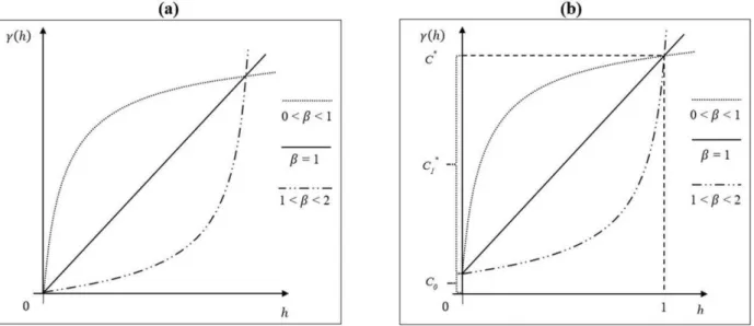
where C0 is the nugget effect, α is the inclination (or slope), is the power (or exponent), and h is the distance between points. Graphically, the model can be seen in Figure 1a.
Figure 1: (a) Power semivariogram model; (b) Configuration of the premisse in which C1*=α.
The only parameter contained in the indexes expressed in the Equations 1, 2 and 3 and set in the power model in the Equation 4, is the nugget effect parameter. That way, from the power model it is necessary to create equivalent parameters that simulate the behavior of the sill, contribution and range parameters, making it possible to apply spatial dependency indexes in this model.
assumption considers that the equivalent sill may be equal to the semivariance value in which the theoretical curves of the power model intersect (see Figure 1b).
The first assumption was inspired by the fact that, in models with sill, there is similarity between the sample variance and the sample sill (Trangmar, Yost, Uehara, 1985; Lima, G. et al., 2014; Nagahama et al., 2014; Lima, J. et al., 2014; Jordão et al., 2015). So that, it was considered as possible to extend this idea to the power model, turning the sample variance approximately equal to the value of sample equivalent sill, in other words, the sample variance could be considered as the estimate of the equivalent sill.
In this approach, the equality is considered: equivalent sill (C*) = sample variance (S²). From this equality, the relationship is defined:
estimated equivalent sill (�̂∗) = estimated nugget effect (�̂ ) + estimated equivalent contribution
(�̂∗)
sample variance (S²) = estimated nugget effect (�̂ ) + estimated equivalent contribution (�̂∗). Thus, understanding that the estimated equivalent contribution is equal to a value W, such as: W = S² - �̂ , it is possible to observe that the applicability of this approach has the restriction that S² must be greater or equal to the estimated nugget effect (S² ≥ �̂ ).
Furthermore, the estimated equivalent range (�̂∗) is the value of the distance (h) with the estimated
semivariance [ (h)] equal to the sample variance (S²), that is, the estimated equivalent range (�̂∗) is the value of the distance (h), such as: �̂ + αh = S².
This assumption, based on equality between the estimated equivalent sill and the sample variance, has weaknesses in its application, because it depends on the occurrence of the S² ≥ �̂ condition. This condition may not always really occur and does not depend on the spatial behavior of the studied phenomenon, since the value of S² depends only on the sampling distribution of the phenomenon. Thus, in this article, the calculation of indexes from this approach is not developed. Jia et al. (2009) presents the possibility of considering the value of 95% of the highest semivariance obtained in the semivariogram sample as an equivalent value to a sill, in linear and power models. This approach also seems to be arbitrary, because it is not necessarily that this 95% cut of the semivariogram would be the best estimate of an equivalent sill. For this reason, it will not be developed in this article.
The second possible approach is more general and always applicable because it depends only on the elements of spatial behavior of the phenomenon under study. This approach is based on the assumption that the equivalent sill can be assessed as the value of the estimated semivariance [ (h)] that coincides with the point at which the adjusted power model curves intersect. Graphically, the justification for this second approach is illustrated in Figure 1b. On this assumption, the estimated equivalent sill (�̂∗) is equal to the value of (h) for which h is equal to 1. That means, �̂∗ = �̂ +
̂. From this equality, the relation is defined as:
estimated equivalent sill (�̂∗) = estimated nugget effect (�̂ ) + estimated equivalent contribution (�̂∗)
To find the value of h where the curves of model intersect, it is only necessary to equal two equations of them. Next, it is possible to check for any case of two arbitrary (0 < ≤ 1 e 1≤
< 2), with ≠ :
1( )h 2( )h
1 2
1 2
ˆ ˆ
0 1 0 2
ˆ ˆ ˆ ˆ
C h C h
Where
1 2
0 0
ˆ ˆ
C C e ˆ1 ˆ2
therefore,
1 2
ˆ ˆ
h h
For this equality be true, h = 0 or h = 1. As the curves visually are in h = 0, in the origin of the semivariogram (see Figure 1), then the non-zero result found is h = 1. Thus,
ˆ ˆ
*
0 0 0
ˆ ˆ ˆ ˆ ˆ1 ˆ ˆ
C C h C C (5)
The next subsection of the article deals with the construction of the SPD* index, from the approach of estimation of equivalent sill with the intersection of the power model curves. This index is constructed in an attempt to, in cases of power model application, imitate the SPD index proposed by Biondi, Myers, Avery (1994), which is applied in cases of models with sill.
2.1 The Construction of the
SPD
*index
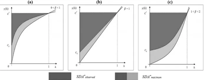
The SPD* index is calculated based on an adaptation of the concept of spatial dependence areas (Seidel, Oliveira, 2014b; 2015). The index is obtained as the ratio between the equivalent observed spatial dependence area (SDA*observed) and the equivalent maximum spatial dependence area (SDA*maximum) as the following expression:
* *
* *
* 0
*
* * max
0
{ ( )}
(%) 100 100
{ }
a
observed
a imum
C h dh
SDA SPD
SDA C C h dh
where SDA*observed is given as the integral of the difference between equivalent sill and the power model; the SDA*maximum is given as the integral of the difference between equivalent sill and the adapted power model (C0 = 0). Both integrals are defined between zero and equivalent range. Figure 2 shows the equivalent spatial dependence observed and maximum areas.
Figure 2: Equivalent observed and maximum spatial dependence areas for the power model with
(a) 0 < < 1; (b) = 1; (c) 1 < < 2.
In the next subsection, the proposed construction of the SDI* index is described. This index is built in an attempt to, in cases of power model application, imitate the SDI index proposed by Seidel, Oliveira (2014a), which is applied in cases of models with sill.
2.2 The Construction of the
SDI
*index
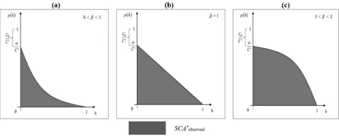
The SDI* index is constructed from an adaptation of the concept of spatial correlation areas (Seidel, Oliveira, 2014a). Here, the SDI* index, built from the calculation of equivalent observed spatial correlation area, can be described by the expression:
*
* *
* 0
1 ( ) 1
(%) observed 100 a 1 100
h
SDI SCA dh
q MD C q MD
(7)Figure 3: Equivalent observed spatial correlation area for the power model with (a) 0 < < 1;
(b) = 1; (c) 1 < < 2.
2.3 Indexes classification
At this stage of the study, it is developed the categorization of indexes to enable the classification of spatial dependence in terms of weak, moderate and strong, based on the classification suggested by Cambardella et al. (1994) for NE(%) index. The intention is to perform the categorization making two cuts in the distribution of index values, the first in the value corresponding to the 1st quartile, and the second to the 3rd quartile, similarly from Cambardella et al. (1994), which proposed cuts in the value 25% (value of the 1st quartile) and value 75% (value of the 3rd quartile) for an index which had distribution of values ranging from 0 to 100%.
After this, to show the validity and applicability of the indexes, the real data from articles in which the power model was used, was applied in the study. Then, the indexes were calculated and the spatial dependence was classified.
3. Results and discussion
From the premise that the value of the equivalent sill (C*) is given by C0 + α, wherein a*= 1, the SPD* index calculation is given as follows:
* *
* *
* 1 *
* *
*
0
* 0 0
* * 1 *
* * * * * *
max
0 0
( ) ( ) 1
( )
1
a a
observed
a a
imum
a a
C h dh C C h dh
SDA SPD
C a
SDA C C h dh C C h dh C a
Placing αa* in evidence in the numerator and C*a* in the denominator, there is:
* * 1
* *
* * 1 *
* * * * 1 1 1 1 1 1 a a a a
C a a
C a C a
Taking a*=1, there is:
0
0 1 1 1 1 1 1 C C
Thus, there is:
* 0 (%) 100 SPD C (8)
where C0 is the nugget effect and α is the slope coefficient (equivalent contribution).
This index assumes values from 0 to 100%, analogously to the SPD(%) index given by Biondi, Myers, Avery (1994). Thus, the same way that in SPD(%) index, it is assumedthat the SPD*(%) index has symmetric distribution and it can be classified according to the same principle applied to the SPD(%) index, adapting the classification of Cambardella et al. (1994). Therefore, the classification of SPD*(%) is:
▪ 0 ≤ SPD*(%) ≤ 25% → Weak spatial dependence
▪ 25% < SPD*(%) ≤ 75% → Moderate spatial dependence
▪ 75% < SPD*(%) ≤ 100% → Strong spatial dependence
On the assumption used for the construction of SPD* (C* = C0 + α) and utilizing the methodology of SDI index proposed by Seidel, Oliveira (2014a), it is possible to develop the calculation of SDI* index as follows:
*
* *
* 0
1 ( ) 1
1
a
observed
h
SDI SCA dh
q MD C q MD
* * * * 1
* * *
0
( ) 1 1
1
a C h a a
dh
C q MD C C q MD
Placing �∗∗ in evidence, there is:
* * * 1 1 1 a a
C q MD
Taking a*=1, there is:
*
1 1
1
1
C q MD
As a* = 1, it does not make sense to keep the correction factor
�� , since it does not have the
effect of equivalent range in the expression of SDI*. Thereby, there is:
* 0 1 1 1 1 1 1 C C
Finally, there is:
*
0 1
(%) 1 100
1 SDI C
(9)
where C0 is the nugget effect, α is the slope coefficient (equivalent contribution) and is the exponent. The term 1 −
+ is the equivalent factor of model (FM
*) of the power model.
Then, it is observed that the FM* for the power model depends only on the parameter. Thus, for 0 < < 1 there is 0 < FM* < 0.500. For = 1 there is FM* = 0.500. And, for 1 < < 2 there is 0.500 < FM* < 0.667. This makes the index assume values from 0 to FM*×100%. For example, in the case of power model with = 1, the value of SDI*(%) can vary in the range between 0 and 0.500×100%, that is, between 0 and 50%.
For the construction of the theoretical distribution of SDI* it is considered 101 values of component
0+ : sequence from 0 to 1, with variation 0.01. As the power model varies the scale of its
distribution depending on the value of , FM* has different possible values. Thus, for each possible value of , the 101 generated values are multiplied by FM*×100% to generate the specific distribution of SDI*, corresponding to each possible power model behavior. Figure 4 shows box plots of distributions of the theoretical values for some situations. In Figure 4a there is an example of distribution of the SDI*(%) values for FM* = 0.400 (0 < FM* < 0.500; 0 < < 1). Figure 4b shows the distribution of SDI*(%) when FM* = 0.500 ( = 1). And the Figure 4c shows the behavior of SDI*(%) for FM* = 0.600 (0.500 < FM* < 0.667; 1 < < 2).
Figure 4: Box plot of distribution of the theoretical values of SDI*(%) for: (a) FM*=0.4;
(b) FM*=0.5; (c) FM*=0.6.
The classification of SDI*(%) is performed based on the distribution of theoretical values, in each power model behavior (variation of ), as a set of data that is desired to categorize into three levels: weak, moderate, and strong spatial dependence. To do this, we calculate the first and third quartile with the intention to categorize the SDI*(%) inspired by the classification of Cambardella et al. (1994), applied to indexes with symmetrical behavior, which has cuts in 25% and 75% corresponding to cuts in the 1st and 3rd quartiles, respectively. Thus, for the SDI*(%), which also has symmetrical behavior as seen in Figure 4, the cuts are also made in the values corresponding to these two quartiles. That way, generalizing to any FM* (any ), the classification of the SDI*(%) is given as:
▪ 0 ≤ SDI*(%) ≤ 0.25×FM*×100% → Weak spatial dependence
▪ 0.25×FM*×100% < SDI*(%) ≤ 0.75×FM*×100% → Moderate spatial dependence
▪ 0.75×FM*×100% < SDI*(%) ≤ FM*×100% → Strong spatial dependence
To illustrate this classification, there were taken as an example, the values of the factors of model used for the construction of the box plot in Figure 4. For the FM*=0.400, weak spatial dependence
12.5% < SDI* ≤ 37.5% and the strong spatial dependence for 37.5% < SDI*≤ 50%. Finally, for the FM*=0.600 weak spatial dependence when 0 ≤ SDI* ≤ 15%, moderate spatial dependence for 15% < SDI* ≤ 45% and strong spatial dependence when 45% < SDI*≤ 60% were detected.
As varies in the power model, the FM* consequently varies its distribution. This behavior is different from the factors of model to the spherical, exponential and Gaussian models, which are fixed in each model, assuming, respectively, the values 0.375, 0.317 and 0.504 (Seidel, Oliveira, 2014a; 2014b; 2015). The maximum FM* that can be obtained in the power model is close to 0.667 (when is close to 2). This value is the highest among the semivariogram models already discussed (spherical, exponential, Gaussian and power).
The expression of SDI* index (Equation 9), as generated in this article, can be understood as the product of FM* and the SPD* index (Equation 8), that is, SDI* = FM*×SPD*. In other words, the SDI* index is analogous to SDI2 index obtained by Seidel, Oliveira (2015), for the spherical, Gaussian and exponential models, from a geometrical perspective of semivariogram.
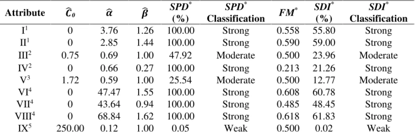
To exemplify the applicability of the SPD* and SDI* indexes, so that researchers can use them in their future studies, the real data obtained from some geosciences and rural sciences articles (Pardo-Igúzquiza, 1998; Makkawi, 2004; Jorge, 2009; Masseran et al., 2012; Shah, Patel, 2012) were taken in order to calculate the indexes and classify the spatial dependence. These articles present power model adjustment in the semivariogram to estimate the spatial dependence. And this application is presented in Table 1.
Table 1: Estimates of the power model parameters, SPD*, FM*, SDI* and spatial dependence
classification as exemplification in real data.
Attribute �̂0 ̂ ̂
SPD*
(%)
SPD*
Classification FM
* SDI*
(%)
SDI*
Classification
I1 0 3.76 1.26 100.00 Strong 0.558 55.80 Strong
II1 0 2.85 1.44 100.00 Strong 0.590 59.00 Strong
III2 0.75 0.69 1.00 47.92 Moderate 0.500 23.96 Moderate
IV2 0 0.66 0.27 100.00 Strong 0.213 21.26 Strong
V3 1.72 0.59 1.00 25.54 Moderate 0.500 12.77 Moderate
VI4 0 47.47 1.55 100.00 Strong 0.608 60.78 Strong
VII4 0 43.64 0.94 100.00 Strong 0.485 48.45 Strong
VIII4 0 68.84 1.62 100.00 Strong 0.618 61.83 Strong
IX5 250.00 0.12 1.00 0.05 Weak 0.500 0.02 Weak
IPre monsoon season in India; IIPost monsoon season in India; IIIWind Speed in East Malaysia; IVWind Speed in
Peninsular Malaysia; VSpatial dimension of shallow groundwater; VIPiezometric levels; VIIRainfall in Malaga
(Spain); VIIIPiezometric heads; IXSoil erosion in Botucatu-SP; 1Shah, Patel (2012); 2Masseran et al. (2012); 3Makkawi (2004); 4Pardo-Igúzquiza (1998); 5Jorge (2009).
4. Conclusion
Two new indexes for measuring the spatial dependence when using the power semivariogram model are proposed and justified from geostatistical arguments: the SPD* and SDI* indexes. The SPD* has symmetric distribution, holding scale of values ranging from 0 to 100%. The classification of Cambardella et al. (1994) can be applied to this index.
The SDI* also features symmetrical distribution. However, its scope depends on the value of FM* and consequently on the parameter. This index can be rated from 1st (0.25×FM*×100) and 3rd quartiles (0.75×FM*×100).
Both indexes generate the same spatial dependence classification. However, the use of SDI* index allows the evaluation of the strength of spatial dependence, as regards the factor of model.
For both indexes, the spatial dependence classification can be made considering the levels: weak, moderate and strong spatial dependence.
This study was performed as a proposal to index creation for the evaluation of spatial dependence in models that do not reach sill, comparing with already existing indexes in the literature for second-order stationarity models. Thus, as a preliminary work, it is necessary more researches and applications about this topic, making it possible further comparisons, verifying the applicability and reliability of the proposed indexes.
REFERENCES
Barbieri, D. M., Marques Júnior, J., Pereira, G. T., Scala Jr, N. L., Siqueira, D. S., Panosso, A. R. 2013. Comportamento dos óxidos de ferro da fração argila e do fósforo adsorvido, em diferentes sistemas de colheita de cana-de-açúcar. Revista Brasileira de Ciência do Solo, 37(6), pp.1557-1568.
Biondi, F., Myers, D. E., Avery, C. C. 1994. Geostatistically modeling stem size and increment in an old-growth forest. Canadian Journal of Forest Research, 24(7), pp.1354-1368.
Cambardella, C. A., Moorman, T. B., Novak, J. M., Parkin, T. B., Karlen, D. L., Turco, R. F.; Konopka, A. E. 1994. Field-scale variability of soil properties in Central Iowa soils. Soil Science Society of America Journal, 58(5), pp.1501-1511.
Costa, C. S., Pedrosa, E. M. R., Rolim, M. M., Santos, H. R. B., Cordeiro Neto, A. T. 2013. Effects of vinasse application under the physical attributes of soil covered with sugarcane straw. Engenharia Agrícola, 33(4), pp.636-646.
Jia, Z., Davis, E., Muzzio, F. J., Ierapetritou, M. G. 2009. Predictive modeling for Pharmaceutical processes using kriging and response surface. Journal of Pharmaceutical Innovation, 4(4), pp.174-186.
Jordão, W. H. C., Zanchi, F. B., Ferreira, D. M. M., Pagani, C. H. P., Luizão, F. J., Neves, J. R. D., Duarte, M. L. 2015. Variabilidade do índice de área foliar em campos naturais e floresta de transição na região Sul do Amazonas. Revista Ambiente e Água, 10(2), pp.363-375.
Kamimura, K. M., Santos, G. R., Oliveira, M. S., Dias Junior, M. S., Guimarães, P. T. G. 2013. Variabilidade espacial de atributos físicos de um latossolo vermelho-amarelo, sob lavoura cafeeira. Revista Brasileira de Ciência do Solo, 37(4), pp.877-888.
Lima, G. C., Silva, M. L. N., Oliveira, M. S., Curi, N., Silva, M. A., Oliveira, A. H. 2014. Variabilidade de atributos do solo sob pastagens e mata atlântica na escala de microbacia hidrográfica. Revista Brasileira de Engenharia Agrícola e Ambiental, 18(5), pp.517-526.
Lima, J. S. S., Bona, D. A. O., Fiedler, N. C., Pereira, D. P. 2014. Distribuição espacial das frações granulométricas argila e areia total em um latossolo vermelho-amarelo. Revista Árvore, 38(3), pp.513-521.
Lourenço, R. W., Landim, P. M. B. 2005. Mapeamento de áreas de risco à saúde. Cadernos de Saúde Pública, 21(1), pp.150-160.
Lundgren, W. J. C., Silva, J. A. A., Ferreira, R. L. C. 2015. Estimação de volume de madeira de eucalipto por cokrigagem, krigagem e regressão. Cerne, 21(2), pp.243-250.
Makkawi, M. H. 2004. Integrating GPR and geostatistical techniques to map the spatial extent of a shallow groundwater system. Journal of Geophysiscs and Engineering, 1(1), pp.56-62.
Masseran, N., Razali, A. M., Ibrahim, K., Wan Zin, W. Z., Zaharim, A. 2012. On spatial analysis of Wind energy potential in Malaysia. WSEAS Transactions on Mathematics. 11(6), pp.467-477. Nagahama, H. J., Cortez, J. W., Concenço, G., Araujo, V. F., Honorato, A. C. 2014. Dinâmica e variabilidade espacial de plantas daninhas em sistemas de mobilização do solo em sorgo forrageiro. Planta Daninha, 32(2), pp.265-274.
Nascimento, P. S., Silva, J. A., Costa, B. R. S., Bassoi, L. H. 2014. Zonas homogêneas de atributos do solo para o manejo de irrigação em pomar de videira. Revista Brasileira de Ciência do Solo, 38(4), pp.1101-1113.
Neves Neto, D. N., Santos, A. C., Santos, P. M., Melo, J. C., Santos, J. S. 2013. Análise espacial de atributos do solo e cobertura vegetal em diferentes condições de pastagem. Revista Brasileira de Engenharia Agrícola e Ambiental, 17(9), pp.995-1004.
Olea, R. A. 2006. A six-step practical approach to semivariogram modeling. Stochastic Environmental Research and Risk Assessment, 20(5), pp.307-318.
Pardo-Igúzquiza, E. 1998. MLREML4: Program for the inference of the power variograma model by maximum likelihood and restricted maximum likelihood. Computers & Geosciences, 24(6), pp.537-543.
Peluco, R. G., Marques Júnior, J., Siqueira, D. S., Pereira, G. T., Barbosa, R. S., Teixeira, D. B., Adame, C. R., Cortez, L. A. 2013. Suscetibilidade magnética do solo e estimação da capacidade de suporte à aplicação de vinhaça. Pesquisa Agropecuária Brasileira, 48(6), pp.661-672.
Rocha, F. C., Oliveira Neto, A. M., Bottega, E. L., Guerra, N., Rocha, R. P., Vilar, C. C. 2015. Weed mapping using techniques of precision agriculture. Planta Daninha, 33(1), pp.157-164. Santos, H. L., Marques Júnior, J., Matias, S. S. R., Siqueira, D. S., Martins Filho, M. V. 2013. Erosion factors and magnetic susceptibility in different compartments of a slope in Gilbués-PI, Brazil. Engenharia Agrícola, 33(1), pp.64-74.
Seidel, E. J., Oliveira, M. S. 2013. Proposta de uma generalização para os modelos de semivariogramas exponencial e gaussiano. Semina: Ciências Exatas e Tecnológicas, 34(1), pp.125-132.
Seidel, E. J., Oliveira, M. S. 2014a. Novo índice geoestatístico para a mensuração da dependência espacial. Revista Brasileira de Ciência do Solo, 38(3), pp.699-705.
Seidel, E. J., Oliveira, M. S. 2014b. Proposta de um teste de hipótese para a existência de dependência espacial em dados geoestatísticos. Boletim de Ciências Geodésicas, 20(4), pp.750-764.
Seidel, E. J., Oliveira, M. S. 2015. Medidas de dependência espacial baseadas em duas perspectivas do semivariograma paramétrico. Ciência e Natura, 37(4), pp.20-27.
Shah, J. A., Patel, H. R. 2012. Characterizing spatial variability of groundwater levels using semivariogram. International Journal of Civil Engineering, 4(1), pp.65-69.
Trangmar, B. B., Yost, R. S., Uehara, G. 1985. Application of geostatistics to spatial studies of soil properties. Advances in Agronomy, 38, pp.45-94.