Optical thickness and effective radius of Arctic boundary-layer clouds retrieved from airborne spectral and hyperspectral radiance measurements

(1)

AMTD

5, 7753–7781, 2012

Optical thickness and e_ffective radius

of Arctic clouds

E. Bierwirth et al.

Title Page

Abstract Introduction

Conclusions References

Tables Figures

◭ ◮

Back Close

Full Screen / Esc

Printer-friendly Version Interactive Discussion

Discussion

P

a

per

|

Dis

cussion

P

a

per

|

Discussion

P

a

per

|

Discussio

n

P

a

per

|

Atmos. Meas. Tech. Discuss., 5, 7753–7781, 2012 www.atmos-meas-tech-discuss.net/5/7753/2012/ doi:10.5194/amtd-5-7753-2012

Atmospheric Measurement Techniques Discussions

This discussion paper is/has been under review for the journal Atmospheric Measurement Techniques (AMT). Please refer to the corresponding final paper in AMT if available.

Optical thickness and e

_ff

ective radius of

Arctic boundary-layer clouds retrieved

from airborne spectral and hyperspectral

radiance measurements

E. Bierwirth1, A. Ehrlich1, M. Wendisch1, J.-F. Gayet2, C. Gourbeyre2, R. Dupuy2, A. Herber3, R. Neuber4, and A. Lampert4,*

1

University of Leipzig, Institute for Meteorology, Leipzig, Germany 2

Universit é Blaise Pascal, Laboratoire de M ét éorologie Physique, Aubi ère, France 3

Alfred Wegener Institute for Polar and Marine Research, Bremerhaven, Germany 4

Alfred Wegener Institute for Polar and Marine Research, Potsdam, Germany *

now at: Institute of Aerospace Systems, TU Braunschweig, Germany

Received: 1 October 2012 – Accepted: 9 October 2012 – Published: 23 October 2012 Correspondence to: E. Bierwirth (eike.bierwirth@uni-leipzig.de)

(2)

AMTD

5, 7753–7781, 2012

E. Bierwirth et al.

Title Page

Tables Figures

◭ ◮

Back Close

Full Screen / Esc

Discussion

P

a

per

|

Dis

cussion

P

a

per

|

Discussion

P

a

per

|

Discussio

n

P

a

per

|

Abstract

Arctic boundary-layer clouds in the vicinity of Svalbard (78◦N, 15◦E) were observed with airborne remote sensing and in situ methods. The cloud optical thickness and the droplet effective radius are retrieved from spectral radiance data in nadir and and from hyperspectral radiances in a 40◦field of view. Two approaches are used for the spectral

5

retrieval, combining the signal from either two or five wavelengths. Two wavelengths are found to be sufficient for an accurate retrieval of the cloud optical thickness, while the retrieval of droplet effective radius is more sensitive to the method applied. The comparison to in situ data cannot give a definite answer as to which method is better because of unavoidable time delays between the in situ measurements and the

remote-10

sensing observations.

1 Introduction

The Arctic is strongly affected by global warming (Walsh et al., 2011), and clouds play an integral part in the ongoing changes (Wu and Lee, 2012). However, satellite ob-servations are often obstructed by the low contrast between clouds and the surface

15

covered by snow or sea ice (Krijger et al., 2011), and airborne or ground-based cloud observations are scarce, especially over the Arctic Ocean.

The understanding of Arctic clouds is crucial to predict their role in greenhouse warm-ing (McBean et al., 2005). The Arctic heatwarm-ing trend was reported to continue in 2011 (Overland et al., 2011). The relationships between atmospheric conditions and the

mi-20

crophysical characteristics of mixed-phase clouds are key questions of cloud physics (Korolev and Isaac, 2006; de Boer et al., 2010; Seifert et al., 2010). Moreover, the microphysical characteristics of clouds (particle phase, size, concentration and shape) determine their radiative properties and, thus, their impact on the Earth’s radiation bud-get (Curry et al., 1996; Ehrlich et al., 2008a). This is of particular interest in the Arctic

25

where boundary-layer clouds greatly influence the surface radiation budget, as shown

(3)

AMTD

5, 7753–7781, 2012

E. Bierwirth et al.

Title Page

Tables Figures

◭ ◮

Back Close

Full Screen / Esc

Discussion

P

a

per

|

Dis

cussion

P

a

per

|

Discussion

P

a

per

|

Discussio

n

P

a

per

|

by Shupe and Intrieri (2004) from ground-based remote-sensing observations, and cli-mate change is particularly strong.

Verification of space-borne retrievals of cloud properties critically depends on inde-pendent airborne or ground-based measurements. Problems in retrievals arise from both instrument uncertainty and the assumptions made in the radiative transfer models

5

used for the retrieval algorithms (Brest et al., 1997; Marshak et al., 2006). Thus, cred-ible verification of remotely inferred cloud properties requires (i) direct comparison to in situ measurements; and (ii) comparison of spectral radiances simulated by radiative transfer models to measured quantities (Formenti and Wendisch, 2008; Barker et al., 2011).

10

For the purpose of improving the data base of the Arctic climate system, the SoRPIC (Solar Radiation and Phase Discrimination of Arctic Clouds) campaign was conducted in the Norwegian Arctic, including one of the first applications of an AisaEAGLE hyper-spectral camera for cloud studies. SoRPIC was a collaboration of the Alfred Wegener Institute for Polar and Marine Research (AWI), the University of Leipzig (Germany), the

15

Blaise Pascal University of Clermont-Ferrand (France), the Free University of Berlin (Germany), and the German Aerospace Center DLR. The measurement platform was the Polar-5 research aircraft (C-GAWI) of AWI, Bremerhaven (Germany). This Basler BT67 aircraft is a former DC-3 modernized by Basler Turbo Conversion Oshkosh (Wis-consin, USA) with modern avionics and navigation systems, and turbo prop engines

20

required for the demands of polar research. It was put in service in 2007 (Herber et al., 2008). With an operational range of 1500 km, a maximum altitude of 7.5 km (24 000 feet), 15 kVA of electrical power, and a weight capacity of 2000 kg, the Polar-5 provides a reliable platform for the study of boundary-layer clouds in the Arctic. It is based out of Bremerhaven, Germany, and is presently operated by Kenn Borek Air

25

Ltd., Calgary (Alberta, Canada).

(4)

AMTD

5, 7753–7781, 2012

E. Bierwirth et al.

Title Page

Tables Figures

◭ ◮

Back Close

Full Screen / Esc

Discussion

P

a

per

|

Dis

cussion

P

a

per

|

Discussion

P

a

per

|

Discussio

n

P

a

per

|

The term spectral without prefix refers to non-imaging measurements that yield two-dimensional datasets (time and wavelength).

2 Measurements

During the SoRPIC campaign which was held in Svalbard (Arctic Norway) between 30 April and 20 May 2010, a total of 13 research flights were conducted with the

Polar-5

5 aircraft over the Greenland, Norwegian, and Barents Seas.

The aircraft was equipped with a combination of remote-sensing and cloud-particle in situ instruments, listed in Table 1. Parts of the instrumentation are introduced in a recent book by Wendisch and Brenguier (2013). The remote-sensing equipment for this study included one active (the Airborne Mobile Aerosol Lidar AMALi; Stachlewska

10

et al., 2010) and three passive systems (the Spectral Modular Airborne Radiation Mea-surement System (SMART-Albedometer); AisaEAGLE; Sun photometer). The hyper-spectral imaging camera (AisaEAGLE, manufacturer: Specim Spectral Imaging Ltd., Oulu, Finland) was mounted in a tail-pod to measure upwelling radiancesI_λ↑_,E(t,y) as a function of wavelengthλ, timet, and cross-track distancey (subscript E for

AisaEA-15

GLE). The AisaEAGLE covers the spectral range from 403 nm to 966 nm in 240 chan-nels, with a resolution (full width at half maximum) of 2–3 nm. The cross-track field of view was 40◦wide, divided into 512 spatial pixels (1024 photo diodes with double bin-ning). A dark measurement for correction of the thermal photo-current in the detector was performed every five minutes. An exposure time of 10 ms was used.

20

During all flights, the upwelling radianceI_λ↑_,S(t,yn) from the nadir pointyn was

mea-sured by the SMART-Albedometer (subscript S), which also meamea-sured spectral down-welling and updown-welling irradiances,F_λ↓(t) andF_λ↑(t). The upwelling radiance reflected by the cloud is detected by an optical inlet with a field of view (FOV) of 1.5◦; the irradiance by integrating spheres (Crowther, 1997). The collected photons are guided by fibre

op-25

tics to grating spectrometers (manufactured by Zeiss, Jena/Germany; Bierwirth et al.,

(5)

AMTD

5, 7753–7781, 2012

E. Bierwirth et al.

Title Page

Tables Figures

◭ ◮

Back Close

Full Screen / Esc

Discussion

P

a

per

|

Dis

cussion

P

a

per

|

Discussion

P

a

per

|

Discussio

n

P

a

per

|

2009) with 1280 channels for wavelengths from 350 to 2100 nm. An exposure time of 500 ms was used.

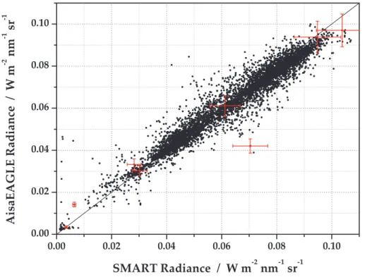
The viewing geometry for AisaEAGLE and SMART-Albedometer radiances is visual-ized in Fig. 1.

Both the AisaEAGLE and the SMART-Albedometer have an own Inertial Navigation

5

System (INS) that records the aircraft attitude (roll, pitch, and heading angles). Using these attitude data, the optical inlets of the SMART-Albedometer are actively horizon-tally stabilised to correct for changes of the aircraft attitude of up to 6◦with an accuracy of 0.2◦(Wendisch et al., 2001). The AisaEAGLE is fixed to the fuselage, so the real-time attitude angles have to be taken into account in data analysis.

10

The AisaEAGLE and the SMART-Albedometer were calibrated in the laboratory with a NIST-traceable standard bulb for irradiances and with a NIST-traceable integrating sphere for radiances. The calibration stability during the campaign was monitored with a portable integrating sphere, and was better than 3 %. The radiometric uncer-tainty is given as 8 % for the AisaEAGLE and 9 % for the SMART-Albedometer

radi-15

ance. The radiometric calibration of AisaEAGLE has been verified by comparing the upwelling radiances with that of the well-established SMART-Albedometer (compare Ehrlich et al., 2012). Using the INS attitude records, the AisaEAGLE pixels that are located in the field of view of the SMART-Albedometer’s radiance sensor are identi-fied for each time step. In this paper, such pixels are referred to as ES (the overlap is

20

shown in Fig. 1). The mean value of all ES pixels is used for comparing AisaEAGLE and SMART-Albedometer radiance data, as in Fig. 2 for a wavelength of 870 nm. The linear correlation coefficient in Fig. 2 is 0.97; the differences can be attributed not only to the measurement uncertainty but also to the different time resolution (1–2 Hz for the SMART-Albedometer, 35 Hz for the AisaEAGLE).

25

(6)

AMTD

5, 7753–7781, 2012

E. Bierwirth et al.

Title Page

Tables Figures

◭ ◮

Back Close

Full Screen / Esc

Discussion

P

a

per

|

Dis

cussion

P

a

per

|

Discussion

P

a

per

|

Discussio

n

P

a

per

|

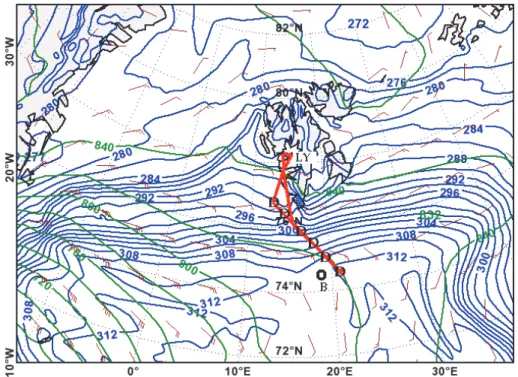
3 Meteorological situation on 17 May

On 17 May 2010, a warm front approached Svalbard from Scandinavia, with unusually high temperatures up to 14◦C (Fig. 3). The warm, dry air (50 % relative humidity) was advected onto a ridge of about 0◦C which remained under an inversion at the ocean surface. As observed by AMALi and the drop sondes (Fig. 4), both the inversion and

5

the cloud top increased in altitude toward north. The maximum temperatures ranged from 14◦C at 800 m (74.5◦N) to 8◦C at 1200 m altitude (75.9◦N). A cloud layer formed in the inversion. On the aircraft, we observed that these clouds had a foggy appearance and reached down to the ocean surface. This is supported by the Bjørnøya sounding (50 km west of the southern end of the flight track) that reports continuous saturation

10

up to 975 hPa (Dietzsch, 2010). The Cloud Particle Imager was not operational on this flight. An additional higher cloud layer at 1500 m was observed to the north of the warm airmass, and is excluded from the following discussions.

The aircraft flew at 3100 m altitude almost parallel to the temperature gradient (Fig. 3). Six drop sondes were launched; their data can be trusted only below 2900 m

15

after their adjustment to ambient conditions. AMALi could detect only the cloud top due to saturation.

4 Retrieval of cloud properties from spectral radiance

The cloud properties are retrieved from the spectral and hyperspectral radiance mea-surements aboard the Polar 5 aircraft. The measured data are checked against

look-20

up tables (LUT) of simulated radiances. These look-up tables are produced with the radiative transfer package libRadtran (Mayer and Kylling, 2005). The radiative transfer calculations are initialised with environmental parameters from the SoRPIC campaign, including Sun/aircraft geometry, aerosol optical thickness from the Sun photometer, cloud-top height from the AMALi lidar, and meteorological profiles from drop sondes

25

released from the aircraft. The look-up tables then contain the possible values for the

(7)

AMTD

5, 7753–7781, 2012

E. Bierwirth et al.

Title Page

Tables Figures

◭ ◮

Back Close

Full Screen / Esc

Discussion

P

a

per

|

Dis

cussion

P

a

per

|

Discussion

P

a

per

|

Discussio

n

P

a

per

|

spectral upward radiance in dependence on optical thickness τ and droplet effective radiusreffof a plane-parallel cloud, from which the most likely combination is obtained

by interpolation of the measured radiance into the simulated radiance grid.

Two approaches have been followed to retrieve the cloud optical properties (op-tical thickness, e_ffective radius) from spectral nadir radiance measurements by the

5

SMART-Albedometer. First, the two-wavelength approach (2WL) presented by Naka-jima and King (1990) is used with the radiance at 515 nm and 1625 nm. The grid of pre-calculated radiancesILUT is interpolated to the actual measured radianceImeas at

these wavelengths. Second, a five-wavelength (5WL) residual approach presented by Coddington et al. (2010) is followed. The same look-up tables are used, but analysed at

10

five wavelengths of 515, 745, 870, 1015, 1240, and 1625 nm in terms of the residuum

ζ2:

ζ2=

5

X

i=1

"

(5−i)2·(Ii,meas−Ii,LUT)2+(i−1)2·

I

i,meas

I_0,meas − I_i,LUT

I_0,LUT 2#

, (1)

where the index i runs over the five wavelengths in increasing order. The weighting factors in Eq. (1) reflect the wavelength dependence of the radiance sensitivity to optical

15

thickness (left term) and e_ffective radius (right term). Each of the five wavelengths represents a different order of magnitude of the bulk absorption coefficient of liquid water and, adding the dependence on droplet size, different ranges of single-scattering albedo (Coddington et al., 2010, Fig. 2). For any given flight geometry,ζ2is calculated for all elements of the corresponding look-up table, and the minimum indicates the

20

most likely values of re_ff and τ. In order to propagate the reflectance measurement

uncertainty into the retrieved quantity, both retrievals are repeated for the upper and the lower end of the radiance uncertainty range.

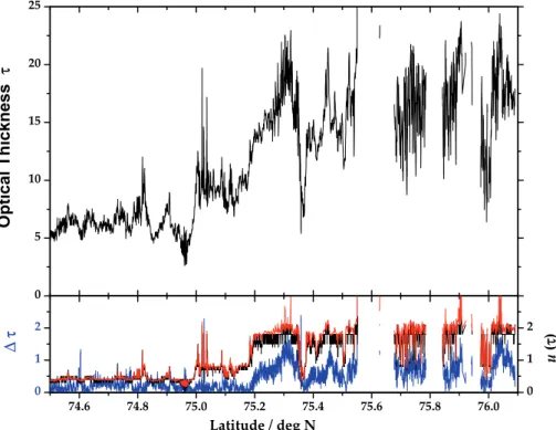
The retrieval results are shown in Fig. 5 for optical thickness τS and in Fig. 6 for

the effective radius r_eS_ff. In the case of optical thickness, the uncertainty (propagated

25

from the reflectance measurement intoτS space) behaves similarly for both retrieval

(8)

AMTD

5, 7753–7781, 2012

E. Bierwirth et al.

Title Page

Tables Figures

◭ ◮

Back Close

Full Screen / Esc

Discussion

P

a

per

|

Dis

cussion

P

a

per

|

Discussion

P

a

per

|

Discussio

n

P

a

per

|

uncertainty, we conclude that either approach can be used to retrieve the optical thick-ness, and the inclusion of additional wavelengths does not provide additional informa-tion.

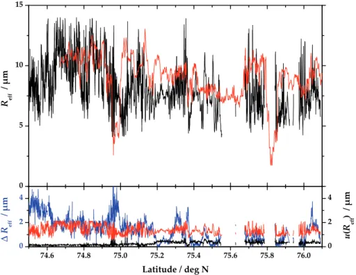
The retrieval ofr_eS_ffis more differentiated. The uncertainties for both approaches differ significantly, with 5WL yielding lower uncertainties (less than 1 µm) than 2WL (1–2 µm).

5

With values between 0 and 4 µm, the di_fference inr_eS_ff between 5WL and 2WL is close to and sometimes exceeds the retrievals’ uncertainties. The additional wavelengths increase the retrieval sensitivity of the effective radius. The FSSP data (shown as red line in Fig. 6) are close to the retrieved value in the southern section of the flight, and deviates more strongly from the retrieval starting at and north of 75◦N. There are two

10

reasons for this: The time difference between in situ observations and remote sensing is smaller in the south, where the aircraft descended from the latter to the former; and south of 75◦N, the in situ observations occurred near the cloud top, while at more northern latitudes the cloud top grew higher and the in situ observations came from a location deeper inside the cloud.

15

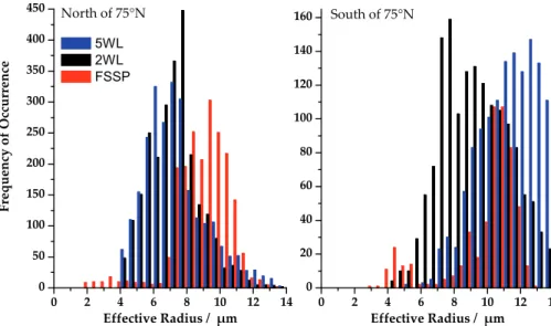
The retrievedr_eS_ff for 2WL and 5WL are compiled in Fig. 7 in form of two histograms, one for the flight section north of 75◦N and one for the section south of 75◦N. It shows that 2WL and 5WL yield similar distributions ofreff for the northern section, and both

deviate equally from the in situ observations that occurred deeper in the cloud. On the other hand, 2WL and 5WL do not agree for the southern flight section, with the

distribu-20

tion from the FSSP observations near cloud top lie between the both. The 5WL retrieval reports a larger amount of large droplets, while 2WL prefers lower values. Judging by the lower retrieval uncertainty of 5WL, the larger values would seem more realistic; however, the deviation from the in situ distribution is beyond the FSSP uncertainty of 1µm. Therefore it is impossible to validate neither 2WL nor 5WL with independent

mea-25

surements, with the time delay between remote sensing and in situ observations being the most likely source of uncertainty.

(9)

AMTD

5, 7753–7781, 2012

E. Bierwirth et al.

Title Page

Tables Figures

◭ ◮

Back Close

Full Screen / Esc

Discussion

P

a

per

|

Dis

cussion

P

a

per

|

Discussion

P

a

per

|

Discussio

n

P

a

per

|

5 Retrieval of cloud properties from hyperspectral radiance

The retrieval of the cloud properties from the hyperspectral radiances uses the same principles as for the spectral radiance. The benefit of the hyperspectral data is that they include o_ff-track pixels, adding another dimension not only to the measured data but also to the look-up tables (viewing angle). However, the AisaEAGLE does not cover

5

wavelengths longer than 1000 nm. Therefore, the effective radius cannot be retrieved for the o_ff-track pixels of the AisaEAGLE because wavelengths shorter than 1000 nm are sensitive to the optical thickness only. In the following, the cloud optical thicknessτE

is retrieved from the 870 nm radiances for each pixel in the field of view of the AisaEA-GLE. For this purpose, the retrieval grid by Nakajima and King (1990) was constrained

10

to a fixed value of the e_ffective radius,r_efix_ff. This value is taken from other measurements on the same flight. As there are several options to choose the constraint of the effective radius, we first tested the sensitivity of the retrieval to the various available values.

5.1 Influence of effective radius

As we have no information about the e_ffective radius in the o_ff-track pixels, we make

15

a basic assumption in the choice of the fixed valuer_efix_ff: the cloud-particle statistics in this stratiform cloud layer is the same inx (flight) and y direction. Our first option for the e_ffective radius is a moving average of the retrieval from the SMART-Albedometer,

r_efix_ff(t)=r_e(1)_ff :=Dr_eS_ff(t−_∆t,t+ ∆t)E. Here, the averaging period ∆t is obtained as fol-lows: First, the width d of the observed strip of cloud is determined from the height

20

h between cloud top and the aircraft (from lidar) and the AisaEAGLE’s field of view (40◦). Then the nadir effective radiir_eS_ff(t) from the SMART-Albedometer are averaged over the time in which the radiance spot on the cloud top covered a distanced that is determined from the aircraft speed as

d=v·t+ 2h·tan(αS/2)

, (2)

(10)

AMTD

5, 7753–7781, 2012

E. Bierwirth et al.

Title Page

Tables Figures

◭ ◮

Back Close

Full Screen / Esc

Discussion

P

a

per

|

Dis

cussion

P

a

per

|

Discussion

P

a

per

|

Discussio

n

P

a

per

|

withαSbeing the viewing angle of the radiance inlet andvthe aircraft speed (ignoring

any cloud motion with the assumption v≪vcloud). The last term in Eq. (2) adds the

radiance field of view behind and in front of the nadir point. Hence, the averaging time interval is [t−∆t,t+ ∆t] with

2_∆t=

d−2h·tanαS 2

.

v. (3)

5

The other options for the choice of the effective radius include instantaneous and aver-aged values from remote sensing (S) or from in situ observations (index i). The com-plete list is this:

1. The moving average in nadir,r_e(1)_ff :=Dr_eS_ff(t−_∆t,t+ ∆t)E;

2. the current e_ffective radius in nadir,r_e(2)_ff(t) :₌r_eS_ff(t);

10

3. the mean effective radius of the entire flight leg,r_e(3)_ff :=Dr_eS_ff(t)E∀t;

4. the value measured by in situ instruments at the same locationx,r_e(4)_ff(t) :₌r_ei_ff(xi= xS(t)), where xi is the aircraft location during the in situ measurements and xS

during the remote-sensing leg;

5. the mean value of all in situ measurements,r_e(5)_ff :=Dr_ei_ff(xi)E∀xi.

15

All five options forr_efix_ff are used as a constraint to derive the optical thickness for all off -track AisaEAGLE pixels. This results in a spread of the optical thicknessτ_ES in the ES pixels of 0.3–0.4 units of optical thickness, which is less than the retrieval uncertainty.

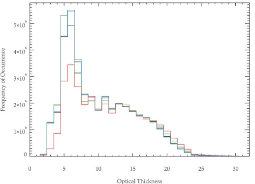
The histograms of the entire field of optical thickness retrieved with the five different constraints of effective radius (Fig. 8) shows that the choice matters only when the

20

(11)

AMTD

5, 7753–7781, 2012

E. Bierwirth et al.

Title Page

Tables Figures

◭ ◮

Back Close

Full Screen / Esc

Discussion

P

a

per

|

Dis

cussion

P

a

per

|

Discussion

P

a

per

|

Discussio

n

P

a

per

|

those low optical thicknesses. This is because of the large time delay between remote sensing and in situ observations. Thin cloud parts are more likely to be changed by weak turbulence than thick stretches of cloud, rendering the local properties detected in situ less representative for the remote sensing at the same location but one hour earlier. We conclude thatr_e(4)_ff is a poor choice, while the other options yield very similar

5

results in the retrieval of the optical thickness.

5.2 Influence of atmospheric profile

The variation of the vertical structure of the atmosphere along the flight track has been recorded by a series of drop sondes. The major change occurred in the height of the cloud top, which increased from 200 m at the southern end of the flight track to 700 m at

10

the northern end. In order to illustrate the potential influence of the atmospheric profile, the look-up tables for the 2WL retrieval were computed for four drop sonde profiles. Between one drop sonde and the next (time interval: 15 min), two sets ofτES differ by

up to 0.2 (0.4 in peaks). The difference is greater when a more distant drop sonde is used; the two retrievals that assume the first and the last drop sonde, respectively,

15

differ by up to one unit of optical thickness. In the following, however, we interpolate between look-up tables created for the different drop sondes in order to mitigate this source of uncertainty.

5.3 Retrieval results

The hyperspectral data from the AisaEAGLE produce a map of the retrieved cloud

20

optical thickness. An example is shown in Fig. 10. This map has been drawn such that the aircraft nadir (marked with the red line) is always in the centre. The wavy edge of the map represents the rolling of the aircraft in flight. The ES pixels that are observed by the SMART-Albedometer radiance surround the nadir point and are delineated by the blue lines.

(12)

AMTD

5, 7753–7781, 2012

E. Bierwirth et al.

Title Page

Tables Figures

◭ ◮

Back Close

Full Screen / Esc

Discussion

P

a

per

|

Dis

cussion

P

a

per

|

Discussion

P

a

per

|

Discussio

n

P

a

per

|

The following statistics of the cloud properties for 17 May are based on the retrieval that uses the current effective radiusr_e(2)_ff(t) from the SMART-Albedometer. The look-up tables were calculated for a range of values of solar zenith angle, cloud-top height, and meteorological profiles, and were then interpolated to the current conditions of each measurement point. The resulting look-up table contained radiances only as a function

5

of viewing angle and cloud optical thickness. The viewing angle is fixed for each pixel of the hyperspectral camera, and modified by the aircraft roll angle. So for each pixel, the radiance is a function ofτ, and the radiance measured by this pixel yields the retrieved

τvalue at this point. On the flight on 17 May, a total of 4×107values were retrieved; see the histogram in Fig. 11. The histograms for the entire field of view and for the ES pixels

10

do not differ significantly, which justifies the assumption that the cloud statistics are the same in flight direction and across (on the scale of the field of view). It can roughly be compared to the nadir values retrieved from the SMART-Albedometer radiance: While the AisaEAGLE has about 20 times more data points, the shape of the distribution is the same as for the nadir optical thickness of the SMART-Albedometer, with the exception

15

of the bins forτ=6–10 that are more pronounced. Only the ES pixels can be directly compared to the simultaneous retrieval by the SMART-Albedometer in nadir (Fig. 12). As these mostly agree within the retrieval uncertainty, the di_fferences in the histogram have to originate in slight off-track deviations in the horizontal distribution of the optical thickness, which nadir observations alone would not observe.

20

6 Conclusions

Both a two-wavelength (2WL) and a five-wavelength (5WL) approach have been ap-plied to retrieve the cloud optical thickness and effective radius from the nadir radiances of the SMART-Albedometer. While the two approaches agree within uncertainty for the optical thickness, they differ in respect to effective radius: 5WL seems to be more

sen-25

sitive to larger droplets (more than 10 µm radius) than 2WL. However, even with com-prehensive instrumentation during the SoRPIC campaign that includes state-of-the-art

(13)

AMTD

5, 7753–7781, 2012

E. Bierwirth et al.

Title Page

Tables Figures

◭ ◮

Back Close

Full Screen / Esc

Discussion

P

a

per

|

Dis

cussion

P

a

per

|

Discussion

P

a

per

|

Discussio

n

P

a

per

|

remote sensing and in situ instrumentation, it is impossible to give a definite answer to the question which of the two methods yields better results. The fundamental limitation is the time delay which cannot be avoided when remote sensing and in situ observa-tions are performed on the same platform, but also the vertical position within the cloud. Only with simultaneous collocated measurements above and inside the cloud (with two

5

aircraft) can this limitation be overcome and can closure between the different methods be attempted.

Hyperspectral imaging was used to retrieve the cloud optical thickness in a 40◦field of view across the flight track. This extends the application of the hyperspectral camera AisaEAGLE to airborne cloud research, and shows the potential of this rapidly

devel-10

oping technology to this purpose. We found that the distribution of the cloud optical thickness derived from the hyperspectral data are not entirely equal to those derived from the nadir radiance. Hyperspectral observations are therefore a tool to improve cloud statistics in remote sensing.

With our current instrumentation, the hyperspectral retrieval is limited to the cloud

15

optical thickness, because the AisaEAGLE does not cover the wavelengths required for a retrieval of the effective radius. However, compatible hyperspectral imagers for those wavelengths already exist and could be successfully applied to retrieve the effective radius additionally.

Acknowledgements. The authors thank the Alfred Wegener Institute for Polar and Marine Re-20

(14)

AMTD

5, 7753–7781, 2012

E. Bierwirth et al.

Title Page

Tables Figures

◭ ◮

Back Close

Full Screen / Esc

Discussion

P

a

per

|

Dis

cussion

P

a

per

|

Discussion

P

a

per

|

Discussio

n

P

a

per

|

References

Barker, H. W., Jerg, M. P., Wehr, T., Kato, S., Donovan, D. P., and Hogan, R. J.: A 3-D cloud construction algorithm for the EarthCARE satellite mission, Q. J. Roy. Meteor. Soc., 137, 1042–1058, 2011. 7755

Bierwirth, E., Wendisch, M., Ehrlich, A., Heese, B., Tesche, M., Althausen, D., Schladitz, A., 5

M ¨uller, D., Otto, S., Trautmann, T., Dinter, T., von Hoyningen-Huehne, W., and Kahn, R.: Spectral surface albedo over Morocco and its impact on radiative forcing of Saharan dust, Tellus B, 61, 252–269, 2009. 7756

Brest, C. L., Rossow, W. B., and Roiter, M. D.: Update of Radiance Calibrations for ISCC P., J. Atmos. Ocean. Technol., 14, 1091–1109, 1997. 7755

10

Coddington, O. M., Pilewskie, P., Redemann, J., Platnick, S., Russell, P. B., Schmidt, K. S., Gore, W. J., Livingston, J., Wind, G., and Vukicevic, T.: Examining the impact of overlying aerosols on the retrieval of cloud optical properties from passive remote sensing, J. Geophys. Res., 115, D10211, doi:10.1029/2009JD012829, 2010. 7759

Crowther, B.: The Design, Construction, and Calibration of a Spectral Diffuse/Global Irradiance 15

Meter, Ph. D. thesis, University of Arizona, Tucson, USA, 1997. 7756

Curry, J. A., Rossow, W. B., Randall, D., and Schramm, J. M.: Overview of Arctic cloud and radiation characteristics, J. Climate, 9, 1731–1764, 1996. 7754

de Boer, G., Hashino, T., and Tripoli, G. J.: Ice nucleation through immersion freezing in mixed-phase stratiform clouds: Theory and numerical simulations, Atmos. Res., 96, 315–324, 2010. 20

7754

Dietzsch, F.: Charakaterisierung der synoptischen Situation w ¨ahrend der Kampagne SORPIC April/Mai 2010, B. S. Thesis, University of Leipzig, Germany, 2010. 7758

Dye, J. E. and Baumgardner, D.: Evaluation of the forward scattering spectrometer probe. Part I: electronic and optical studies, J. Atmos. Ocean. Tech., 1, 329–344, 1984. 7757

25

Ehrlich, A., Wendisch, M., Bierwirth, E., Herber, A., and Schwarzenb ¨ock, A.: Ice crystal shape effects on solar radiative properties of arctic mixed-phase clouds – dependence on micro-physical properties, Atmos. Res., 88, 266–276, 2008. 7754

Ehrlich, A., Bierwirth, E., Wendisch, M., Herber, A., and Gayet, J.-F.: Airborne hyperspectral observations of surface and cloud directional reflectivity using a commercial digital camera, 30

Atmos. Chem. Phys., 12, 3493–3510, doi:10.5194/acp-12-3493-2012, 2012. 7757

(15)

AMTD

5, 7753–7781, 2012

E. Bierwirth et al.

Title Page

Tables Figures

◭ ◮

Back Close

Full Screen / Esc

Discussion

P

a

per

|

Dis

cussion

P

a

per

|

Discussion

P

a

per

|

Discussio

n

P

a

per

|

Formenti, P. and Wendisch, M.: Combining upcoming satellite missions and aircraft activities, B. Am. Meteorol. Soc., 89, 385–388, 2008. 7755

Gayet, J. F., Cr ´epel, O., Fournol, J. F., and Oshchepkov, S.: A new airborne polar Nephelome-ter for the measurements of optical and microphysical cloud properties. Part I: Theoretical design, Ann. Geophys., 15, 451–459, doi:10.1007/s00585-997-0451-1, 1997. 7757

5

Herber, A., Dethloff, K., Haas, C., Steinhage, D., Strapp, J. W., Bottenheim, J., McElroy, T., and Yamanouchi, T.: POLAR 5 – a new research aircraft for improved access to the Arctic, in: Extended Abstracts of the First International Symposium on the Arctic Research (ISAR–1), Miraikan, Japan, 4–6 November 2008, 54–57, 2008. 7755

Korolev, A. and Isaac, G. A.: Relative humidity in liquid, mixed-phase, and ice clouds, J. Atmos. 10

Sci., 63, 2865–2880, doi:10.1175/JAS3784.1, 2006. 7754

Krijger, J. M., Tol, P., Istomina, L. G., Schlundt, C., Schrijver, H., and Aben, I.: Improved identifi-cation of clouds and ice/snow covered surfaces in SCIAMACHY observations, Atmos. Meas. Tech., 4, 2213–2224, doi:10.5194/amt-4-2213-2011, 2011. 7754

Lawson, R. P., Korolev, A. V., Cober, S. G., Huang, T., Strapp, J. W., and Isaac, G. A.: Improved 15

measurements of the drop size distribution of a freezing drizzle event, Atmos. Res., 47–48, 181–191, 1998. 7757

Marshak, A., Platnick, S., V ´arnai, T., Wen, G., and Cahalan, R. F.: Impact of three-dimensional radiative effects on satellite retrievals of cloud droplet sizes, J. Geophys. Res., 111, D09207, doi:10.1029/2005JD006686, 2006. 7755

20

Mayer, B. and Kylling, A.: Technical note: the libRadtran software package for radiative trans-fer calculations – description and examples of use, Atmos. Chem. Phys., 5, 1855–1877, doi:10.5194/acp-5-1855-2005, 2005. 7758

McBean, G., Alekseev, G., Chen, D., Forland, E., Fyfe, J., Groisman, P. Y., King, R., Melling, H., Vose, R., and Whitfield, P. H.: Arctic Climate: Past and Present, in Arctic Climate Impact 25

Assessment, edited by: Symon, C., Arris, L., and Heal, B., 21–60, Cambridge University Press, New York, NY, 2005. 7754

Nakajima, T. and King, M.: Determination of the optical thickness and e_ffective particle radius of clouds from reflected solar radiation measurements. Part I: theory, J. Atmos. Sci., 47, 1878–1893, 1990. 7759, 7761

30

(16)

AMTD

5, 7753–7781, 2012

E. Bierwirth et al.

Title Page

Tables Figures

◭ ◮

Back Close

Full Screen / Esc

Discussion

P

a

per

|

Dis

cussion

P

a

per

|

Discussion

P

a

per

|

Discussio

n

P

a

per

|

Pietsch, A.: Analyse der Messgenauigkeit von Temperatur- und Feuchteprofilen aus Flugzeug-, Radiosonden- und Dropsondenmessungen und Vergleich mit Simulationen des ECMWF-Modells f ¨ur Fallbeispiele der SORPIC Messkampagne, B. S. Thesis, University of Leipzig, Germany, 2011.

Seifert, P., Ansmann, A., Mattis, I., Wandinger, U., Tesche, M., Engelmann, R., M ¨uller, D., 5

P ´erez, C., and Haustein, K.: Saharan dust and heterogeneous ice formation: Eleven years of cloud observations at a Central European EARLINET site, J. Geophys. Res., 115, D20201, doi:10.1029/2009JD013222, 2010. 7754

Shupe, M. D. and Intrieri, J. M.: Cloud radiative forcing of the arctic surface: the influence of cloud properties, surface albedo, and solar zenith angle, J. Climate., 17, 616–628, 2004. 10

7755

Stachlewska, I. S., Neuber, R., Lampert, A., Ritter, C., and Wehrle, G.: AMALi – the air-borne mobile aerosol lidar for arctic research, Atmos. Chem. Phys., 10, 2947–2963, doi:10.5194/acp-10-2947-2010, 2010. 7756

Walsh, J. E., Overland, J. E., Groisman, P. Y., and Rudolf, B.: Ongoing climate change in the 15

Arctic, AMBIO, 40, 6–16, doi:10.1007/s13280-011-0211-z, 2011. 7754

Wendisch, M. and Brenguier, J.-L. (Eds.): Airborne Measurements for Environmental Research: Methods and Instruments, Wiley-VCH Verlag GmbH & Co. KGaA, Weinheim, Germany, ISBN: 978-3-527-40996-9, in press, 2013. 7756

Wendisch, M., M ¨uller, D., Schell, D., and Heintzenberg, J.: An airborne spectral albedometer 20

with active horizontal stabilization, J. Atmos. Ocean. Tech., 18, 1856–1866, 2001. 7757 Wu, D. L. and Lee, J. N.: Arctic low cloud changes as observed by MISR and CALIOP:

implica-tion for the enhanced autumnal warming and sea ice loss, J. Geophys. Res., 117, D07107, doi:10.1029/2011JD017050, 2012. 7754

(17)

AMTD

5, 7753–7781, 2012

E. Bierwirth et al.

Title Page

Tables Figures

◭ ◮

Back Close

Full Screen / Esc

Discussion

P

a

per

|

Dis

cussion

P

a

per

|

Discussion

P

a

per

|

Discussio

n

P

a

per

|

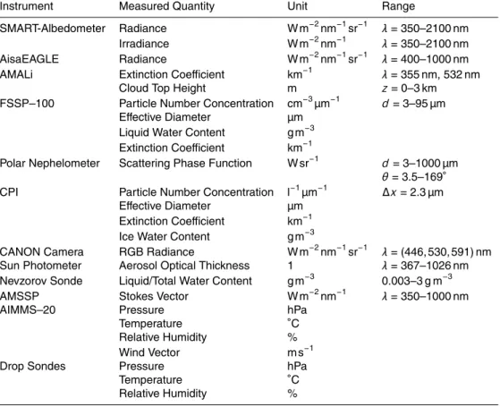
Table 1.Instrumentation during SoRPIC. Acronyms: AMALi, FSSP (Forward Scattering Spec-trometer Probe), CPI (Cloud Particle Imager), AMSSP (Airborne Multi Spectral Sunphoto- and Polarimeter), AIMMS (Advanced Airborne MeasureMent Solutions).

Instrument Measured Quantity Unit Range

SMART-Albedometer Radiance W m−2nm−1sr−1 λ=350–2100 nm

Irradiance W m−2nm−1 λ=350–2100 nm

AisaEAGLE Radiance W m−2nm−1sr−1 λ=400–1000 nm

AMALi Extinction Coefficient km−1 λ=355 nm, 532 nm

Cloud Top Height m z=0–3 km

FSSP–100 Particle Number Concentration cm−3µm−1 d=3–95 µm

Effective Diameter µm

Liquid Water Content g m−3

Extinction Coefficient km−1

Polar Nephelometer Scattering Phase Function W sr−1 d=3–1000 µm

θ=3.5–169◦

CPI Particle Number Concentration l−1µm−1 ∆x=2.3 µm

Effective Diameter µm

Extinction Coefficient km−1

Ice Water Content g m−3

CANON Camera RGB Radiance W m−2nm−1sr−1 λ=(446, 530, 591) nm

Sun Photometer Aerosol Optical Thickness 1 λ=367–1026 nm

Nevzorov Sonde Liquid/Total Water Content g m−3 0.003–3 g m−3

AMSSP Stokes Vector W m−2nm−1 λ=350–1000 nm

AIMMS–20 Pressure hPa

Temperature ◦C

Relative Humidity %

Wind Vector m s−1

Drop Sondes Pressure hPa

Temperature ◦C

(18)

AMTD

5, 7753–7781, 2012

E. Bierwirth et al.

Title Page

Tables Figures

◭ ◮

Back Close

Full Screen / Esc

Discussion

P

a

per

|

Dis

cussion

P

a

per

|

Discussion

P

a

per

|

Discussio

n

P

a

per

|

Fig. 1.Viewing geometry for radiances from the Polar-5 aircraft with the hyperspectral cam-era AisaEAGLE (black) and the SMART-Albedometer (blue). Typical dimensions in this study: distance aircraft–cloudh=2600 m, aircraft speedv=70 m s−1, width of one AisaEAGLE pixel y_E=3.5 m, length x_E=y_E+v·t_E=4.2 m with the exposure timet_E=10 ms, width of instan-taneous SMART-Albedometer field of viewy_S=68 m, length due to exposure time t_S=0.5 s: x_S=y_S+v·t_S=103 m.

(19)

AMTD

5, 7753–7781, 2012

E. Bierwirth et al.

Title Page

Tables Figures

◭ ◮

Back Close

Full Screen / Esc

Discussion

P

a

per

|

Dis

cussion

P

a

per

|

Discussion

P

a

per

|

Discussio

n

P

a

per

|

(20)

AMTD

5, 7753–7781, 2012

E. Bierwirth et al.

Title Page

Tables Figures

◭ ◮

Back Close

Full Screen / Esc

Discussion

P

a

per

|

Dis

cussion

P

a

per

|

Discussion

P

a

per

|

Discussio

n

P

a

per

|

Fig. 3.ECMWF analysis chart (925 hPa, 12:00 UTC) and SoRPIC flight track on 17 May 2010, from Longyearbyen (LY) to 50 km east of Bjørnøya (B) and back. Dropsondes were launched at the D symbols. The contours are the geopotential height in m (green) and the equivalent potential temperature in K (blue).

(21)

AMTD

5, 7753–7781, 2012

E. Bierwirth et al.

Title Page

Tables Figures

◭ ◮

Back Close

Full Screen / Esc

Discussion

P

a

per

|

Dis

cussion

P

a

per

|

Discussion

P

a

per

|

Discussio

n

P

a

per

|

P

ap

er

|

Disussion

P

ap

er

|

Disussion

P

ap

er

|

Disussion

P

ap

er

Fig. 4.Dropsonde profiles (red: temperature, blue: relative humidity) and lidar cloud-top altitude (black) for 17 March 2010. Each drop-sonde profile is marked with one dashed and two dotted lines; the dashed lines are placed at the times of launch, and also represent a temperature of 12◦C and 100 % RH. The central dotted lines show 6◦C and 50 %, the left dotted lines show 0◦C and 0 %. The green line represents the flight altitude during the in situ observations.

(22)

AMTD

5, 7753–7781, 2012

E. Bierwirth et al.

Title Page

Tables Figures

◭ ◮

Back Close

Full Screen / Esc

Discussion

P

a

per

|

Dis

cussion

P

a

per

|

Discussion

P

a

per

|

Discussio

n

P

a

per

|

Fig. 5. Top panel: cloud optical thickness τ in aircraft nadir, retrieved from the SMART-Albedometer reflectance by 2WL. Bottom panel: absolute difference ∆τ between τ retrieved by 2WL and 5WL (blue); propagated uncertaintyu(τ) in 5WL (black) and 2WL (red).

(23)

AMTD

5, 7753–7781, 2012

E. Bierwirth et al.

Title Page

Tables Figures

◭ ◮

Back Close

Full Screen / Esc

Discussion

P

a

per

|

Dis

cussion

P

a

per

|

Discussion

P

a

per

|

Discussio

n

P

a

per

|

(24)

AMTD

5, 7753–7781, 2012

E. Bierwirth et al.

Title Page

Tables Figures

◭ ◮

Back Close

Full Screen / Esc

Discussion

P

a

per

|

Dis

cussion

P

a

per

|

Discussion

P

a

per

|

Discussio

n

P

a

per

|

Fig. 7. Histograms showing the effective radius, retrieved from the SMART-Albedometer re-flectance by 5WL (blue) and 2WL (black) and as observed by the FSSP (red) at the same latitude, but one hour later. Left: for the flight section north of 75◦N. Right: South of 75◦N.

(25)

AMTD

5, 7753–7781, 2012

E. Bierwirth et al.

Title Page Abstract Introduction Conclusions References Tables Figures ◭ ◮ ◭ ◮ Back Close

Full Screen / Esc

0 2 4 6 8 10 12 14

0 50 100 150 200 250 300 350 400 450

South of 75°N

5W L 2W L FSSP F r eq u en c y o f O c c u r r en c e

Effective Radius / µm

0 2 4 6 8 10 12 14

0 20 40 60 80 100 120 140 160 North of 75°N

Effective Radius / µm

(26)

AMTD

5, 7753–7781, 2012

E. Bierwirth et al.

Title Page

Tables Figures

◭ ◮

Back Close

Full Screen / Esc

Discussion

P

a

per

|

Dis

cussion

P

a

per

|

Discussion

P

a

per

|

Discussio

n

P

a

per

|

P

ap

er

|

Disussion

P

ap

er

|

Disussion

P

ap

er

|

Disussion

P

ap

er

Fig. 9.Influence of the atmospheric profile used in the creation of the look-up tables.

(27)

AMTD

5, 7753–7781, 2012

E. Bierwirth et al.

Title Page

Tables Figures

◭ ◮

Back Close

Full Screen / Esc

Discussion

P

a

per

|

Dis

cussion

P

a

per

|

Discussion

P

a

per

|

Discussio

n

P

a

per

|

P

ap

er

|

Disussion

P

ap

er

|

Disussion

P

ap

er

|

Disussion

P

ap

er

Fig. 10.Map of the cloud optical thickness, retrieved from hyperspectral radiance measure-ments by the AisaEAGLE on 17 May 2010 at 10:14 UTC. The red curve shows true nadir, the blue lines delineate the field of view of the SMART-Albedometer radiance.

(28)

AMTD

5, 7753–7781, 2012

E. Bierwirth et al.

Title Page

Tables Figures

◭ ◮

Back Close

Full Screen / Esc

Discussion

P

a

per

|

Dis

cussion

P

a

per

|

Discussion

P

a

per

|

Discussio

n

P

a

per

|

Fig. 11.Histogram of the cloud optical thickness retrieved from the hyperspectral radiances in all pixels (red) and in the nadir (ES) pixels (gray); and from the SMART-Albedometer nadir radiances (5WL algorithm in blue, 2WL in black).

(29)

AMTD

5, 7753–7781, 2012

E. Bierwirth et al.

Title Page

Tables Figures

◭ ◮

Back Close

Full Screen / Esc

Discussion

P

a

per

|

Dis

cussion

P

a

per

|

Discussion

P

a

per

|

Discussio

n

P

a

per

|