http://dx.doi.org/10.20852/ntmsci.2016115852
On the solution of differential equation system
characterizing curve pair of constant Breadth by the
Lucas collocation approximation
Muhammed Cetin, Huseyin Kocayigit and Mehmet Sezer
Department of Mathematics, Celal Bayar University, Manisa, Turkey
Received: 17 August 2015, Revised: 18 August 2015, Accepted: 30 September 2015 Published online: 10 February 2016.
Abstract: In this study, for solving linear differential equation system characterizing curve pair of constant breadth according to Bishop frame in Euclidean 3-space, a new collocation method based on Lucas polynomials is introduced and hence the curve pair of constant breadth is determined. Furthermore, an error analysis based on residual error function is given for the method. To demonstrate the accuracy and effciency of the method, an example is given with the help of computer programmes Maple and Matlab.
Keywords: Curves pair of constant breadth, Bishop frame, Lucas polynomial and series, collocation points, system of differential equations.
1 Introduction
The curves of constant breadth were introduced by Euler in 1778 [1]. He investigated these curves in the plane. After him, many mathematicians were interested in these curves [2-11]. Ma˘gden and K¨ose studied the curves of constant breadth inE4-space in [12]. Then, the concepts related to constant breadth space curve were extended toEn-space in [13]. Sezer established the differential equations characterizing curves of constant breadth and gave a criterion for these curves in [14]. Furthermore, ¨Onder et al gave the differential equations characterizing the constant breadth timelike and spacelike curves in Minkowski 3-spaceE13in [15]. Also Kocayi˘git and ¨Onder showed that inE13spacelike and timelike curves of constant breadth are related to normal curves, spherical curves and helices in some special cases [16]. In [17], Kocayi˘git and C¸ etin investigated the constant breadth space curves according to Bishop frame in Euclidean 3-space. Then, C¸ etin et al used a collocation method based on Taylor polynomials for the approximate solutions of the linear differential equation system characterizing constant breadth curves in Euclidean 3-spaceE3. So, curve pair of constant breadth is determined [18].
In [19], the collocation method based on Taylor polynomials was given by Sezer et al in order to find the approximate solutions of high-order systems of linear differential equations with variable coeffcients. In addition, C¸ etin et al presented an approximation method based on Lucas polynomials for the solution of the system of high-order linear differential equations with variable coeffcients under the mixed conditions [20].
constant breadth according to Bishop frame in Euclidean 3-space by using Lucas collocation method. Then, an example is given to demonstrate the effciency of the method.
2 Preliminaries
Firstly, we give some basic concepts on classical differential geometry of space curves. Letα(s)be an unit speed space curve and let{−→T(s),−→N(s),−→B(s)}be Frenet frame of this curve. The elements of the frame−→T,−→N and−→B are called the unit tangent vector, the unit principal normal vector and the unit binormal vector of the curve, respectively. Moreover,
κ(s)andτ(s)are called curvature and torsion of the curveα, respectively. The Frenet formulae are also well known as
− →T′ − →N′ − →B′
=
0 κ 0
−κ 0 τ
0 −τ0
− →T − →N − →B
where⟨−→T,−→T⟩=⟨−→N,−→N⟩=⟨−→B,−→B⟩=1 and⟨−→T,−→N⟩=⟨−→N,−→B⟩=⟨−→T,−→B⟩=0. The parallel transport frame is an alternative approach to defining a moving frame that is well-defined even when the curve has vanishing second derivative. We can parallel transport an orthonormal frame along a curve simply by paralel transporting each component of the frame [21].
Its mathematical properties derive from the observation that, while−→T(s)for a given curve model is unique, we may choose any convenient arbitrary basis(−N→1(s),−N→2(s)
)
for the remainder of the frame, so long as it is in the normal plane
perpendicular to−→T(s)at each point. If the derivatives of(−N→1(s),−N→2(s)
)
depend only on−→T(s)and not each other, we can make −N→1(s) and−N→2(s) vary smoothly throughout the path regardless of the curvature. We may therefore choose the
alternative frame equations
− →T′ −→ N1′
−→ N2′
=
0 k1k2
−k1 0 0
−k2 0 0
− →T −→ N1
−→ N2
(1)
where⟨−→T,−→T⟩=⟨−N→1,−N→1
⟩
=⟨−N→2,−N→2
⟩
=1 and⟨−→T,−N→1
⟩
=⟨−N→1,−N→2
⟩
=⟨−→T,−N→2
⟩
=0 [22, 23].
One can show that [22]
κ(s) =√k2
1+k22,θ(s) =arctan
( k2
k1 )
,τ(s) =dθds(s)
k1=κcos(θ), k2=κsin(θ),
and
− →T =−→T
,−N→1(s) =−→Ncos(θ)−−→Bsin(θ),−N→2(s) =−→Nsin(θ) +−→Bcos(θ)
It is well-known that the curvatureκ(s)of the curve (C) is defined by
lim ∆s→0
∆ϕ ∆s =
dϕ ds =κ(s)
whereϕis the angle between the tangent−→T of the curveα and a given fixed direction at the pointα(s).
3 Lucas Collocation Method for Linear Differential Equation System with Variable
Coefficients in Normal Form
C¸ etin et al presented a collocation method based on Lucas polynomials to find the approximate solutions of high-order linear differential equation systems with variable coefficients in [20]. In this section, by means of the matrix relations between Lucas polynomials and their derivatives, we give a new method for solving the linear differential equation system in normal form as
L[yi(x)] =yi′(x)− m
∑
j=1pi,j(x)yj(x) =gi(x) (i=1,2, ...,m) (0≤a≤x≤b) (2)
under the initial conditions
yi(a) =ci (3)
whereyi(x) (i=1,2, ...,m) are unknown functions, pi,j(x)and gi(x) are the known continuous functions defined on interval[a,b], andci (i=1,2, ...,m)are the real constants. In this part, by means of Lucas collocation method with the help of the residual error function [24-27], we obtain the approximate solutions of the system (2) expressed in the truncated Lucas series
yi,N,M(x) =yi,N(x) +ei,N,M(x) (i=1,2, ...,m) where
yi(x)∼=yi,N(x) = N
∑
n=0ai,nLn(x) (4)
is the Lucas polynomial solutions and
ei,N,M(x) = M
∑
n=0a∗i,nLn(x) (M>N)
is the estimated error function obtained with the help of the residual error function. Hereai,nanda∗i,nare the unknown Lucas coefficients andLn(x) (n=0,1,2, ...,N)are the Lucas polynomials defined by [28,29],
L0(x) =2;Ln(x) =
[[n/2]]
∑
k=0n n−k
( n−k
k )
xn−2k, (n≥1), [[n/2]]=
{
n/2 , neven
(n−1)/2 , nodd ;
In order to find the solutions of the system (2) under the initial conditions (3), we can use the collocation points defined by
xk=a+
b−a
On the other hand, we can write the approximate solutionsyi,N(x)given by Eq.(4) in the matrix form
yi,N(x) =L(x)Ai, (i=1,2, ...,m) (6)
where
L(x) =[L0(x)L1(x)L2(x)··· LN(x) ]
and
Ai=[ai,0ai,1ai,2···ai,N ]T
.
Here, the Lucas polynomialsLn(x)can be written in the matrix form as
L(x) =X(x)DT (7)
such that
X(x) =[1 x x2 ··· xN ]
and ifNis odd,
D=
2 0 0 0 0 ··· 0
0 1 1 ( 1 0 )
0 0 0 ··· 0
2 1 ( 1 1 ) 0 2 2 ( 2 0 )
0 0 ··· 0
0 3 2 ( 2 1 ) 0 3 3 ( 3 0 )
0 ··· 0
4 2 ( 2 2 ) 0 4 3 ( 3 1 ) 0 4 4 ( 4 0 ) ··· 0 . . . . . . . . . . . . . . . . . . . . .
n−1 (n−1)/2
(
(n−1)/2
(n−1)/2
)
0 n−1 (n+1)/2
(
(n+1)/2
(n−3)/2
)
0 n−1 (n+3)/2
(
(n+3)/2
(n−5)/2
)
0
0 n
(n+1)/2
(
(n+1)/2
(n−1)/2
)
0 n
(n+3)/2
(
(n+3)/2
(n−3)/2
)
0 ··· n n ( n 0 ) .
IfNis even,
D=
2 0 0 0 0 ··· 0
0 1 1 ( 1 0 )
0 0 0 ··· 0
2 1 ( 1 1 ) 0 2 2 ( 2 0 )
0 0 ··· 0
0 3 2 ( 2 1 ) 0 3 3 ( 3 0 )
0 ··· 0
4 2 ( 2 2 ) 0 4 3 ( 3 1 ) 0 4 4 ( 4 0 ) ··· 0 . . . . . . . . . . . . . . . . . . . . . 0 n−1
n/2
( n/2
(n−2)/2
)
0 n−1 (n+2)/2
(
(n+2)/2
(n−4/2
)
0 ··· 0
n n/2
( n/2
n/2
)
0 n
(n+2)/2
(
(n+2)/2
(n−2)/2
)
0 n
(n+4)/2
(
(n+4)/2
(n−4)/2
From Eq.(6) and Eq.(7), we obtain the matrix relation
yi,N(x) =X(x)DTAi, (i=1,2, ...,m). (8)
Therefore, the matricesyi,N(x),(i=1,2, ...,m)can be expressed as
Y(x) =X(x)DA. (9)
where
Y(x) =
y1,N(x)
y2,N(x) .. .
ym,N(x) , X(
x) =
X(x) 0 ··· 0 0 X(x)··· 0 ..
. ... . .. ... 0 0 ··· X(x)
, D=
DT 0 ··· 0 0 DT ··· 0
..
. ... . .. ... 0 0 ··· DT
,A= A1 A2 .. . Am .
Also, the relation between the matrix X(x)and its derivative X′(x)is
X′(x) =X(x)B (10)
where B=
0 1 0 ··· 0 0 0 2 ··· 0 ..
. ... ... . .. ... 0 0 0 ··· N
0 0 0 ··· 0 .
By using the relations (8) and (10), we obtain the following matrix relation
y′i,N(x) =X(x)BDTAi. (i=1,2, ...,m) (11)
Hence, we can write the matrix relations as follow
Y′(x) =X(x)BDA (12)
where
Y′(x) =
y′1,N(x)
y′2,N(x)
.. .
y′m,N(x)
, B=
B 0 ··· 0 0 B ··· 0
..
. ... . .. ... 0 0 ··· B
4 Method for solution
We can write the system (2) in the matrix form
Y′(x) =P(x)Y(x) +G(x) (13)
where
P(x) =
p1,1(x) p1,2(x)··· p1,m(x)
p2,1(x) p2,1(x)··· p2,1(x)
..
. ... . .. ...
pm,1(x)pm,2(x)··· pm,m(x) , G(
x) =
g1(x)
g2(x)
.. .
gm(x) .
By using the collocation points given by (5) into Eq.(13), we obtain the system of matrix equations
Y′(xk) =P(xk)Y(xk) +G(xk),(k=0,1, ...,N). Briefly, the fundamental matrix equation is
Y′=PY+G (14)
where P=
P(x0) 0 ··· 0
0 P(x1)··· 0
..
. ... . .. ... 0 0 ··· P(xN)
, Y=
Y(x0)
Y(x1)
.. . Y(xN)
, Y
′=
Y′(x0)
Y′(x1)
.. . Y′(xN)
, G=
G(x0)
G(x1)
.. . G(xN)
.
From the relations (9) and (12) and the collocation points given by (5), we obtain
Y(xk) =X(xk)DA and Y′(xk) =X(xk)BDA,(k=0,1, ...,N) or briefly
Y=XDA and Y′=XBDA (15) where X=
X(x0)
X(x1)
.. . X(xN)
, X(
xk) =
X(xk) 0 ··· 0 0 X(xk)··· 0
..
. ... . .. ... 0 0 ··· X(xk)
.
By substituting the relations given by (15) into Eq.(14), we gain the fundamental matrix equation as
{
XBD−PXD}A=G. (16)
In Eq.(16) the full dimensions of the matrices P, X, B, D, A and G arem(N+1)×m(N+1),m(N+1)×m(N+1),
m(N+1)×m(N+1),m(N+1)×m(N+1),m(N+1)×1 andm(N+1)×1, respectively.
The fundamental matrix equation (16) corresponding to Eq.(2) can be written in the form
This is a linear system ofm(N+1)algebraic equations inm(N+1)the unknown Lucas coefficients such that
W=XBD−PXD= [wp,q], p,q=1,2, ...,m(N+1).
By using the conditions given by (5) and the relations (9), the matrix form for the conditions is obtained as
X(a)DA=C (18)
where
C=[c1c2··· cm ]T
.
Hence, the fundamental matrix form for conditions is
UA=C or [U; C] (19)
such that
U=X(a)D.
Consequently, we obtain the Lucas polynomial solution of the system (2) under the initial conditions (3) by replacing the row matrices (19) by last rows of the matrix (17). Then, we obtain the new augmented matrix
e
WA=G ore [W;e Ge]. (20)
If rankWe =rank[W;e Ge]=N+1, then we can write
A=(We)−
1
e
G. (21)
By solving this linear system, the unknown Lucas coefficients matrix A is determined andai,0,ai,1, ...,ai,N(i=1,2, ...,m) are substituted in Eq.(4). Thus, we find the Lucas polynomial solutions
yi,N(x) = N
∑
n=0ai,nLn(x), (i=1,2, ...,m).
5 Residual correction and error estimation
In this section, we give an error estimation for the Lucas polynomial solutions (4) with the residual error function [24-27]. In addition, we develop the Lucas polynomial solutions (4) by means of the residual error function. Firstly, we can define the residual error function for the Lucas collocation method as
Ri,N(x) =L[yi,N(x)]−gi(x), (i=1,2, ...,m). (22)
Here,yi,N(x)represent the Lucas polynomial solutions given by (4) of the problem (2) and (3). Hence,yj,N(x)satisfies the
problem
y′i,N(x)− ∑m
j=1
pi,j(x)yj,N(x) =gi(x) +Ri,N(x), (i=1,2, ...,m)
Also, the error functionei,N(x)can be defined as
ei,N(x) =yi(x)−yi,N(x) (23)
whereyi(x)are the exact solutions of the problem (2) and (3). From Eqs.(2), (3), (22) and (23), we obtain a system of error differential equations
L[ei,N(x)] =L[yi(x)]−L[yi,N(x)] =−Ri,N(x) with the homogeneous initial conditions
ei,N(a) =0,(i=1,2, ...,m), or openly, the error problem can be expressed as
e′i,N(x)− m
∑
j=1
pi,j(x)ej,N(x) =−Ri,N(x), (i=1,2, ...,m)
ei,N(a) =0, (i=1,2, ...,m).
(24)
Here, the nonhomegeneous initial conditions
yi(a) =ciandyi,N(a) =ci are reduced to homogeneous initial conditions
ei,N(a) =0.
The error problem (24) can be solved by using the prosedure given in Section 3-4. Thus, we obtain the approximation
ei,N,M(x) = M
∑
n=0a∗i,nLn(x), (M>N, i=1,2, ...,m)
toei,N(x). Consequently, the corrected Lucas polynomial solutionyi,N,M(x) =yi,N(x) +ei,N,M(x)is obtained by means of the polynomialsyi,N(x)andei,N,M(x). In addition, we construct the error functionei,N(x) =yi(x)−yi,N(x), the estimated error functionei,N,M(x)and the corrected error functionEi,N,M(x) =yi(x)−yi,N,M(x).
6 Illustration
In this section, we give an example. In tables and figures, we calculate the values of the Lucas polynomial solutions
yi,N(x), the corrected Lucas polynomial solutionsyi,N,M(x) =yi,N(x) +ei,N,M(x)and the estimated absolute error function
|ei,N,M(x)|.
Definition 1. A pair of space curves(C)and (C∗)in E3for which the tangents at the corresponding points α(s)and α∗(s∗)are parallel and in opposite directions, and the distance between these points is always constant are called space curve pair of constant breadth [11].
Let(C)and(C∗)be a pair of unit-speed curves in Euclidean 3-space with non-zero Bishop curvatures and let those curves have paralel tangents in opposite directions at the corresponding pointsα(s)andα∗(s∗), repectively. Hence, the position
vector of the curve(C∗)at the pointα∗(s∗)can be written as −→
whereλi(s) (i=1,2,3)are differentiable functions ofswhich is arc lenght of(C). Denote by {−→
T,−N→1,−N→2
}
,k1andk2the
moving Bishop frame, Bishop curvatures along the curve(C), respectively. And denote by{−T→∗,−N→1∗,−N→2∗},k1∗andk∗2the moving Bishop frame, Bishop curvatures along the curve(C∗), respectively.
Theorem 1.The general differential equations system characterizing space curve pair of constant breadth according to
Bishop frame in E3is as follows [17].
dλ1
ds =k1λ2+k2λ3 dλ2
ds =−k1λ1 dλ3
ds =−k2λ1
(26)
where k1and k2are Bishop curvatures defined by
k1=κ(s)cos(θ)and k1=κ(s)sin(θ),(θ= ∫
τ(s)ds).
The position vector of the curve(C∗)at the pointα∗(s∗)in terms ofα′,α′′,α′′′andk1,k2by means of the Bishop formulae
as follows [18].
−→ α∗(s∗) =
(
k1λ3−k2λ2 µ
) − →α′′′+
(
k2′λ2−k1′λ3 µ
) − →α′′+
[ (
k21+k22)(k1λ3−k2λ2)
µ +λ1
] − →α′+−→α
such that
µ=k21 (k
2
k1
)′
.
Example 1.Let us consider the curveα:[0,2π]→E3given by
α(s) =
( cos(s
2 )
,sin(s 2 ) , √ 3s 2 ) .
For the curveαcurvature, torsion and Bishop elements are calculated as
κ=1 4,τ=
√ 3 4 ,θ=
√ 3s
4
k1=
1 4cos (√ 3s 4 )
and k2=
1 4sin (√ 3s 4 ) . (27)
Substituting (27) in (26), we obtain
λ1′=14cos
(√ 3s
4
)
λ2+14sin
(√ 3s
4
)
λ3
λ2′=−14cos
(√ 3s
4
)
λ1
λ3′=−14sin
(√ 3s 4 ) λ1 (28)
We can find the approximate solutions of the problem (28) by using Lucas collocation method above mentioned. We suppose that the initial conditions forλ1(s),λ2(s)andλ3(s)as follows
λ1(0) =1,λ2(0) =4,λ3(0) =2.
The approximate solutionsλ1,3(s),λ2,3(s)andλ3,3(s)by the truncated Lucas series forN=3 are given by
λi,3(s) = 3
∑
n=0The set of the collocation points fora=0,b=2π andN=3 is calculated as {
s0=0,s1=
2π
3 ,s2= 4π
3 ,s3=2π }
.
We can write the fundamental matrix equation of the problem (28) from Eq.(16) as
{
SBD−PSD}A=G.
By using the method in Section 3-4, the approximate solutions of the problem (28) forN=3 are obtaied as
λ1,3=1.0000000000000000278+0.9999999999999994904s+ (0.230862972284423679e−1)s2
−(0.268502435025769032e−1)s3
λ2,3=4.000000000000000318−0.2499999999999998461s−0.153376809980715401s2
+ (0.332975802130747873e−1)s3
λ3,3=2.000000000000000098+ (0.36e−17)s−0.172375652146830871s2+ (0.107444813448467590e−1)s3.
In order to calculate the corrected Lucas polynomial solutions, let us consider the error problem
e′1,3(s)−14cos
(√ 3s
4
)
e2,3(s)−14sin
(√ 3s
4
)
e3,3(s) =−R1,3(s)
e′2,3(s) +14cos
(√ 3s
4
)
e1,3(s) =−R2,3(s)
e′3,3(s) +14sin
(√ 3s
4
)
e1,3(s) =−R3,3(s)
(29)
such thate1,3(0) =0,e2,3(0) =0, e3,3(0) =0 and the residual functions are
R1,3(s) =λ′1,3(s)−14cos
(√ 3s
4
)
λ2,3(s)−14sin
(√ 3s
4
)
λ3,3(s)
R2,3(s) =λ′2,3(s) +14cos
(√ 3s
4
)
λ1,3(s)
R3,3(s) =λ′3,3(s) +14sin
(√ 3s
4
)
λ1,3(s).
By solving the error problem (29) forM=4, the estimeted Lucas error function approximationse1,3,4(s),e2,3,4(s)and
e3,3,4(s)toe1,3(s),e2,3(s)ande3,3(s)are obtained as
e1,3,4(s) =−(0.156824e−14) + (0.11693e−14)s+ (0.6879998068480421702e−1)s2
−(0.310172009517819015e−1)s3+ (0.358834023138630138e−2)s4 e2,3,4(s) =−(0.39300e−15)−(0.1874e−15)s−(0.5090722047025802480e−1)s2
+ (0.259317019347674524e−1)s3−(0.329254069115442410e−2)s4 e3,3,4(s) =−(0.2660e−16) + (0.4e−18)s+0.12141208040163570600s2
−(0.587889512477086652e−1)s3+ (0.694771346566892910e−2)s4.
Hence, we can calculate the corrected Lucas polynomial solutions forM=4 as
λ2,3,4(s) =4−0.25s−0.2042840305s2+ (0.5922928214e−1)s3−(0.329254069115442410e−2)s4 λ3,3,4(s) =2+ (0.40e−17)s−(0.509635717e−1)s2−(0.4804446991e−1)s3
+ (0.694771346566892910e−2)s4.
Similarly, we can calculate corrected Lucas polynomial solutions of the problem for different values ofMas follows.
ForM=6, the approximate solutions are
λ1,3,6(s) =1+s+ (0.7722888773e−1)s2−(0.4104315343e−1)s3−(0.22724979443498158924e−2)s4
+ (0.780946093192976150e−3)s5−(0.328376246375317054e−4)s6
λ2,3,6(s) =4−0.25s−0.1103232354s2−(0.1994160108e−1)s3+ (0.20829016919357967950e−1)s4
−(0.300128817280402279e−2)s5+ (0.121540192683128125e−3)s6 λ3,3,6(s) =2+ (0.21200e−15)s−(0.506308036e−1)s2−(0.3981039691e−1)s3
−(0.453694473233072774e−3)s4+ (0.205140773861414456e−2)s5 −(0.179925190950981802e−3)s6.
ForM=8, the approximate solutions are
λ1,3,8(s) =1+s+ (0.7692606583e−1)s2−(0.4159234923e−1)s3−(0.449362456550112302e−5)s7
+ (0.139070836974095252e−6)s8−(0.16320200368388819474e−2)s4
+ (0.51987164532193863786e−3)s5+ (0.17566163126409611616e−4)s6
λ2,3,8(s) =4−0.25s−0.1263557000s2+ (0.440484041e−2)s3+ (0.702607695411888776e−4)s7
−(0.221094199053020487e−5)s8+ (0.55555395786277287546e−2)s4
+ (0.19018036742970799332e−2)s5−(0.71348969074471050696e−3)s6 λ3,3,8(s) =2−(0.10153678e−14)s−(0.547180547e−1)s2
−(0.3488333727e−1)s3−(0.394613814952812954e−4)s7
+ (0.262930012001328484e−5)s8−(0.22358445035079499478e−2)s4
+ (0.19778385702964519922e−2)s5+ (0.471203000543214462e−5)s6.
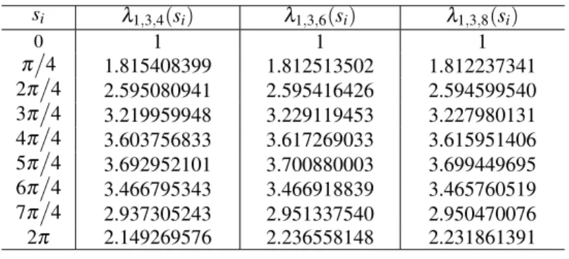
Table 1:Comparison of the approximate solutionsλ1,N,M(s)forN=3 andM=4,6,8.
si λ1,3,4(si) λ1,3,6(si) λ1,3,8(si)
0 1 1 1
Table 2:Comparison of the approximate solutionsλ2,N,M(s)forN=3 andM=4,6,8.
si λ2,3,4(si) λ2,3,6(si) λ2,3,8(si)
0 4 4 4
π/4 3.705079965 3.732993502 3.730369359 2π/4 3.312765003 3.357732448 3.355470705 3π/4 2.950123340 2.982434532 2.980565716 4π/4 2.714155384 2.734770119 2.732536442 5π/4 2.671793724 2.705579966 2.703910773 6π/4 2.859903133 2.913132538 2.910841823 7π/4 3.285280563 3.287920907 3.285146483 2π 3.924655149 3.677999237 3.707601606
Table 3:Comparison of the approximate solutionsλ3,N,M(s)forN=3 andM=4,6,8.
si λ3,3,4(si) λ3,3,6(si) λ3,3,8(si)
0 2 2 2
π/4 1.947930489 1.949879504 1.949081651 2π/4 1.730340565 1.734929919 1.734327739 3π/4 1.302743559 1.302368008 1.302037820 4π/4 0.684100035 0.676520866 0.676111342 5π/4 -0.043182214 -0.043622926 -0.043278513 6π/4 -0.733248164 -0.717268464 -0.717296996 7π/4 -1.176795563 -1.225075999 -1.225287853 2π -1.101074493 -1.562828725 -1.508434184
It is seen from Table 1-3 that the approximate solutions are almost identical. We can write the distance functiondN,Mfrom (25) as
dN,M= √
λ2
1,N,M+λ22,N,M+λ32,N,M=k, k∈. Now, let us calculate the values ofdN,MforN=3 andM=4,6,8. Hence,
d3,4=(0.5e−9)[−(0.236741589992000e19)s2+ (0.180734423860000e19)s3+287950928880522s8
−(0.844546189650672e17)s5+ (0.418460996545252e17)s6−(0.589169688884716e16)s7
+ (0.84e20)−(0.335799929391549e18)s4](1/2)
d3,6=(0.1e−10)[(0.131848677860000e22)s2−(0.191241309980000e22)s3+ (0.21e24)
−(0.159390765639094e19)s7+ (0.317809394084149e19)s8−(0.118264691963043e19)s9
+ (0.192015156647224e18)s10−(0.151904297315817e17)s11+482234023680346s12
+ (0.108855850895550e22)s4−(0.271104120918496e21)s5+ (0.201564518124391e20)s6](1/2)
d3,8=(0.2e−12)[101536780000s−(0.334142178500000e24)s2+ (0.738766435e24)s3+ (0.525e27)
−(0.255765080554550e21)s9+ (0.957793165321548e20)s10−(0.479903869336240e20)s11
+ (0.242465055651551e18)s14−(0.129861616448192e17)s15+ (0.144774173512770e20)s12 −(0.246636805567016e19)s13+295520607607205s16+ (0.127687136841916e23)s7
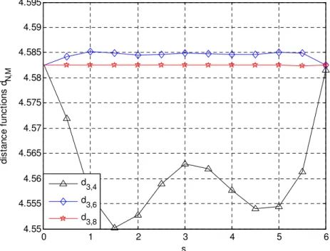
Table 4:Numerical results of distance functionsdN,MforN=3 andM=4,6,8.
si d3,4(si) d3,6(si) d3,8(si) 0 4.582575 4.582576 4.582576
π/4 4.562648 4.585027 4.582442 2π/4 4.550048 4.584816 4.582469 3π/4 4.557248 4.584571 4.582459 4π/4 4.563080 4.584897 4.582465 5π/4 4.558316 4.584602 4.582459 6π/4 4.553611 4.584795 4.582468 7π/4 4.561324 4.584935 4.582444 2π 4.608106 4.579553 4.582891
Now, let us draw the graphics of the distance functionsdN,M for N=3 and M=4,6,8.
0 1 2 3 4 5 6
4.55 4.555 4.56 4.565 4.57 4.575 4.58 4.585 4.59 4.595
s
d
is
ta
n
c
e
f
u
n
c
ti
o
n
s
d N
,M
Figure 1. Comparison of distance functions
d
3,4
d
3,6
d
3,8
It is seen from Table 4 and Figure 1 that accuracy of the solution of system (28) increase when the value ofM is increased. In addition,dN,M is closing a constant value as the value ofM is selected big. This value is breadth of the curve pair of constant breadth. Hence, we can say that the present method is very effective.
M=4,6,8,(i=1,2,3).
e1,3,4(s) =(0.6879998068e−1)s2−(0.3101720095e−1)s3+ (0.358834023138630138e−2)s4
e1,3,6(s) =(0.5414259050e−1)s2−(0.1419290993e−1)s3+ (0.780946093192976150e−3)s5
−(0.328376246375317054e−4)6−(0.22724979443498158924e−2)s4
e1,3,8(s) =(0.5383976860e−1)s2−(0.1474210573e−1)s3−(0.449362456550112302e−5)s7
+ (0.139070836974095252e−6)s8−(0.16320200368388819474e−2)s4
+ (0.51987164532193863786e−3)s5+ (0.17566163126409611616e−4)s6.
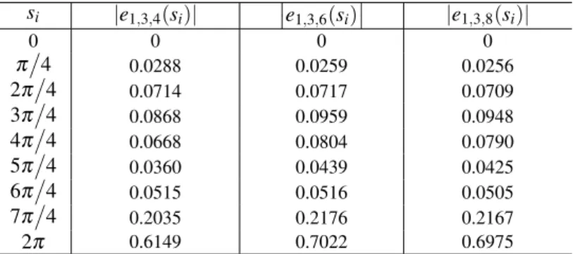
Table 5:Comparison of the estimated absolute error functions|e1,N,M(s)|forN=3 andM=4,6,8.
si |e1,3,4(si)|
e1,3,6(si)
|e1,3,8(si)|
0 0 0 0
π/4 0.0288 0.0259 0.0256
2π/4 0.0714 0.0717 0.0709
3π/4 0.0868 0.0959 0.0948
4π/4 0.0668 0.0804 0.0790
5π/4 0.0360 0.0439 0.0425
6π/4 0.0515 0.0516 0.0505
7π/4 0.2035 0.2176 0.2167
2π 0.6149 0.7022 0.6975
e2,3,4(s) =(0.509072205e−1)s2−(0.2593170193e−1)s3+ (0.329254069115442410e−2)s4
e2,3,6(s) =(0.430535746e−1)s2−(0.5323918129e−1)s3+ (0.20829016919357967950e−1)s4
−(0.300128817280402279e−2)s5+ (0.121540192683128125e−3)s6
e2,3,8(s) =−(0.270211100e−1)s2+ (0.2889273980e−1)s3−(0.702607695411888776e−4)s7
+ (0.221094199053020487e−5)s8−(0.55555395786277287546e−2)s4 −(0.19018036742970799332e−2)s5+ (0.71348969074471050696e−3)s6.
Table 6:Comparison of the estimated absolute error functions|e2,N,M(s)|forN=3 andM=4,6,8.
si |e2,3,4(si)|
e2,3,6(si)
|e2,3,8(si)|
0 0 0 0
π/4 0.0201 0.0078 0.0052
2π/4 0.0452 0.0002 0.0024
3π/4 0.0449 0.0126 0.0144
4π/4 0.0191 0.0015 0.0007
5π/4 0.0023 0.0361 0.0344
6π/4 0.0405 0.0127 0.0105
7π/4 0.2376 0.2349 0.2377
e3,3,4(s) =(0.4e−18)s+ (0.1214120804)s2−(0.5878895125e−1)s3+ (0.694771346566892910e−2)s4
e3,3,6(s) =−(0.20840e−15)s−0.1217448485s2+ (0.5055487825e−1)s3+ (0.453694473233072774e−3)s4
−(0.205140773861414456e−2)s5+ (0.179925190950981802e−3)s6 e3,3,8(s) =−(0.10189678e−14)s+0.1176575974s2−(0.4562781861e−1)s3
−(0.394613814952812954e−4)s7+ (0.262930012001328484e−5)s8−(0.22358445035079499478e−2)s4
+ (0.19778385702964519922e−2)s5+ (0.471203000543214462e−5)s6.
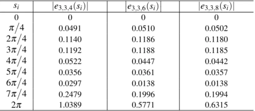
Table 7:Comparison of the estimated absolute error functions|e3,N,M(s)|forN=3 andM=4,6,8.
si |e3,3,4(si)|
e3,3,6(si)
|e3,3,8(si)|
0 0 0 0
π/4 0.0491 0.0510 0.0502
2π/4 0.1140 0.1186 0.1180
3π/4 0.1192 0.1188 0.1185
4π/4 0.0522 0.0447 0.0442
5π/4 0.0356 0.0361 0.0357
6π/4 0.0297 0.0138 0.0138
7π/4 0.2479 0.1996 0.1994
2π 1.0389 0.5771 0.6315
It is seen from Table 5-6-7 that the results are almost identical and close to zero. In addition, we say that the Lucas collocation method is very effective for solving differential equations with variable coefficients. Because, It is very difficult to find the analytical solutions of these differential equations systems.
7 Conclusions
In this study, we have developed a new collocation method based on Lucas polynomials for solving linear differential equation system in normal form with the help of the residual error function. Then, we have given approximate solutions of system of differential equations characterizing curve pair of constant breadth by using Lucas collocation method. We have given an example to demonstrate efficiency and applicability of the present method.
In Figure 1, we have obtained the graphics of the distance function. Also, we have studied the residual error analysis. It is seen from these comparisons that the approximate solutions are very close to absolute solutions when the values ofN
andMare selected big. In addition, Lucas collacation method used for approximate solutions is very effective.
References
[1] L. Euler,De curvis triangularibus, Acta Acad. Petropol., 3-30, (1778), (1780). [2] N. H. Ball,On ovals, American Mathematical Monthly, 37(7): 348-353,1930.
[4] W. Blaschke,Leibziger Berichte, 67 : 290, 1917.
[5] A. P. Mellish,Notes on Differential Geometry, Annals of Mathematics, 32(1): 181-190, 1931. [6] M. Fujiwara,On Space Curves of Constant Breadth, Tohoku Mathematical Journal, 5: 180-184, 1914.
[7] P. C. Hammer,Constant Breadth Curves in the Plane, Procedings of the American Mathematical Society, 6(2): 333-334, 1955. [8] F. Reuleaux,The kinematics of machinery, Trans. by A. B. W. Kennedy, Dover Pub. New York, 1963.
[9] S. Smakal,Curves of Constant Breadth, Czechoslovak Mathematical Journal, 23(1): 86-94, 1973.
[10] ¨O. K¨ose,D¨uzlemde Ovaller ve Sabit Genis¸likli E˘grilerin Bazı ¨Ozellikleri, Do˘ga Bilim Dergisi, Seri B, 8(2): 119-126, 1984. [11] ¨O. K¨ose,On Space Curves of Constant Breadth, Do˘ga Tr. J. Math, 10(1): 11-14, 1986.
[12] A. Ma˘gden, ¨O. K¨ose,On the Curves of Constant Breadth in E4-Space, Tr. J. of Mathematics, 21: 277-284, 1997.
[13] Z. Akdo˘gan, A. Ma˘gden,Some Characterization of Curves of Constant Breadth in En-Space, Turk J Math, 25: 433-444, 2001.
[14] M. Sezer,Differential Equations Characterizing Space Curves of Constant Breadth and a Criterion for These Curves, Turkish J. of Math, 13(2): 70-78, 1989.
[15] M. ¨Onder, H. Kocayi˘git, E. Candan,Differential Equations Characterizing Timelike and Spacelike Curves of Constant Breadth in Minkowski 3-Space E13, J. Korean Math. Soc. 48(4): 849-866, 2011.
[16] H. Kocayi˘git, M. ¨Onder,Space Curves of Constant Breadth in Minkowski 3-Space, Annali di Matematica, 192(5): 805-814, 2013. [17] H. Kocayi˘git, M. C¸ etin,Space Curves of Constant Breadth according to Bishop Frame in Euclidean 3-Space, New Trends in
Mathematical Sciences, 2(3): 199-205, 2014.
[18] M. C¸ etin, M. Sezer, H. Kocayi˘git,Determination of the Curves of Constant Breadth according to Bishop Frame in Euclidean 3-Space, New Trends in Mathematical Sciences (In Press).
[19] M. Sezer, A. Karamete, M. G¨ulsu,Taylor polynomial solutions of systems of linear differential equations with variable coefficients, International Journal of Computer Mathematics, 82(6) : 755-764, 2005.
[20] M. C¸ etin, M. Sezer, C. G¨uler,Lucas Polynomial Approach for System of High-Order Linear Differential Equations and Residual Error Estimation, Mathematical Problems in Engineering, Vol. 2015, 14 Pages, 2015.
[21] A. J. Hanson, H. Ma,Parallel transport approach to curve framing, Indiana University, Techreports-TR425, January 11, 1995. [22] R. L. Bishop,There is More Than One Way to Frame a Curve, American Mathematical Monthly, 82(3): 246-251, 1975.
[23] A. J. Hanson, H. Ma,Quaternion Frame Approach to Streamline Visualization, IEEE Transactions on Visulation and Computer Graphics, 1(2): 164-174, 1995.
[24] F. A. Oliveira,Collocation and residual correction, Numer. Math., 36: 27-31, 1980.
[25] ˙I. C¸ elik,Approximate calculation of eigenvalues with the method of weighted residuals-collocation method, Applied Mathematics and Computation, 160(2): 401-410, 2005.
[26] S. Shahmorad,Numerical solution of the general form linear Fredholm-Volterra integro-differential equations by the Tau method with an error estimation, Applied Mathematics and Computation, 167(2): 1418-1429, 2005.
[27] ˙I. C¸ elik,Collocation method and residual correction using Chebyshev series, Applied Mathematics and Computation, 174(2): 910-920, 2006.
[28] P. Filipponi, A. F. Horadam,Second derivative sequences of Fibonacci and Lucas polynomials, The Fibonacci Quarterly, 31(3) (1993), 194-204.