ISSN 0101-8205 www.scielo.br/cam
Matrix differential equations and inverse
preconditioners
JEAN-PAUL CHEHAB
Laboratoire de Mathématiques Paul Painlevé, UMR 8524
Université de Lille 1, Bât. M2, 59655 Villeneuve d’Ascq cedex, France; and Laboratoire de Mathématiques, UMR 8628
Equipe Analyse Numérique et EDP, Bât. 425, Université Paris XI 91405 Orsay cedex, France
E-mail: [email protected]
Abstract. In this article, we propose to model the inverse of a given matrix as the state of a proper first order matrix differential equation. The inverse can correspond to a finite value of the independent variable or can be reached as a steady state. In both cases we derive corresponding dynamical systems and establish stability and convergence results. The application of a numerical time marching scheme is then proposed to compute an approximation of the inverse. The study of the underlying schemes can be done by using tools of numerical analysis instead of linear algebra techniques only. With our approach, we recover some known schemes but also introduce new ones. We derive in addition a masked dynamical system for computing sparse inverse approximations. Finally we give numerical results that illustrate the validity of our approach.
Mathematical subject classification: 65F10, 65F35, 65L05, 65L12, 65L20, 65N06.
Key words: matrix differential equation, numerical schemes, numerical linear algebra, pre-conditioning.
1 Introduction
The modern methods we have at our disposal for solving linear systems of equa-tions such as the preconditioned versions of GMRES [19] or BI-CGSTAB [21],
are robust and apply to many situations; they are intensively used for the numer-ical solution of large sparse linear systems coming out from PDE discretisation. For this reason the preconditioning is still now a central topic in numerical linear algebra since it is the common universal approach to accelerate the solution of a linear system by an iterative method. Preconditioning a matrix practically leads to improve its spectral properties, by, e.g., concentrating the spectrum of the preconditioned matrix. There is not an efficient general method for building a preconditioner for a given nonsingular matrix : a large number of approaches have been developed depending on the properties of the considered matrix, surveys are presented, e.g., in [4, 19].
Let P be a n ×n regular matrix and b ∈ Rn. The preconditioning of the
numerical solution of the linear system
Pu=b, (1.1)
(with a descent method) consists in solving at each step of the iterative process, an additional linear system
Kv=c, (1.2)
whereKis the preconditioning matrix. Of course, the additional computation carried by the solution of (1.2) is convenient when this system is easy to solve and whenK(respectivelyK−1) resemblesP(resp.P−1).
When the preconditioning of (1.1) is obtained by approachingP, system (1.2) must be easy to solve. In the other case, the approximation ofP−1, which defines the so-called inverse preconditioner, leads to a trivial solution of (1.2).
Inverse preconditioners can be built in many ways: by minimizing an objec-tive functional (the Frobenius norm of the residual, [10]), by incomplete sparse factorization [9], or also by building proper convergent sequences, see [5, 10] in which the authors have presented sequences generated by descent methods such as MINRES or Newton-like schemes. The polynomial preconditioning, which consists in approaching the inverse of a matrix by a proper polynomial, has been developed and implemented for parallel computers, see [19].
also to an equilibrium point, depending on the equation. In such a way, the implementation of any numerical integration can produce an approximation of P−1, say an inverse preconditioner of P. The underlying schemes involve at least one multiplication of two matrices at each iterations so the terms of the sequence of inverse preconditioners become denser even if the matrixPis sparse. However, it is possible to derive a masked dynamical system which preserve a given density pattern making our method suitable for computing sparse inverse preconditioners. From a technical point of view, the advantage of the dynamical system approach is to use the classical tools of numerical analysis of differential equations for studying the processes.
This approach is very flexible since the construction of the numerical scheme is subjected to the choice of the modelling ODE and of a time marching scheme; it allows also to study the schemes by using classical mathematical tools of ODE analysis and of numerical analysis of ODEs [15, 16, 20]. We mention that the use of differential equation modeling for solving systems of equations, including linear algebra problems, was considered in other situations: in [14, 17] for generating flows of matrices that preserve eigenvalues, singular values; in [8] for generating fixed point methods, the solution being defined as a stable steady state; in [13] for computing the square root of a matrix, by integrating a Riccati matrix differential equation (see also R. Bellman’s book [3], chap 10).
2 Inverse at finite time
2.1 Derivation of the equation
Let P(t) andQ(t) be two square matrices, depending on the scalar variablet which belongs to an interval I. We assume that the coefficients of both P and
Qare differentiable functions oft. We have d P(t)Q(t)
dt = d P(t)
dt Q(t)+P(t) d Q(t)
dt , ∀t∈ I.
Assume thatP(t)is regular, i.e. invertible, for alltinIand consider the particular situation Q(t)=P−1(t),
∀t ∈ I. Then we have d P(t)Q(t)
dt =0. So,
d Q(t)
dt = −Q(t) d P(t)
dt Q(t) or, equivalently, d P(t)
dt = −P(t) d Q(t)
dt P(t),
(2.1)
for allt ∈ I. IfP(t)is supposed to be known, thenQ(t)can be computed by integrating the differential matrix equation:
d Q(t)
dt = −Q(x) d P(t)
dt Q(t), t∈ I, Q(0)= P−1(0).
(2.2)
Qis hence the solution of a matrix Riccati differential equation.
Let nowPbe a regularn×nmatrix andI d, then×n identity matrix. Now, the basic idea consists in defining P(t) as a simple path function of regular matrices between P(0) easy to invert (Q(0) = P−1(0)) and P(1) = P. We consider the function
P(t)=(1−t)I d+tP, t∈ [0,1]. (2.3)
Assume that P(t) is invertible for all t in[0,1]. The Matrix Q(t) = P−1(t) satisfies the Cauchy problem
d Q(t)
dt = −Q(t)(P−I d)Q(t) t∈ I, Q(0)= I d,
andP−1
= Q(1); we assume that[0,1] ⊂ ¯I. We have the following result:
Lemma 1. P(t)is regular for all t in[0,1]iff S P(P) ⊂R2\ {(t,0),t ≤ 0} where S P(P)denotes the spectrum of P.
Proof. The eigenvalues of P(t)are the numbers
S(t)=(1−t)+tλ=0, λ∈ S P(P).
Taking the real and the imaginary parts of this expression, we have
φ1(t)=(1−t)+tℜ(λ), φ2(t)=tℑ(λ).
Let us look to necessary and sufficient conditions for havingφ1(t)=φ2(t)=0 for samet. By continuity, it is easy to see thatφ1(t)=0 if and only ifℜ(λ)≤0.
φ2(t)vanishes fort=0 (but P(0)= I d) or forℑ(λ)=0.
In conclusion S(t)vanishes if and only if there existsλ ∈ S P(P)such that
ℜ(λ)≤0 andℑ(λ)=0.
Particularly, Lemma 1 applies whenPis positive definite, such as, e.g., dis-cretization matrices of elliptic operators.
Remark 1. We can consider P(t)=(1−t)P0+tPwithP0a preconditioner of P. Of course, in this case, Lemma 1 applies replacingP by P0−1P. Same considerations can be made with a more general path
P(t)=(1−φ(t))P0+φ (t)P,
with
φ (t): [0,1] → [0,1], φ ∈C1([0,1]), φ′(t) >0,t ∈]0,1[.
2.2 Stability results
2.2.1 Matrix norms
LetM be an×nmatrix. We denote byMany matrix norm ofMand partic-ularly,M2andMFthe 2-norm and the Frobenius norm of M, respectively.
We shall use also the notationv2for the 2 norm of a vector ofRn, there will be no ambiguity in practice.
2.2.2 Hadamard Matrix Product
We denote byR∗Mthe Hadamard product of RandM:
(M∗R)i,j = Ri,jMi,j.
2.2.3 Matrix scalar product
We will use the following scalar product:
≪ R,M ≫ =
n
i,j=1
Ri,jMi,j,
which coincide with the sum of the coefficient of the Hadamard product of R andM. We also use the euclidean scalar product of vector ofRnthat we note by <·,·>.
We begin with the following very simple but useful technical result:
Lemma 2. Let R and S be two n×n matrices. We have the inequalities
(i)
n
i,j=1
|(R2∗R2)i,j| ≤ R4F,
(ii)
n
i,j=1
|(R2∗S)i,j| ≤ R2FSF,
Proof. Assertion (i) follows from a simple application of Cauchy-Schwarz inequality.
Let us prove (ii). We have
|(R2
∗S)i,j| = | n
k=1
Ri,kRk,j
Si,j|,
(using Cauchy Schwarz inequality inRn),
≤
n
k=1 R2i,k
1/2 n
k=1 R2k,j
1/2
|Si,j|.
We now take the sum of these terms fori,j =1,· · ·n. We obtain
n
i,j=1
|(R2∗S)i,j| ≤ n
i,j=1 |Si,j|
n
k=1 Ri,k2
1/2 n
k=1 Rk,2j
1/2 ,
(using Cauchy Schwarz inequality inRn2),
≤
n
i,j=1 Si,j2
1/2
n
i,j=1
( n
k=1 Ri,k2
n
k=1 Rk,2j
1/2
,
≤ R2
FSF.
Assertion (iii) is classical and obtained by applying Cauchy-Schwarz inequality
toSv22= n
i=1
n
j=1 Si,jvj
, forv ∈Rn,v2=1.
At this point, we can establish a stability result:
Proposition 1. Assume that I d−PP−01satisfy the assumptions of Lemma1. We set S(t)=(P−P0)Q(t), where Q(t)solves the equation
d Q(t)
dt = −Q(t)(P−P0)Q(t) t ∈ I, Q(0)=P0−1.
(2.5)
Assume thatS(0)F <1. Then S(t)exists for all t in[0,1]and
S(t)F ≤
1
1− 1
Proof. Multiplying on the left each term of (2.7) byP−P0, we obtain
d S(t)
dt = −S(t) 2
.
We now take the Hadamard product of each term with S(t), and consider the sum of all indicesi,j =1,· · ·,n. We find
1 2
dS(t)2F
dt = −
n
i,j=1
(S(t)2)i,jS(t)i,j,
((ii) of Lemma 2),
≤ S(t)3F. Hence,S(t)2
F ≤ y(t), wherey(t)is the solution of the differential equation
d y(t)
dt =2y(t)3/2 y(0)= S(0)2F
(2.6)
We find
y(t)= 1
1 √
y(0) −t 2 =
1
1
S(0)F −t 2.
SinceS(0)F <1,y(t)remains bounded andy(t)≤ y(1).
Another stability result can be derived when assuming both P andP0 to be symmetric, positive definite (SPD). More precisely we have the next result:
Lemma 3. Assume that bothPandP0are SPD. Then Q(t)= P(t)−1is SPD for all t ∈ [0,1].
Proof. It suffices to prove that P(t)is SPD for all t ∈ [0,1]. The proof is straightforward starting from the definition of P(t):
2.3 Construction of an inverse preconditioner by numerical integration Let us subdivideI = [0,1]intoNsubintervals of the same lengthδ=1/N, the step-length. The application of any (stable) time marching scheme to equation (2.4) generates a sequence Qk,k = 1,· · ·,N, Qk being an approximation of
Q(k/N). In particular, sinceQ(1)=P−1,Q
Nwill be an inverse preconditioner
for the matrixP.
For each time integration scheme, a method for computing a preconditioner is derived. We consider the following cases.
Forward Euler Scheme We consider the sequence
Q0= I d
For k=0,...,N-1
Qk+1=Qk− N1 Qk(P−I d)Qk
(2.7)
We have QN ≃P−1.
Second order Adams Bashforth (AB2) We consider the sequence
Q0=I d
Computation of Q1 by RK2 K0=Q− 21NQ0(P−I d)Q0 Q1=Q0− N1 K0(P−I d)K0 For k=1,...,N-1
Qk+1= Qk− 21N (3Qk(P−I d)Qk−Qk−1(P−I d)Qk−1)
(2.8)
We have QN ≃P−1.
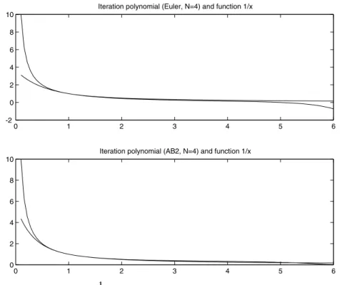
It is easy to see that the above schemes consist in approaching P−1 with a polynomial ofP,PN(P), whose coefficients are matrix independent. The degree
of PN(P) grows exponentially with N. For instance, we have the following
expressions ofPN(P)when it is seen as a one variable function:
Euler’s
N =1 PN(t) = 2−t
N =2 PN(t) = −18(t−3)(t2−4t+7)
N =3 PN(t) = −21871 (t−4)(t2−5t+13)(t4−10t3+42t2−85t+133)
AB2’s
N =1 PN(t) = 134 −154 t+74t2−14t3
N =2 PN(t) = 160194096 −251734096t+208154096 t2−102174096t3+32254096t4
−4096639 t5+ 69 4096t
6
−40963 t7
N =3 PN(t) = 1088391168515661916 −3581936773362797056 t+1484035553120932352 t2
−113942038311088391168t3+2404253335
362797056 t4−391144243120932352t5 +13528681571088391168t6− 46022507
120932352t7+134369281251827 t8 −108839116819757677 t9+ 1008073
362797056t 10
−12093235239389 t11 +108839116830455 t12− 595
362797056t 13
+1209323527 t14 −10883911681 t15
These polynomials are approximations of the functiont → 1t, as illustrated in Figure 1.
0 1 2 3 4 5 6 -2
0 2 4 6 8 10
Iteration polynomial (Euler, N=4) and function 1/x
0 1 2 3 4 5 6
0 2 4 6 8 10
Iteration polynomial (AB2, N=4) and function 1/x
Figure 1 – The function 1x and the iteration polynomials a) Euler, N = 4, b) AB2, N =4.
orthogonal polynomial[1], see[2,4]for a review. However, the point of view here is different and the underlying polynomial are also different.
At this point we give a convergence result for the Euler method (scheme (2.9)). More precisely, we give a consistency error bound. We have the
Theorem 1. Assume that P −P0 is regular and satisfies the hypothesis of Lemma1. Let QN, be the approximation of Q(1)obtained by replacing
d Q(t)
dt
k N
by Q
k N
−Qk−N1 1
N
.
Assume that the solution of(2.7)isC2. Then Q(1)−QN2≤
1
2N(P−P0)
−1 2
1
1− 1
Proof. We have
Q(1)−Q(0) = 1
0
d Q(t)
dt dt
=
N
k=1
k
N k−1
N
d Q(t)
dt dt
Letk be fixed and lett ∈]k−N1, k
N[. There existst0∈]k−N1,t[such that d Q(t)
dt = d Q
dt
k−1 N
+t−k−N1d2Q dt2 (t0), (Q(t)being solution of (2.7))
= −Qk−N1(P−P0)Qk−N1
+2
t− k−N1
Q(t0)(P−P0)Q(t0)(P−P0)Q(t0),
= −Q
k−1 N
(P−P0)Q
k−1 N
+2t− k−N1(P−P0)−1((P
−P0)Q(t0))3. Hence,
k
N k−1
N
d Q(t)
dt dt− 1 N
−Q
k−1 N
(P−P0)Q
k−1 N
2
≤ 1
N2(P−P0)
−1 2 sup
t∈[0,1]
(P−P0)Q(t)32. Therefore, we have the estimate:
Q(1)−QN2 ≤
N
k=1 1
N2(P−P0)
−1 22 sup
t∈[0,1]
(P−P0)Q(t)3,
≤ N1(P−P0)−12 sup
t∈[0,1]
(P−P0)Q(t)3F),
≤ N1(P−P0)−12y(1). where y(t)is solution of (2.8), and
y(1)= 1
1− 1
I d−PP−01F
The Euler scheme preserves the symmetry. In particular we can prove that for P,P0,P−P0SPD, and forN large enough, the matricesQkgenerated by (2.9)
are SPD fork =0,· · · ,N.
3 Inverse matrix as steady state
3.1 The equations
Another way to reachP−1is to consider differential equations for which one of the steady states is Q=P−1. We consider the two following equations:
d Q(t)
dt =Q(t) (I d−PQ(t)) , Q(0)=Q0,
(3.11)
which is a Riccati matrix differential equation and its linearized version
d Q(t)
dt = I d−PQ(t),t ≥0 Q(0)=Q0.
(3.12)
In both equationsP−1is a steady state.
Remark 3. We can also proceed as in Section 2: we consider equation(2.4) with the path function P(t):
P(t)=(1−e−t)P+e−tP0.
It is easy to see that P(t) is invertible for allt ≥ 0 iffPP−01 satisfies the as-sumptions of Lemma 1, see also Remark 1. The differential equation satisfied by Q(t)is then
d Q(t)
dt =e−
tQ(t)(P
−P0)Q(t),t≥0,
Q(0)=Q0.
We now give sufficient conditions for obtaining the convergence lim
t→+∞Q(t)=
P−1. We propose two approaches. The first one consists in deriving bounds of the Frobenius norm of the solution, assuming that the initial data is close enough to the steady state. The second one concentrates on the symmetric definite positive case.
Proposition 2. Let Q(t) be the solution of the matrix differential equation
(3.11). Assume thatI d−PQ0F <1. Then lim
t→∞Q(t)=P −1.
Proof. The matrix R(t)=I d−PQ(t)satisfies the equation d R(t)
dt = −R(t)+R 2(t).
Then, taking the Hadamard product of each terms with R(t)and taking the sum of all the coefficients, we obtain
1 2
dR(t)2F
dt + R(t) 2
F = −
i,j
(R2∗R)i,j.
By the first assertion of Lemma 2 (withS =R), we have
1 2
dR(t)2F
dt + R(t) 2
F ≤ R(t)
3
F.
From the previous inequality, we infer thatR(t)2F is bounded from below by the solution of the scalar differential equation
d y(t)
dt = −2y(t)(1− √
y(t))
y(0)= I d−PQ02
F
We have
y(t)= 1
1+
1 √
y(0)−1
et
2,
hence the result.
This last results insures the existence of solution and the convergence toP−1for initial conditions closed enough to the steady state; however no other properties ofPor ofQ0are required. We now give an existence and a convergence result in the symmetric positive definite case. We have the
Proposition 3. Assume thatPand Q(0)are SPD matrices. Then Q(t)is SPD for all t ≥0and lim
Proof. IfQ(t)is regular for allt, thenU(t)= Q(t)−1satisfies the differential equation
dU(t)
dt = −U(t)+P, x ≥0, U(0)=Q−1(0).
We prove the proposition by studyingU(t). We have
U(t)=(1−e−t)P+e−tU0,
from which we infer thatU(t)is SPD for allt ≥ 0. Indeed,U(t)is symmetric as sum of symmetric matrices, and for everyw∈Rn, we have
U(t)w, w =(1−e−t)Pw, w +e−tP0w, w>0,
since bothPandP0are assumed to be positive definite. Furthermore, we have immediately lim
t→∞U(t)=P. ThereforeU(t)is SPD for allt ≥0. In conclusion
Q(t)exists and is SPD for allt ≥0 and lim
x→∞Q(t)=P −1.
Proposition 4. Let Q(t)be the solution of(3.12). AssumePis positive definite. Then lim
x→∞Q(t) = P −1
. Moreover ifPand Q0 are SPD and commute withP, thenQ(t)is also SPD for all t≥0.
Proof. As usual, we introduce the residual matrix R(t)=I d−PQ(t)which here satisfies the equation
d R(t)
dt = −PR(t), whose solution is
R(t)=e−tPR(0). Hence, ifPis positive definite, lim
x→∞R(t)=0.
From the expression ofR(t)we infer
Q(t)=(I d−e−tP)P−1+e−tPQ0.
Let us now establish the convergence in the Frobenius norm. IfPis positive definite, there exists a strictly positive real numberαsuch that
α n
i=1
u2i ≤ Pu,u = n
i=1
n
k=1 Pi,kuk
uk,∀u ∈Rn, u =(u1,· · ·,un)t,
the numberαpossibly depending onn.
Taking the Hadamard product of each term of the differential equation and summing on all indicesi, j, we get
1 2
dR2F dt +
n
i,j=1
n
k=1
Pi,kRk,j
Ri,j =0.
Therefore,
1 2
dR2F
dt +αR 2
F ≤0.
By integration of each side of the last inequality, we obtain
R(t)F ≤e−αtR(0)F.
3.2 Construction of preconditioners by numerical integration
We introduce the discrete residual Rk = I d−PQk. The numerical integration
of equation (3.11) by forward Euler’s method generates the sequence Rkwhich
satisfies the recurrence relation:
Rk+1=(1−tk)Rk+tkRk2.
We remark that fortk =1, the convergence is quadratic wheneverR0<1,
where . is any matrix norm. We recover in this case the Newton method derived from the equation in one variable 1t −r =0, see [10].
Let us study the general case.
Theorem 2. We have the following results: (i) k =t . Assume that
ρ(R0) <1 and t < 2 1−ρ(R0).
Then lim
k→∞Qk =P −1
(ii) Assume thatR0F <1and that
0< tk <
2 1+ RkF∀
k.
Then, lim
k→∞RkF = 0. Moreover the convergence is quadratic for
tk =1.
(iii) Assume that Pand Q0 are symmetric, then Qk is also symmetric for all
k ≥0.
Proof. From the relation
Rk+1=Rk((1−t)I d+t Rk) ,
we deduce that the convergence is guaranteed ifρ((1−t)I d+t Rk) < 1,
say if
ρ(R0) <1 and 0< t < 2 1−ρ(R0).
The first condition is verified, e.g., when Q0 = γPT with 0 < γ < 2 ρ(PPT).
Notice that ifPis positive definite, we can takeQ0=γI dwith 0< γ < 2 ρ(P), Hence the assertion (i).
Letkbe fixed. We have
Rk+1∗Rk+1=(1−tk)2Rk∗Rk+2tk(1−tk)Rk∗Rk2.+(tk)2Rk2∗R
2
k.
Taking the sum of all the indices, we obtain
Rk+12F = (1−tk)2Rk2F
+2tk(1−tk) n
i,j=1
n
m=1
(Rk)i,m(Rk)m,j
(Rk)i,j
+(tk)2 n
i,j=1
n
m=1
(Rk)i,m(Rk)m,j 2
,
(applying Lemma 2)
≤ (1−tk)2Rk2F+2tk|1−tk|Rk3F+(tk)2Rk4F,
Therefore, if Mk = |1−tk| +tkRkF < 1, say ifRkF < 1 and 0 < tk < 1 2
+ RkF, thenRk+1F < MkRkF with Mk <1. The contraction
holds in particular when 0< tk ≤1 and it is easy to prove by induction that if
R0F <1 thenRk+1F < MRkF, withM <1. The convergence follows.
The particular casetk =1 gives directly the estimate
RkF ≤ R02
k
F.
The convergence in Frobenius norm is then quadratic in this case ifR0F <1.
The point (ii) is proved.
Finally, ifQ0andPare SPD, then using the relation Qk+1=(1+tk)Qk− tkQkPQk, we show easily by induction that Qk is symmetric for allk ≥ 0.
This completes the proof.
Let us now consider the implementation of the Euler scheme to (3.12). The following sequence of matrices is generated:
Q0given For k=0,...
Qk+1=Qk+tk(I d−PQk)
(3.13)
We have the
Theorem 3. AssumePis positive definite and, for simplicity, thatkt =t .
Then
(i) If 0 < t < 2
ρ(P),∀k ≥ 0. Then, Qk, the sequence generated by the
scheme(3.13)converges toP−1.
(ii) Assume in addition that P is symmetric and Q0 is SPD. Assume that Q0 andP commute. Then Qk is symmetric for all k ≥ 0. Moreover if α0−tMI d1−t P Q02
−M >0then Qkis SPD for all k ≥0, where we have set M = I d−t P2,
α0= min
x∈Rn,x
2=1
Proof. Assume first thattk =t. Using the same notations, we have,
Rk+1=(I d−tP)Rk.
Thus, Rk →0 if and only if 0< t < ρ(2P).
Let us now study the convergence in the Frobenius norm. SincePis positive definite, we can define
0< α= min
u∈Rn,u
2=1
Pu,u u,u . We have
Rk+1∗Rk+1=(I d−tP)Rk∗(I d−tP)Rk.
Hence, taking the sum of all indices, we obtain after simplifications
Rk+12F +2t
i,j n
m=1
Pi,mRm,jRi,j = Rk2F+(t)
2
i,j n
m=1
Pi,mRm,j 2
.
Therefore
Rk+12F+2αtRk2F ≤ Rk2F+(t)
2
P2FRk2F.
Finally
Rk+12F ≤
1−2αt+(t)2P2F
Rk2F,
which gives the (sufficient) stability condition
0< t < 2α
P2F.
Now, one can show by induction that if Q0 and P commute, then Qk and P
commute also for allk ≥0. Then, proceeding also by induction, it can be shown that Qk is symmetric for allk ≥ 0. Notice that the conditionPQ0 = Q0Pis
simply verified, e.g., with the choice Q0=I d. Now we set
αk = min
x∈Rn,x
2=1
Qkx,x
x,x ,∀k ≥0. Letx ∈Rn,x2=1. We have
Qk+1x,x = Qkx,x −tRkx,x,
ButRk ≤ I d−tP2k R02=MkR02. Thus
αk+1≥αk−t MkR02, and therefore
αk ≥α0−t
M(1−Mk)
R02
1−M ≥α0−t
MR02 1−M .
This completes the proof.
By analogy between Euler’s method and Richardson’s iterations, it is natural to computetk such as minimizingRk+1F. We have
Rk+1∗Rk+1=(I d−tkP)Rk∗(I d−tkP)Rk.
Taking the sum on all indices, we obtain, after the usual simplifications
Rk+12F = Rk2F+(tk)2 n
i,j=1
((PRk)∗(PRk))i,j−2tk n
i,j=1
((PRk)∗Rk)i,j.
It follows thatRk+1Fis minimized for
xk = n
i,j=1
((PRk)∗Rk)i,j
PRk2F
= ≪PRk,Rk ≫ ≪PRk,PRk ≫
,
and we recover the iterations proposed in [10], see also Section 4.
3.3 Steepest descent-like Schemes
For example, in [8] it was defined a method for computing iteratively fixed points with larger descent parameter starting from a specific numerical time scheme. It consists in integrating the differential equation
dU
dt = F(U), U(0)=U0,
(3.14)
by the two steps scheme
K1=F(Uk),
K2=F(Uk
+t K1),
Uk+1=Uk+t(αK1+(1−α)K2) .
(3.15)
Here α is a parameter to be fixed. This scheme allows a larger stability as compared to the Forward Euler scheme. More precisely, whenF(U)=b−PU.
Lemma 4. Assume thatPis positive definite, then the scheme is convergent iff
α < 7
8 and t<
1 (1−α)ρ(P).
Of course, one can define iterativelyαandtsuch as minimizing the euclidean norm of the residual, exactly as in the steepest descent method. The residual equation is
rk+1=I −tk P+(1−αk)(tk)2P2
rk. (3.16)
Hence
rk+12 = rk2−2tkPrk,rk +(tk)2Prk2
+2(1−αk)(tk)2P2rk,rk −2(1−αk)(tk)3P2rk,Prk
+(1−αk)2(tk)4P2rk,P2rk.
We set for convenience
a= rk
2, b= Prk,rk
, c= Prk
2,
d = P2rk,rk
, e= P2rk,Prk
, f = P2rk,P2rk
.
rk+1
is minimized for the following definition of the parameters:
tk =
f b−ed
f c−e2, αk =(f c−e 2
4 Sparse inverse preconditioners
The iterative processes generated by numerical integration of the differential equations require at least a product of two matrices at each iteration. Hence, at each iteration, the inverse preconditioner matrix becomes denser, even if the initial data and the matrix to invert are sparse.
We propose here a simple way to derive a dropping strategy from the numerical integration of a matrix differential equation. The notations are the same as in the previous sections. Consider the equation
d Q
dt =I d−PQ, Q(0)= Q0.
(4.17)
HerePis a positive definite matrix so lim
x→∞Q(x)= P
−1, a shown in section 2.
4.1 Derivation of the equations
Now, letF be an×n matrix with coefficients 0 or 1. The Hadamard product F ∗Preturns a matrix whose coefficients are those of Pwhich have the same indices as the non null coefficients ofF, soF is a filter matrix which selects a sparsity pattern. More precisely, we have
(F ∗P)i,j =
Pi,j ifFi,j =1,
0 else.
We assume thatFi,i =1,i =1,· · ·n, soF ∗I d = I d, where I dis then×n
identity matrix.
At this point, we consider the Hadamard product of each term of (4.17) with F. We obtain the system
dF∗Q
dt = I d−F ∗(PQ), F ∗Q(0)=F ∗Q0.
(4.18)
For deriving an autonomous equation with a sparse matrix S as unknown, we approachF∗(PQ)byF ∗(PFQ)and we obtain the new system
d S
dt =I d−F ∗(PS), F ∗S(0)=F ∗Q0.
The matrix S(t)is sparse for allt. Indeed, we have the
Lemma 5. The matrix equation(4.19)has a unique solution S(t)∈C1(
]0,+∞[
and
F ∗S(t)=S(t),∀t ≥0.
Proof. The existence and the uniqueness of S(t)is established by using stan-dard arguments.
We have
S(t)=S(0)+ t
0
(I d−F ∗(PS))ds
Hence, sinceF ∗S(0)=S(0), we can write
F∗S(t) = S(0)+ t
0
F∗(I d−F∗(PS)ds
= S(0)+ t
0
(I d−F ∗(PS)ds.
We now will show thatS(t)is an approximation ofQ(t).
4.2 A priori estimates We have the following result:
Theorem 4.
S−Q2F ≤ 2×(1−F)∗P−12Fe−tP−I d2FI d−PQ02F + 1
2α(1−F)∗P
−1
2FI d−PQ0
2
F t
0
e−α(t−s)e−sP−I d2Fds, where 1 is the neutral element of the Hadamard product, (1i,j = 1,i, j =
1,· · ·n).
Proof. Taking the difference of the equations (4.19) and (4.18), we get
d S−F ∗Q
The difference between (4.18) and (4.17) gives
dF ∗Q−Q
dt =(1−F)∗PQ. (4.21)
From (4.20), we infer
1 2
dS−F ∗Q2
F
dt = − ≪F∗(P(S−F∗Q)),S−F ∗Q≫ + ≪F∗(P(F∗Q−Q)),S−F∗Q ≫.
(4.22)
Now, since
≪F ∗(P(S−F ∗Q)),S−F ∗Q≫ = ≪P(S−F ∗Q)),S−F∗Q≫,
we can write
1 2
dS−F∗Q2
F
dt + ≪P(S−F ∗Q)),S−F∗Q≫ = + ≪P(F ∗Q−Q),S−F ∗Q≫.
(4.23)
We letα = min
Q∈Mn(R)
≪PQ,Q≫
≪ Q,Q≫ and we deduce from the previous equation
1 2
dS−F ∗Q2
F
dt +αS−F ∗Q 2
F
≤ ≪P(F∗Q−Q),S−F ∗Q≫, (applying Young’s inequality),
≤ η2S−F∗Q2F + 1
2ηF∗Q−Q
2
F.
(4.24)
Here η is a strictly positive real number which will be chosen later on. We now must derive estimates for F ∗Q−QF. From the direct integration of
(4.17), we get
PQ =I d−e−tP(I d−PQ0) . Therefore,
dF∗Q−Q
dt =(1−F)∗
so
(F ∗Q−Q)(t) = (F ∗Q−Q)(0)
+
t
0
(1−F)∗I d−e−tP(I d−PQ0)ds, (4.25)
=
t
0
(1−F)∗e−sP(I d−PQ0)ds, (4.26)
= (1−F)∗ t
0
e−sP(I d−PQ0)ds, (4.27)
= (1−F)∗P−1e−tP−I d(I d−PQ0). (4.28) We then can write
(F∗Q−Q)(t)F ≤ (1−F)∗P−1Fe−tP−I dFI d−PQ0F.
Substituting this last inequality in (4.24), we get
1 2
dS−F ∗Q2
F
dt +αS−F ∗Q 2
F ≤ η
2S−F ∗Q 2
F
+ 1
2η(1−F)∗P
−1 2Fe−
tP
−I d2FI d−PQ02F Now we chooseη=αand we integrate this inequality:
(S−F ∗Q)(t)2F ≤ (S−F ∗Q)(0)2Fe−αt + 1
2α(1−F)∗P
−1
2FI d−PQ0
2
F t
0
e−α(t−s)e−sP−I d2Fds. Finally, summing this last estimate with(F∗Q−Q)(t)2F we obtain
S−Q2F ≤ 2(S−F∗Q
2
F + F∗Q−Q
2
F)
≤ 2×(1−F)∗P−12Fe−tP−I d2FI d−PQ0
2
F
+ 1
2α(1−F)∗P
−1
2FI d−PQ0
2
F t
0
e−α(t−s)e−sP−I d2Fds
5 Numerical illustrations
5.1 Inverse matrix approximation
Consider the problem
−u+a(x,y)∂u
∂x +b(x,y)
∂u
∂y = f in=]0,1[
2 (5.29)
u=0 on∂ (5.30)
We discretize this problem by second order finite differences on an×ngrid and we define Pas the underlying matrix. The numerical results we present were obtained by using Matlab 6 on a cluster of Bi-processor 800 (Pentium III) at Université Paris XI, Orsay, France.
5.1.1 Integration of finite time inverse matrix differential equation
We first consider the problem with
a(x,y)=30ey2−x2, b(x,y)=50 sin(72x(1−x)y)∗sin(3πy), n =30
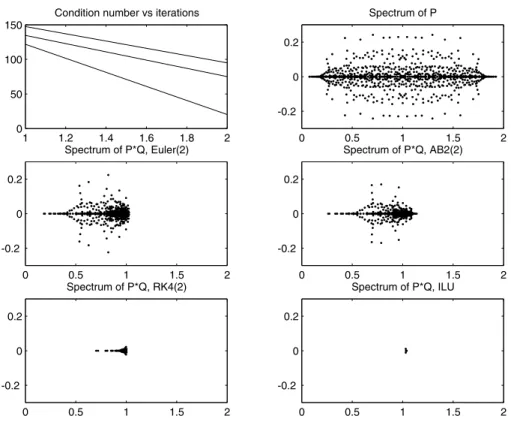
(the matrix is of size 900 ×900) and a Chebyshev Mesh in both directions. In Figure 2 we have compared the preconditioners obtained with 2 iterations of Euler (Euler(2)), of Adams-Bashforth (AB(2)), of Fourth order Runge Kutta (RK4(2)). We observe that the more accurate is the integration method, the more concentrated is the spectrum of the preconditioned matrix.
5.1.2 Sparse inverse preconditioner case
We consider here the sparse approximation of the inverse of the finite differences discretization matrix of the operator
−+500∂x +20∂y
on the domain ]0,1[2 with homogeneous Dirichlet boundary conditions, on a regular grid. Here the sparsity pattern is defined by the n2×n2 symmetric mask-matrixF as follows
1 1.2 1.4 1.6 1.8 2 0
50 100 150
Condition number vs iterations
0 0.5 1 1.5 2 -0.2
0 0.2
Spectrum of P
0 0.5 1 1.5 2 -0.2
0 0.2
Spectrum of P*Q, Euler(2)
0 0.5 1 1.5 2 -0.2
0 0.2
Spectrum of P*Q, AB2(2)
0 0.5 1 1.5 2 -0.2
0 0.2
Spectrum of P*Q, RK4(2)
0 0.5 1 1.5 2 -0.2
0 0.2
Spectrum of P*Q, ILU
Figure 2 – Spectrum ofP,Euler(2)P,A B2(2)P,R K4(2)PandI LUP.
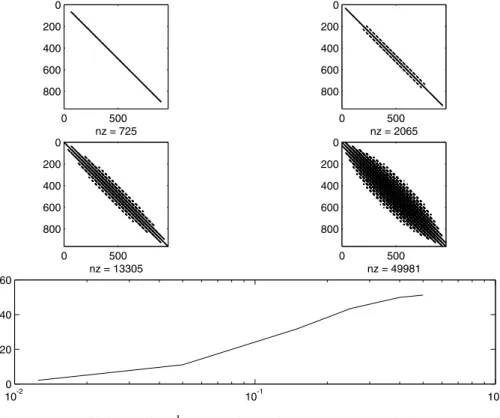
In Figure 3 we have represented approximations of the inverse matrix that are obtained by a tresholding of the coefficient at the levelǫ, for different values of ǫ. This shows that a sparse approximation can be considered in this case.
0 500 0
200
400
600
800
nz = 725
0 500 0
200
400
600
800
nz = 2065
0 500 0
200
400
600
800
nz = 13305
0 500 0
200
400
600
800
nz = 49981
10-2 10-1 100
0 20 40 60
Figure 3 – Coefficients ofP−1greater (in modulus) thanǫ = 0.5 (fig. (a)), ǫ = 0.4 (fig. (b)),ǫ=0.25 (fig. (c)),ǫ=0.15 (fig. (d)), norm of the error for the filtered inverse matrix vsǫ, (e).
5.2 Preconditioned descent methods
The reduction of the condition number as well as the concentration of the spec-trum of the preconditioned matrix allows faster convergence of descent methods. As an illustration, we apply the explicit preconditioner computed above to the numerical solution of the convection diffusion problem. To this end, we use the preconditioned BiCgstab method [21].
The discretization matrix is the same as above. The discrete problem to solve reads
Px =b
equiv-0 5 10 15 20 25 30 35 40 100
102 104 106
0 5 10 15 20 25 30 35 40
100 105 1010 1015
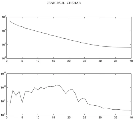
Figure 4 – Computation of sparse inverse preconditioner: Residual vs iterations (above) and condition number vs iterations (below).
alent problem
diag(P)−1Px =diag(P)−1b. The exact solutionxeis a random vector andb=Pxe.
In Figure 6 we have represented the residual (respectively the error) versus the iteration when using Bicgstab and various preconditioned versions; the explicit preconditioners Qwere here generated by, in the one hand, with two iterations of Euler, of AB2 and of RK4, and, in the other hand, with an ILU factorization with ǫ = 10−2as tolerance. The Euler and the AB2 preconditioners improve the convergence of the unpreconditioned method, with respective rates 2 and 3. The RK4 preconditioner is comparable to the ILU one.
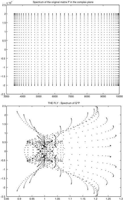
3000 4000 5000 6000 7000 8000 9000 10000 -2.5
-2 -1.5 -1 -0.5 0 0.5 1 1.5 2 2.5x 10
4 Spectrum of the original matrix P in the complex plane
0.85 0.9 0.95 1 1.05 1.1 1.15 1.2 1.25 1.3 -2.5
-2 -1.5 -1 -0.5 0 0.5 1 1.5 2 2.5
THE FLY : Spectrum of Q*P
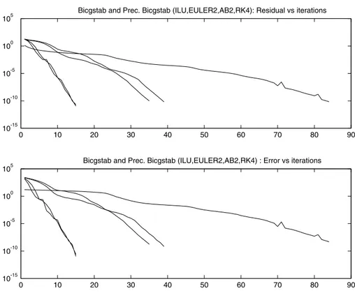
0 10 20 30 40 50 60 70 80 90 10-15
10-10 10-5 100 105
Bicgstab and Prec. Bicgstab (ILU,EULER2,AB2,RK4): Residual vs iterations
0 10 20 30 40 50 60 70 80 90
10-15 10-10 10-5 100 105
Bicgstab and Prec. Bicgstab (ILU,EULER2,AB2,RK4) : Error vs iterations
Figure 6 – Comparison of the preconditioners : Euler(2), AB(2), RK4(2) and ILU, Size of the system : 961×961, a) Residual vs iterations, b) error vs iterations.
6 Concluding remarks
The approach we have developed here is simple, rather general and seems to apply to a large class of matrices. The advantage of this technique is to study the underlying approximations with simple analysis tools; we recover in addi-tion particular sequences of inverse precondiaddi-tioners ([4, 10, 9]) and introduce new ones. The iterative schemes we introduced in this article are all based on approximation of the inverse by a proper polynomial: they can be considered as polynomial preconditioners in spite they are not automatically related to the ones proposed (e.g.) by [1], the point of view being here different. This suggests as a feature to analyze them by using an approach coming from the approximation theory.
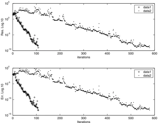
effi-0 100 200 300 400 500 600 10-10
10-5 100 105
iterations
Res. Log.10
data1 data2
0 100 200 300 400 500 600
10-15 10-10 10-5 100
Iterations
Err. Log.10
data1 data2
Figure 7 – Sparse inverse preconditionning for convection-diffusion problem. a) Residual vs iterations; b) Error vs iterations.
cients sparse inverse preconditioners for a fixed sparsity pattern. A natural next feature would be to develop dropping strategies for improving the method.
We have applied here a dynamical modeling approach to the construction of inverse preconditioners. A similar approach can be developed for the solution of linear as well as non linear systems of equations, deriving numerical schemes from special dynamical systems.
The examples we give are coming out from PDE’s discretization and are rather academic, but is it a first step to be considered before developing and applying the schemes to large scales problems.
REFERENCES
[1] Ashby, Manteuffel and Otto, A comparison of adaptive Chebyshev and least squares poly-nomial preconditioning for Hermitian positive definite linear systems, SIAM J. Sci. Stat. Comput.,13(1) (1992), 1–29.
[2] O. Axelsson,Iterative solution methods. Cambridge University Press, Cambridge, 1994. xiv+654 pp.
[3] R.E. Bellman,Introduction to Matrix Analysis, Mcgraw-Hill (New York), 1970 – 2nd ed. [4] M. Benzi, Preconditioning techniques for large linear systems: a survey. J. Comput. Phys.,
182(2) (2002), 418–477.
[5] C. Brezinski,Projection Methods for Systems of Equations, North-Holland, 1997.
[6] C. Brezinski, Dynamical systems and sequence transformation, J. Phys. A: Math. Gen.,34
(2001), 10659–10669.
[7] C. Brezinski, Difference and differential equations and convergence acceleration algorithms. SIDE III-symmetries and integrability of difference equations (Sabaudia, 1998), 53–63, CRM Proc. Lecture Notes, 25, Amer. Math. Soc., Providence, RI, 2000.
[8] C. Brezinski and J.-P. Chehab, Nonlinear hybrid procedures and fixed point iterations, Numer. Func. Anal. Opt.,19(5-6) (1998), 415–487.
[9] G. Castro, J. Laminie, M. Sarrazin and A. Seghier, Factorized Sparse Inverse Preconditioner using Generalized Reflection Coefficients, Prépublication d’Orsay numéro 28 (10/7/1997). [10] E. Chow and Y. Saad, Approximate Inverse Preconditioning for Sparse-Sparse Iterations,
SIAM Journal of Scientific Computing,19(1998), 995–1023.
[11] Eisenstat, Ortega and Vaughan, Efficient polynomial preconditioning for the conjugate gardient method, SIAM J. Sci Stat. Comp.,11(5) (1990), 859–872.
[12] A. Cuyt and L. Wuytack,Nonlinear Methods in Numerical Analysis, North-Holland, Ams-terdam, 1987.
[13] F. Dubois and A. Saidi, Unconditionally stable scheme for Riccati equation, ESAIM Proc,
8(2000), 39–52.
[14] U. Helmke and J.B. Moore,Optimization and Dynamical Systems, Comm. Control Eng. Series, Springer, London, 1994.
[15] M.W. Hirsch and S. Smale,Differential Equations, Dynamical Systems and Linear Algebra, Academic Press, London, 1974.
[16] J.H. Hubbard and B.H. West,Differential equations. A dynamical Systems Approach. Part I: Ordinary Differential Equations, Springer Verlag, New-York, 1991.
[18] Y. Saad, Practical implementation of polynomial preconditioning for Conjugate Gradient, SIAM J. Sci. Stat. Comp.,6(1985), 865–881.
[19] Y. Saad,Iterative Methods for Sparse Linear Systems, SIAM, 1996.
[20] A.M. Stuart, Numerical analysis of dynamical systems, inActa Numerica, 1994, Cambridge University Press, Cambridge, 1994, pp. 467–572.